Another View of Complex Intuitionistic Fuzzy Soft Sets Based on Prioritized Aggregation Operators and Their Applications to Multiattribute Decision Making

Abstract

In a conventional interpretation of decision-making based on ambiguity, a decision-maker must prefer the best possible opportunity including various feasible possibilities. However, the dilemma of picking the best possible alternative has continued to be a substantial task to resolve. In this manuscript, we improve the existing complex intuitionistic fuzzy soft set (CIFSS), which includes the grade of truth and falsity with the rule that the sum of the real and imaginary parts of both grades is confined to [0, 1]. CIFS is a valuable procedure to determine the authenticity and consistency of the elaborated approaches. The fundamental laws and their related examples are also determined. Moreover, by using these laws, we investigated the complex intuitionistic fuzzy soft prioritized weighted averaging operator (CIFSPWAO), the complex intuitionistic fuzzy soft prioritized ordered weighted averaging operator (CIFSPOWAO), the complex intuitionistic fuzzy soft prioritized weighted geometric operator (CIFSPWGO), complex intuitionistic fuzzy soft prioritized ordered weighted geometric operator (CIFSPOWGO), and their related properties are also developed. Based on the developed operators, the multiattribute decision-making (MADM) tool is developed by using the explored operators based on CIFSS. Some numerical examples are also illustrated by using the investigated operators to determine the feasibility and consistency of the developed approaches. Finally, the comparative analysis and their geometrical manifestations are also determined to enhance the excellence of the performed explorations.

1. Introduction

MADM is a mutual procedure in individuals’ everyday natural life and industry organization. In the exploration of MADM procedures, developing and controlling evaluation material is a requirement for achieving the best explanation. Since Zadeh [1] initially suggested the idea of fuzzy set (FS) to illustrate the ambiguity of an object, various conventional expansions of FSs have been offered to adapt to unique decision-making situations, such as the idea of soft set (SS), which was elaborated by Molodtsov [2]. Mahmood [3] developed the notion of bipolar soft set and discussed its application in decision making problems. Between these expansions of FSs, researchers have also sought effective implementations for exhibiting ambiguity and vagueness, which describe every single component with a truth degree belonging to [0, 1]. In the last 30 years, numerous researchers have conducted in-depth investigations and explorations in FS theory, and in consequence a huge number of discoveries have been accomplished within the field of FS, comprising assessment and ranking procedures, aggregation operators, hybrid operators, similarity measures and allowances of traditional MADM approaches, etc. However, there are various concerns that when an individual faced this kind of situation, which includes the grade of truth and falsity, then the FS is not proficient to operate within it. For this purpose, the theory of intuitionistic FS (IFS) was elaborated by Atanassov [4] as a generalization of FS that includes the grade of truth and falsity with the rule that $0\le {\mu }_{{\tilde{\Xi }}_{IF}}+{\eta }_{{\tilde{\Xi }}_{IF}}\le 1$. IFS is an extensive validation procedure used to determine the dependability and consistency of the created approaches. Since its development, this theory has received extensive attention from distinguished scholars and several individuals have utilized it in many directions [5,6,7,8,9,10].

From the above prevailing examinations, it is noted that they are extensively manipulated but that previous researchers have neglected to carry out the time-periodic problems and two-dimensional knowledge mutually in a specific set. In light of this, Ramot et al. [11] suggested the concept of complex FS (CFS) to illustrate the ambiguity of an object discussed above. CFS theory is exhibited by a complex-valued truth function with a codomain unit disc in the complex plane. Since its development, this theory has received extensive attention from distinguished scholars and several individuals have utilized it in many directions, like distance measures and cross-entropy [12], logic [13,14] and neurofuzzy architecture [15]. Keeping in view the effectiveness and importance of CFS theory in the last 15 years, numerous researchers have undertaken in-depth investigation and exploration of CFSs and a huge number of solutions making use of the CFSs have been studied, comprising assessment and ranking procedures, aggregation operators, hybrid operators, similarity measures and allowances of traditional MADM approaches, etc. However, there are various concerns that when an individual is faced with this kind of situation, which includes the grade of truth and falsity in the form of complex-valued, then the CFS is not proficient to operate with it. For this reason, Alkouri and Salleh [16] generalized the notion of CFSs to Complex IFSs (CIFSs) by familiarizing falsity degrees into the assessment. In CIFS theory, complex values of truth and falsity are measured in polar structure. The amplitude terms related with agreeing (disagreeing) values depict the strength of being appropriate (not-being appropriate) for the aspect in the set and the phase terms require extra knowledge, which is correlated with periodicity. These phase terms discriminate the CIFS and IFS theories. IFS nature cannot carry extra one-dimensional problems, which affects the failure of knowledge in certain situations. However, in complex problems, e.g., when designing two-dimensional pieces of information simultaneously in one set, it becomes even more essential to combine the phase terms with truth and falsity grades. This establishment of supplementary terms precludes the situation of knowledge loss and developments of the completed knowledge collectively in one set. CIFS is a modified technique of CFS that includes the grade of truth and falsity with the rules that $0\le {\mu }_{{\tilde{\Xi }}_{RP}}+{\eta }_{{\tilde{\Xi }}_{RP}}\le 1$ and $0\le {\mu }_{{\tilde{\Xi }}_{IP}}+{\eta }_{{\tilde{\Xi }}_{IP}}\le 1$. CIFS has received much attraction from different scholars and certain scholars have utilized it in the environments of different directions [17,18,19,20,21,22,23].

Distinguished scholars have utilized the theory of aggregation operators in the circumstances of separated areas; as a result of this, the theory of intuitionistic fuzzy soft set (IFSS) was discovered by Maji [24]. The MCDM model in an IFSS environment considers the hesitancy of experts in arriving at the membership grades, since the IFS allows an expert to record his hesitancy factor. However, hesitancy is a feature of one’s perception, and it needs to be supported by another independent observer/expert. To address this problem, the notion of generalized IFSS and their applications were initiated by Garg and Arora [25]. Hayat et al. [26] explored aggregation operators for generalized IFSSs. Prioritized averaging/geometric aggregation operators for IFSSs were investigated by Arora and Garg [27]. Bonferroni mean operators for IFSS were introduced by Garg and Arora [28]. Robust aggregation operators for IFSSs were discovered by Arora and Garg [29]. Prioritized intuitionistic fuzzy soft interaction averaging aggregation operators were developed by Garg and Arora [30]. Khan et al. [31] discovered the generalized IFSSs and discussed their applications. In certain real-life troubles, we go over numerous circumstances where we need to aggregate the vulnerability existing in the information to settle on ideal choices. Aggregation operators are significant tools for taking care of unsure data present in our day-to-day life issues. Different operators of information, such as averaging, geometric, and hybrid operators, process the inconsistent information and allow us to reach some conclusions. Recently, these operators have gained much attention from many authors due to their wide applications in various fields, such as pattern recognition, medical diagnosis, clustering analysis, and image processing. All the prevailing approaches of decision-making, based on aggregation operators in FS, IFS, and IFSS theories, deal only with the grades of truth and falsity, which are real-valued. In CIFSS theory, truth and falsity grades are complex-valued and are represented in polar coordinates. The amplitude term corresponding to truth and falsity degrees gives the extent of membership and non-membership of an object in a CIFSS with the rule that the sum of the real and unreal parts of both grades is restricted to the unit interval. The phase terms are novel parameters of the truth and falsity degrees, and these are the parameters that distinguish the CIFSS and traditional IFS and IFSS theories. IFSS theory deals with only one dimension at a time, which results in information loss in some cases. However, in real life, we come across complex natural phenomena where it becomes essential to add the second dimension to the expression of truth and falsity grades. By introducing this second dimension, the complete information can be projected in one set, and hence loss of information can be avoided.

To illustrate the significance of the phase term, we give an example. Assume XYZ organization chooses to set up biometric-based participation gadgets (BBPGs) in the entirety of its workplaces spread everywhere in the country. For this, the organization counsels a specialist who gives the data concerning (i) demonstrates of BBPGs and (ii) creation dates of BBPGs. The organization needs to choose the most ideal model of BBPGs with its creation date all the while. Here, the issue is two-dimensional, to be specific, the model of BBPGs and the creation date of BBPGs. This kind of issue cannot be handled precisely by utilizing the conventional IFSS hypothesis as the IFSS hypothesis cannot handle both the measurements at the same time. The most ideal approach to address the entirety of the data given by the master is by utilizing the notion of CIFSS. The sufficiency terms in CIFSS might be utilized to give the organization’s choice regarding the model of BBPGs and the stage terms might be utilized to address the organization’s judgment concerning the creation date of BBPGs. When an intellectual provides ${\mu }_{{\tilde{\Xi }}_{CI-j}}\left(\stackrel{⌣}{x_l}\right)={\mu }_{{\tilde{\Xi }}_{RP-j}}\left(\stackrel{⌣}{x_l}\right)e^{i2\pi \left({\mu }_{{\tilde{\Xi }}_{IP-j}}\left(\stackrel{⌣}{x_l}\right)\right)}$ for truth grade and ${\eta }_{{\tilde{\Xi }}_{CI-j}}\left(\stackrel{⌣}{x_l}\right)={\eta }_{{\tilde{\Xi }}_{RP-j}}\left(\stackrel{⌣}{x_l}\right)e^{i2\pi \left({\eta }_{{\tilde{\Xi }}_{IP-j}}\left(\stackrel{⌣}{x_l}\right)\right)}$ for falsity grade with the rules such that $0\le {\mu }_{{\tilde{\Xi }}_{RP-j}}\left(\stackrel{⌣}{x_l}\right)+{\eta }_{{\tilde{\Xi }}_{RP-j}}\left(\stackrel{⌣}{x_l}\right)\le 1$ and $0\le {\mu }_{{\tilde{\Xi }}_{IP-j}}\left(\stackrel{⌣}{x_l}\right)+{\eta }_{{\tilde{\Xi }}_{IP-j}}\left(\stackrel{⌣}{x_l}\right)\le 1$, then the principle of fuzzy sets, complex fuzzy sets, soft sets, complex fuzzy soft sets, intuitionistic fuzzy sets, intuitionistic fuzzy soft sets, and complex intuitionistic fuzzy sets are unable to cope with it. For managing such information, the theory of CIFSSs is a very important and effective technique, which is developed in this manuscript. Keeping the advantages of the soft set and complex intuitionistic fuzzy sets, the aims of this manuscript are discussed below:

• To improve the theory of CIFSSs and to develop their fundamental laws such as operational laws, score value, accuracy value, and their examples.
• To elaborate on the CIFSPWAO, CIFSPOWAO, CIFSPWGO, and CIFSPOWGO, and deliberate on their properties based on the above-investigated approaches.
• To determine a MADM tool by using the elaborated operators based on CIFSSs.
• To determine the verity of the elaborated approaches with the help of some examples by using the elaborated operators to determine the consistency and validity of the developed approaches.
• To determine the comparative analysis of the elaborated operators by using some existing operators.
• To utilize the geometrical manifestations of the settled operators are discussed to show the advantages of the proposed tools.

The principle of FSs, CFSs, SSs, CFSSs, IFSs, IFSSs, and CIFS are the special cases of the presented CIFSSs.

The rest of this manuscript is arranged as follows. In Section 2, we briefly recall some fundamental notions such as SSs, CIFSs, and their operational laws. The existing theory of CIFSSs, which was explored by Kumar and Bajaj [32] and Quek et al. [33] and the prioritized weighted aggregation operator (PWAO) is also revised. In Section 3, we improve the idea of CIFSSs and investigate their fundamental laws. In Section 4, by using these laws, we elaborate on the CIFSPWAO, CIFSPOWAO, CIFSPWGO, and CIFSPOWGO, and deliberate on their properties. In Section 5, we developed a MADM tool by using the investigated operators. Some examples are illustrated by using the elaborated operators to determine the consistency and validity of the developed approaches. The comparative analysis of the elaborated operators by using some existing operators is also discussed. The geometrical manifestations of the settled operators are also utilized. The conclusion of this manuscript is discussed in Section 6.

2. Preliminaries

To explain better the investigated ideas, we briefly recall some fundamental notions such as SSs, CIFSs, and their operational laws. The existing theory of CIFSSs, which was explored by Kumar and Bajaj [32] and Quek et al. [33] and the prioritized weighted aggregation operator (PWAO) is also revised. In the overall manuscript, the symbol $\overbrace{{\mathcal{X}}_{UNI}}$ is used for fixed set and the terms ${\mu }_{\mathfrak{T}{\mathfrak{f}}_{CI}}$ and ${\eta }_{\mathfrak{T}{\mathfrak{f}}_{CI}}$ are used to show the grade of positive and the grade of negative.

Definition 1

([2]). Suppose $ℰ$ is a set of parameters. A duplet $\left({\tilde{\Xi }}_{SS}, ℰ\right)$ expresses the SSs based on the fixed set $\overbrace{{\mathcal{X}}_{UNI}}$, where ${\tilde{\Xi }}_{SS}: ℰ⟶{\mathcal{K}}^{\overbrace{{\mathcal{X}}_{UNI}}}$ and the set of all subsets of $\overbrace{{\mathcal{X}}_{UNI}}$.

From the prevailing examinations, it is noticed that they are extensively manipulated but are neglect to carry out the time-periodic troubles and two-dimensional knowledge mutually in a specific set. Therefore, Ramot et al. [11] initially suggested the thought of complex FS (CFS) to illustrate the ambiguity of object; various conventional expansions of CFSs have been offered to adapt to unique decision-making situations. However, there are various concerns, while an individual faced such sorts of situation, which includes the grade of truth and falsity in the form of complex-values, then the notion of CFS is not proficient to operate with it. For this, Alkouri and Salleh [16] generalized the notion of CFSs to Complex IFSs (CIFSs) by familiarizing falsity degrees into the assessment. In CIFS theory, complex values of truth and falsity are measured in polar structure. CIFS is the generalized form of CFS that includes the grade of truth and falsity with the rules that $0\le {\mu }_{{\tilde{\Xi }}_{RP}}+{\eta }_{{\tilde{\Xi }}_{RP}}\le 1$ and $0\le {\mu }_{{\tilde{\Xi }}_{IP}}+{\eta }_{{\tilde{\Xi }}_{IP}}\le 1$. The principle of CIFS is discussed below:

Definition 2

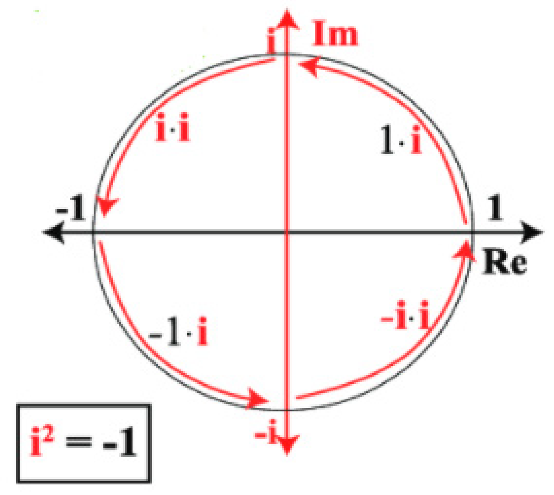
([16]). A CIFS ${\tilde{\Xi }}_{CI}$ is demonstrated by: 

$${\tilde{\Xi }}_{CI}=\{\left({\mu }_{{\tilde{\Xi }}_{CI}}\left(\stackrel{⌣}{\mathcal{x}}\right),{\eta }_{{\tilde{\Xi }}_{CI}}\left(\stackrel{⌣}{\mathcal{x}}\right)\right):\stackrel{⌣}{x}\in \overbrace{{\mathcal{X}}_{UNI}}\}$$

(1)

where ${\mu }_{{\tilde{\Xi }}_{CI}}={\mu }_{{\tilde{\Xi }}_{RP}}{e}^{i2\pi \left({\mu }_{{\tilde{\Xi }}_{IP}}\right)}$ and ${\eta }_{{\tilde{\Xi }}_{CI}}={\eta }_{{\tilde{\Xi }}_{RP}}{e}^{i2\pi \left({\eta }_{{\tilde{\Xi }}_{IP}}\right)}$ where $0\le {\mu }_{{\tilde{\Xi }}_{RP}}+{\eta }_{{\tilde{\Xi }}_{RP}}\le 1$ and $0\le {\mu }_{{\tilde{\Xi }}_{IP}}+{\eta }_{{\tilde{\Xi }}_{IP}}\le 1$. Furthermore, the refusal grade is demonstrated in the form of ${ℒ}_{{\tilde{\Xi }}_{CI}}={ℒ}_{{\tilde{\Xi }}_{RP}}{e}^{i2\pi \left({ℒ}_{{\tilde{\Xi }}_{IP}}\right)}=\left(1-{\mu }_{{\tilde{\Xi }}_{RP}}-{\eta }_{{\tilde{\Xi }}_{RP}}\right)e^{i2\pi \left(1-{\mu }_{{\tilde{\Xi }}_{RP}}-{\eta }_{{\tilde{\Xi }}_{RP}}\right)}$. In the overall manuscript, the complex intuitionistic fuzzy numbers (CIFNs) are represented by: ${\tilde{\Xi }}_{CI-i}=\left({\mu }_{{\tilde{\Xi }}_{RP-i}}{e}^{i2\pi \left({\mu }_{{\tilde{\Xi }}_{IP-i}}\right)},{\eta }_{{\tilde{\Xi }}_{RP-i}}{e}^{i2\pi \left({\eta }_{{\tilde{\Xi }}_{IP-i}}\right)}\right),i=1,2,\dots ,\overbrace{n}$. To determine the relationship among any number of attributes, the operations of addition, multiplication, and scaler multiplication and vector power scaler are discussed below. The graphical expressions of the unit disc are explained in Figure 1.

Definition 3

([17]). By using two CIFNs ${\tilde{\Xi }}_{CI-i}=\left({\mu }_{{\tilde{\Xi }}_{RP-i}}{e}^{i2\pi \left({\mu }_{{\tilde{\Xi }}_{IP-i}}\right)},{\eta }_{{\tilde{\Xi }}_{RP-i}}{e}^{i2\pi \left({\eta }_{{\tilde{\Xi }}_{IP-i}}\right)}\right),i=1,2$, then

$${\tilde{\Xi }}_{CI-1}⨁{\tilde{\Xi }}_{CI-2}=\left(\begin{array}{c}\left({\mu }_{{\tilde{\Xi }}_{RP-1}}+{\mu }_{{\tilde{\Xi }}_{RP-2}}-{\mu }_{{\tilde{\Xi }}_{RP-1}}{\mu }_{{\tilde{\Xi }}_{RP-2}}\right)e^{i2\pi \left({\mu }_{{\tilde{\Xi }}_{IP-1}}+{\mu }_{{\tilde{\Xi }}_{IP-2}}-{\mu }_{{\tilde{\Xi }}_{IP-1}}{\mu }_{{\tilde{\Xi }}_{IP-2}}\right)},\\ {\eta }_{{\tilde{\Xi }}_{RP-1}}{\eta }_{{\tilde{\Xi }}_{RP-2}}{e}^{i2\pi \left({\eta }_{{\tilde{\Xi }}_{IP-1}}{\eta }_{{\tilde{\Xi }}_{IP-2}}\right)}\end{array}\right)$$

(2)

$${\tilde{\Xi }}_{CI-1}⨂{\tilde{\Xi }}_{CI-2}=\left(\begin{array}{c}{\mu }_{{\tilde{\Xi }}_{RP-1}}{\mu }_{{\tilde{\Xi }}_{RP-2}}{e}^{i2\pi \left({\mu }_{{\tilde{\Xi }}_{IP-1}}{\mu }_{{\tilde{\Xi }}_{IP-2}}\right)},\\ \left({\eta }_{{\tilde{\Xi }}_{RP-1}}+{\eta }_{{\tilde{\Xi }}_{RP-2}}-{\eta }_{{\tilde{\Xi }}_{RP-1}}{\eta }_{{\tilde{\Xi }}_{RP-2}}\right)e^{i2\pi \left({\eta }_{{\tilde{\Xi }}_{IP-1}}+{\eta }_{{\tilde{\Xi }}_{IP-2}}-{\eta }_{{\tilde{\Xi }}_{IP-1}}{\eta }_{{\tilde{\Xi }}_{IP-2}}\right)}\end{array}\right)$$

(3)

$${\mathsf{\Phi }}_{SC}{\tilde{\Xi }}_{CI-1}=\left(\left(1-{\left(1-{\mu }_{{\tilde{\Xi }}_{RP-1}}\right)}^{{\mathsf{\Phi }}_{SC}}\right)e^{i2\pi \left(1-{\left(1-{\mu }_{{\tilde{\Xi }}_{IP-1}}\right)}^{{\mathsf{\Phi }}_{SC}}\right)},{\eta }_{{\tilde{\Xi }}_{RP-1}}^{{\mathsf{\Phi }}_{SC}}{e}^{i2\pi \left({\eta }_{{\tilde{\Xi }}_{IP-1}}^{{\mathsf{\Phi }}_{SC}}\right)}\right)$$

(4)

$${\tilde{\Xi }}_{CI-1}^{{\mathsf{\Phi }}_{SC}}=\left({\mu }_{{\tilde{\Xi }}_{RP-1}}^{{\mathsf{\Phi }}_{SC}}{e}^{i2\pi \left({\mu }_{{\tilde{\Xi }}_{IP-1}}^{{\mathsf{\Phi }}_{SC}}\right)},\left(1-{\left(1-{\eta }_{{\tilde{\Xi }}_{RP-1}}\right)}^{{\mathsf{\Phi }}_{SC}}\right)e^{i2\pi \left(1-{\left(1-{\eta }_{{\tilde{\Xi }}_{IP-1}}\right)}^{{\mathsf{\Phi }}_{SC}}\right)}\right)$$

(5)

To find the order between any two CIFS, we review the idea of score value (SV) and accuracy value (AV) based on CIFS, which are illustrated below. Without SV and AV, it is difficult to compare the CIFSs.

Definition 4

([17]). For two CIFNs ${\tilde{\Xi }}_{CI-i}=\left({\mu }_{{\tilde{\Xi }}_{RP-i}}{e}^{i2\pi \left({\mu }_{{\tilde{\Xi }}_{IP-i}}\right)},{\eta }_{{\tilde{\Xi }}_{RP-i}}{e}^{i2\pi \left({\eta }_{{\tilde{\Xi }}_{IP-i}}\right)}\right),i=1$, the score value (SV) and accuracy value (AV) are demonstrated as: 

$${\mathbb{S}}_{SV}\left({\tilde{\Xi }}_{CI-1}\right)=\frac{1}{2}\left({\mu }_{{\tilde{\Xi }}_{RP-1}}+{\mu }_{{\tilde{\Xi }}_{RP-2}}-{\eta }_{{\tilde{\Xi }}_{RP-1}}-{\eta }_{{\tilde{\Xi }}_{RP-1}}\right)$$

(6)

$${ℍ}_{AV}\left({\tilde{\Xi }}_{CI-1}\right)=\frac{1}{2}\left({\mu }_{{\tilde{\Xi }}_{RP-1}}+{\mu }_{{\tilde{\Xi }}_{RP-2}}+{\eta }_{{\tilde{\Xi }}_{RP-1}}+{\eta }_{{\tilde{\Xi }}_{RP-1}}\right)$$

(7)

By using the above information, we can determine which CIFN is superior and which one is inferior, for this purpose we must revise the rules for comparison between any number of CIFNs such as:

• When ${\mathbb{S}}_{SV}\left({\tilde{\Xi }}_{CI-1}\right)>{\mathbb{S}}_{SV}\left({\tilde{\Xi }}_{CI-2}\right)⟹{\tilde{\Xi }}_{CI-1}>{\tilde{\Xi }}_{CI-2}$;
• When ${\mathbb{S}}_{SV}\left({\tilde{\Xi }}_{CI-1}\right)={\mathbb{S}}_{SV}\left({\tilde{\Xi }}_{CI-2}\right)⟹$

  (1)

  When ${ℍ}_{AV}\left({\tilde{\Xi }}_{CI-1}\right)={ℍ}_{AV}\left({\tilde{\Xi }}_{CI-2}\right)⟹{\tilde{\Xi }}_{CI-1}={\tilde{\Xi }}_{CI-2}$.

  (2)

  When ${ℍ}_{AV}\left({\tilde{\Xi }}_{CI-1}\right)={ℍ}_{AV}\left({\tilde{\Xi }}_{CI-2}\right)⟹{\tilde{\Xi }}_{CI-1}={\tilde{\Xi }}_{CI-2}$.

To determine the exact value from the group of values, the aggregation operators are more flexible and more dominant to find the reliability and consistency in genuine life troubles. The prioritized aggregation operator is one of the most important and dominant parts of the operators that perform mathematical operations, such as Average, Aggregate, Count, Max, Min, and Sum, on the numeric property of the elements in the collection.

Definition 5

([27]). By using any numbers of positive integers ${\tilde{\Xi }}_{CI-i},i=1,2,\dots ,\overbrace{n}$, the PWA operator is demonstrated by:

$$PWA\left({\tilde{\Xi }}_{CI-1},{\tilde{\Xi }}_{CI-2},\dots ,{\tilde{\Xi }}_{CI-\overbrace{n}}\right)={\displaystyle \sum }_{i=1}^{\overbrace{n}}\frac{{\mathcal{Z}}_i}{{{\displaystyle \sum }}_{i=1}^{\overbrace{n}}{\mathcal{Z}}_i}$$

(8)

where ${\mathcal{Z}}_1=1$, with

$${\mathcal{Z}}_i={\displaystyle \prod }_{k=1}^{i-1}{\tilde{\Xi }}_{CI-k}$$

(9)

Definition 6

([32]). A CIFSS ${\tilde{\Xi }}_{CI}:ℰ⟶CIFS\left(\overbrace{{\mathcal{X}}_{UNI}}\right)$ is demonstrated by:

$$\left({\tilde{\Xi }}_{CI}, ℰ\right)=\left\{\left(x_i,{\tilde{\Xi }}_{CI-e_j}\left({\stackrel{⌣}{x}}_i\right)\right):\stackrel{⌣}{x_l}\in \overbrace{{\mathcal{X}}_{UNI}}\right\}$$

(10)

Definition 7

([33]). A CIFSS ${\tilde{\Xi }}_{CI}:ℰ⟶CIFS\left(\overbrace{{\mathcal{X}}_{UNI}}\right)$ is demonstrated by:

$${\tilde{\Xi }}_{CI}\left(e\right)=\left\{\left({\mu }_{{\tilde{\Xi }}_{RP-j}}\left(\stackrel{⌣}{x_l}\right)e^{i\left({\mu }_{{\tilde{\Xi }}_{IP-j}}\left(\stackrel{⌣}{x_l}\right)\right)},{\eta }_{{\tilde{\Xi }}_{RP-j}}\left(\stackrel{⌣}{x_l}\right)e^{i\left({\eta }_{{\tilde{\Xi }}_{IP-j}}\left(\stackrel{⌣}{x_l}\right)\right)}\right):\stackrel{⌣}{x_l}\in \overbrace{{\mathcal{X}}_{UNI}}\right\}$$

(11)

where ${\mu }_{{\tilde{\Xi }}_{IP-j}}\left(\stackrel{⌣}{x_l}\right),{\eta }_{{\tilde{\Xi }}_{IP-j}}\left(\stackrel{⌣}{x_l}\right)\in \left[0,2\pi \right]$. The ideas in Equations (10) and (11), encompass some problems related to imaginary parts and their conditions. Similarly, no one elaborated on the operational laws or score value and accuracy value, which are very useful and important for developing aggregation operators. To resolve the above troubles, in the next study, we elaborated on the idea of CIFSSs with the new structure and utilized their operational laws.

3. A Novel Complex Intuitionistic Fuzzy Soft Set

In this study, we will improve the existing principle of CIFSSs and elaborate on their new fundamental laws. The proposed work is also justified with the help of some numerical examples to show the reliability and effectiveness of the presented work. The existing CIFSSs were explored by Kumar and Bajaj [32] and Quek et al. [33]. Based on the above existing ideas, the novel approach is discussed below.

Definition 8.

A CIFSS ${\tilde{\Xi }}_{CI}:ℰ⟶CIFS\left(\overbrace{{\mathcal{X}}_{UNI}}\right)$ is demonstrated by:

$${\tilde{\Xi }}_{CI-e_j}\left({\stackrel{⌣}{x}}_i\right)=\left\{\left({\mu }_{{\tilde{\Xi }}_{CI-j}}\left(\stackrel{⌣}{x_l}\right),{\eta }_{{\tilde{\Xi }}_{CI-j}}\left(\stackrel{⌣}{x_l}\right)\right):\stackrel{⌣}{x_l}\in \overbrace{{\mathcal{X}}_{UNI}}\right\}$$

(12)

where ${\mu }_{{\tilde{\Xi }}_{CI-j}}\left(\stackrel{⌣}{x_l}\right)={\mu }_{{\tilde{\Xi }}_{RP-j}}\left(\stackrel{⌣}{x_l}\right)e^{i2\pi \left({\mu }_{{\tilde{\Xi }}_{IP-j}}\left(\stackrel{⌣}{x_l}\right)\right)}$ and ${\eta }_{{\tilde{\Xi }}_{CI-j}}\left(\stackrel{⌣}{x_l}\right)={\eta }_{{\tilde{\Xi }}_{RP-j}}\left(\stackrel{⌣}{x_l}\right)e^{i2\pi \left({\eta }_{{\tilde{\Xi }}_{IP-j}}\left(\stackrel{⌣}{x_l}\right)\right)}$ with the rules such that $0\le {\mu }_{{\tilde{\Xi }}_{RP-j}}\left(\stackrel{⌣}{x_l}\right)+{\eta }_{{\tilde{\Xi }}_{RP-j}}\left(\stackrel{⌣}{x_l}\right)\le 1$ and $0\le {\mu }_{{\tilde{\Xi }}_{IP-j}}\left(\stackrel{⌣}{x_l}\right)+{\eta }_{{\tilde{\Xi }}_{IP-j}}\left(\stackrel{⌣}{x_l}\right)\le 1$. Furthermore, the term ${ℒ}_{{\tilde{\Xi }}_{CI-j}}\left(\stackrel{⌣}{x_l}\right)={ℒ}_{{\tilde{\Xi }}_{RP-j}}\left(\stackrel{⌣}{x_l}\right)e^{i2\pi \left({ℒ}_{{\tilde{\Xi }}_{IP-j}}\left(\stackrel{⌣}{x_l}\right)\right)}=\left(1-{\mu }_{{\tilde{\Xi }}_{RP-j}}\left(\stackrel{⌣}{x_l}\right)-{\eta }_{{\tilde{\Xi }}_{RP-j}}\left(\stackrel{⌣}{x_l}\right)\right)e^{i2\pi \left(1-{\mu }_{{\tilde{\Xi }}_{RP-j}}\left(\stackrel{⌣}{x_l}\right)-{\eta }_{{\tilde{\Xi }}_{RP-j}}\left(\stackrel{⌣}{x_l}\right)\right)}$ expresses the refusal grade. Where the symbol $CIFS\left(\overbrace{{\mathcal{X}}_{UNI}}\right)$ expresses the family of CQROFNs. Throughout this manuscript, the complex intuitionistic fuzzy soft number (CIFSN) is expressed by: ${\tilde{\Xi }}_{CI-e_{ij}}=\left({\mu }_{{\tilde{\Xi }}_{RP-ij}}{e}^{i2\pi \left({\mu }_{{\tilde{\Xi }}_{IP-ij}}\right)},{\eta }_{{\tilde{\Xi }}_{RP-ij}}{e}^{i2\pi \left({\eta }_{{\tilde{\Xi }}_{IP-ij}}\right)}\right),i,j=1,2,\dots ,\overbrace{n},\overbrace{m}$.

Example 1.

Among the main applications of radiophysics are radio communications, radiolocation, radio astronomy, and radiology. Classical radiophysics deals with radio wave communications and detection. This well-known experience of actual application of complex numbers in radiophysics, optics, and energy systems naturally anticipates oscillating and periodic time parameters for complex models of decision making and is more suitable for the complex module. For this, we choose the family of a fixed set $\overbrace{{\mathcal{X}}_{UNI}}=\left\{\stackrel{⌣}{x_1},\stackrel{⌣}{x_2},\stackrel{⌣}{x_3},\stackrel{⌣}{x_4}\right\}$ and corresponding of parameters $ℰ=\left\{e_1\left(Expensive\right),e_2\left(Wooden\right),e_3\left(Cheap\right),e_4\left(Beautiful\right),e_5\left(In good location\right)\right\}$, then the rating values of each value of the fix set concerning parameters are discussed in

Table 1. Expressions of the complex intuitionistic fuzzy soft numbers.

${\tilde{\mathit{\Xi }}}_{\mathit{C}\mathit{I}}$	${\mathit{e}}_1$	${\mathit{e}}_2$	${\mathit{e}}_3$	${\mathit{e}}_4$	${\mathit{e}}_5$
$\stackrel{\mathbf{⌣}}{{\mathit{x}}_{\mathbf{1}}}$	$\left(\begin{array}{c}0.2e^{i2\pi \left(0.2\right)},\\ 0.6e^{i2\pi \left(0.6\right)}\end{array}\right)$	$\left(\begin{array}{c}0.1e^{i2\pi \left(0.1\right)},\\ 0.5e^{i2\pi \left(0.5\right)}\end{array}\right)$	$\left(\begin{array}{c}0.9e^{i2\pi \left(0.9\right)},\\ 0.1e^{i2\pi \left(0.1\right)}\end{array}\right)$	$\left(\begin{array}{c}0.3e^{i2\pi \left(0.3\right)},\\ 0.4e^{i2\pi \left(0.4\right)}\end{array}\right)$	$\left(\begin{array}{c}0.6e^{i2\pi \left(0.6\right)},\\ 0.2e^{i2\pi \left(0.2\right)}\end{array}\right)$
$\stackrel{\mathbf{⌣}}{{\mathit{x}}_{\mathbf{2}}}$	$\left(\begin{array}{c}0.5e^{i2\pi \left(0.5\right)},\\ 0.4e^{i2\pi \left(0.4\right)}\end{array}\right)$	$\left(\begin{array}{c}0.2e^{i2\pi \left(0.2\right)},\\ 0.5e^{i2\pi \left(0.5\right)}\end{array}\right)$	$\left(\begin{array}{c}0.3e^{i2\pi \left(0.3\right)},\\ 0.7e^{i2\pi \left(0.7\right)}\end{array}\right)$	$\left(\begin{array}{c}0.6e^{i2\pi \left(0.6\right)},\\ 0.2e^{i2\pi \left(0.2\right)}\end{array}\right)$	$\left(\begin{array}{c}0.4e^{i2\pi \left(0.4\right)},\\ 0.4e^{i2\pi \left(0.4\right)}\end{array}\right)$
$\stackrel{\mathbf{⌣}}{{\mathit{x}}_{\mathbf{3}}}$	$\left(\begin{array}{c}0.6e^{i2\pi \left(0.6\right)},\\ 0.2e^{i2\pi \left(0.2\right)}\end{array}\right)$	$\left(\begin{array}{c}0.5e^{i2\pi \left(0.5\right)},\\ 0.4e^{i2\pi \left(0.4\right)}\end{array}\right)$	$\left(\begin{array}{c}0.8e^{i2\pi \left(0.8\right)},\\ 0.1e^{i2\pi \left(0.1\right)}\end{array}\right)$	$\left(\begin{array}{c}0.6e^{i2\pi \left(0.6\right)},\\ 0.4e^{i2\pi \left(0.4\right)}\end{array}\right)$	$\left(\begin{array}{c}0.2e^{i2\pi \left(0.2\right)},\\ 0.7e^{i2\pi \left(0.7\right)}\end{array}\right)$
$\stackrel{\mathbf{⌣}}{{\mathit{x}}_{\mathbf{4}}}$	$\left(\begin{array}{c}0.4e^{i2\pi \left(0.4\right)},\\ 0.5e^{i2\pi \left(0.5\right)}\end{array}\right)$	$\left(\begin{array}{c}0.3e^{i2\pi \left(0.3\right)},\\ 0.5e^{i2\pi \left(0.5\right)}\end{array}\right)$	$\left(\begin{array}{c}0.6e^{i2\pi \left(0.6\right)},\\ 0.1e^{i2\pi \left(0.1\right)}\end{array}\right)$	$\left(\begin{array}{c}0.4e^{i2\pi \left(0.4\right)},\\ 0.1e^{i2\pi \left(0.1\right)}\end{array}\right)$	$\left(\begin{array}{c}0.2e^{i2\pi \left(0.2\right)},\\ 0.4e^{i2\pi \left(0.4\right)}\end{array}\right)$

.

In the procedure to utilize the CQROFSSs in realistic troubles, it is necessary to determine the ranking of these all numbers. For this, we develop the SV and AV, demonstrated below.

Definition 9.

For the CIFSNs, ${\tilde{\Xi }}_{CI-e_{ij}}=\left({\mu }_{{\tilde{\Xi }}_{RP-ij}}{e}^{i2\pi \left({\mu }_{{\tilde{\Xi }}_{IP-ij}}\right)},{\eta }_{{\tilde{\Xi }}_{RP-ij}}{e}^{i2\pi \left({\eta }_{{\tilde{\Xi }}_{IP-ij}}\right)}\right),i,j=1,2,\dots ,\overbrace{n},\overbrace{m}$ their SV and AV are demonstrated by:

$${\mathbb{S}}_{SV}\left({\tilde{\Xi }}_{CI-e_{ij}}\right)=\frac{1}{4}\left(1+{\mu }_{{\tilde{\Xi }}_{RP-ij}}+{\mu }_{{\tilde{\Xi }}_{RP-ij}}-{\eta }_{{\tilde{\Xi }}_{RP-ij}}-{\eta }_{{\tilde{\Xi }}_{RP-ij}}\right)$$

(13)

$${ℍ}_{AV}\left({\tilde{\Xi }}_{CI-e_{ij}}\right)=\frac{1}{4}\left(1+{\mu }_{{\tilde{\Xi }}_{RP-ij}}+{\mu }_{{\tilde{\Xi }}_{RP-ij}}+{\eta }_{{\tilde{\Xi }}_{RP-ij}}+{\eta }_{{\tilde{\Xi }}_{RP-ij}}\right)$$

(14)

By using the above information, we can determine which CIFSN is superior and which one is inferior. We, thus, revise the rules for the comparison between any number of CIFSNs such as:

• When ${\mathbb{S}}_{SV}\left({\tilde{\Xi }}_{CI-e_{ij}}\right)>{\mathbb{S}}_{SV}\left({\widetilde{{\Xi }^{\prime }}}_{CI-e_{ij}}\right)⟹{\tilde{\Xi }}_{CI-e_{ij}}>{\widetilde{{\Xi }^{\prime }}}_{CI-e_{ij}}$;
• When ${\mathbb{S}}_{SV}\left({\tilde{\Xi }}_{CI-e_{ij}}\right)={\mathbb{S}}_{SV}\left({\widetilde{{\Xi }^{\prime }}}_{CI-e_{ij}}\right)⟹$

  (1)

  When ${ℍ}_{AV}\left({\tilde{\Xi }}_{CI-e_{ij}}\right)>{ℍ}_{AV}\left({\widetilde{{\Xi }^{\prime }}}_{CI-e_{ij}}\right)⟹{\tilde{\Xi }}_{CI-e_{ij}}>{\widetilde{{\Xi }^{\prime }}}_{CI-e_{ij}}$;

  (2)

  When ${ℍ}_{AV}\left({\tilde{\Xi }}_{CI-e_{ij}}\right)={ℍ}_{AV}\left({\widetilde{{\Xi }^{\prime }}}_{CI-e_{ij}}\right)⟹{\tilde{\Xi }}_{CI-e_{ij}}={\widetilde{{\Xi }^{\prime }}}_{CI-e_{ij}}$.

Definition 10.

By using two CIFSNs ${\tilde{\Xi }}_{CI-e_{11}}=\left({\mu }_{{\tilde{\Xi }}_{RP-11}}{e}^{i2\pi \left({\mu }_{{\tilde{\Xi }}_{IP-11}}\right)},{\eta }_{{\tilde{\Xi }}_{RP-11}}{e}^{i2\pi \left({\eta }_{{\tilde{\Xi }}_{IP-11}}\right)}\right)$ and ${\tilde{\Xi }}_{CI-e_{12}}=\left({\mu }_{{\tilde{\Xi }}_{RP-12}}{e}^{i2\pi \left({\mu }_{{\tilde{\Xi }}_{IP-12}}\right)},{\eta }_{{\tilde{\Xi }}_{RP-12}}{e}^{i2\pi \left({\eta }_{{\tilde{\Xi }}_{IP-12}}\right)}\right)$, then

$${\tilde{\Xi }}_{CI-e_{11}}⨁{\tilde{\Xi }}_{CI-e_{12}}=\left(\begin{array}{c}\left({\mu }_{{\tilde{\Xi }}_{RP-11}}+{\mu }_{{\tilde{\Xi }}_{RP-12}}-{\mu }_{{\tilde{\Xi }}_{RP-11}}{\mu }_{{\tilde{\Xi }}_{RP-12}}\right)e^{i2\pi \left({\mu }_{{\tilde{\Xi }}_{IP-11}}+{\mu }_{{\tilde{\Xi }}_{IP-12}}-{\mu }_{{\tilde{\Xi }}_{IP-11}}{\mu }_{{\tilde{\Xi }}_{IP-12}}\right)},\\ {\eta }_{{\tilde{\Xi }}_{RP-11}}{\eta }_{{\tilde{\Xi }}_{RP-12}}{e}^{i2\pi \left({\eta }_{{\tilde{\Xi }}_{IP-11}}{\eta }_{{\tilde{\Xi }}_{IP-12}}\right)}\end{array}\right)$$

(15)

$${\tilde{\Xi }}_{CI-e_{11}}⨂{\tilde{\Xi }}_{CI-{ℯ}_{12}}=\left(\begin{array}{c}{\mu }_{{\tilde{\Xi }}_{RP-11}}{\mu }_{{\tilde{\Xi }}_{RP-12}}{e}^{i2\pi \left({\mu }_{{\tilde{\Xi }}_{IP-11}}{\mu }_{{\tilde{\Xi }}_{IP-12}}\right)},\\ \left({\eta }_{{\tilde{\Xi }}_{RP-11}}+{\eta }_{{\tilde{\Xi }}_{RP-12}}-{\eta }_{{\tilde{\Xi }}_{RP-11}}{\eta }_{{\tilde{\Xi }}_{RP-12}}\right)e^{i2\pi \left({\eta }_{{\tilde{\Xi }}_{IP-11}}+{\eta }_{{\tilde{\Xi }}_{IP-12}}-{\eta }_{{\tilde{\Xi }}_{IP-11}}{\eta }_{{\tilde{\Xi }}_{IP-12}}\right)}\end{array}\right)$$

(16)

$${\mathsf{\Phi }}_{SC}{\tilde{\Xi }}_{CI-e_{11}}=\left(\left(1-{\left(1-{\mu }_{{\tilde{\Xi }}_{RP-11}}\right)}^{{\mathsf{\Phi }}_{SC}}\right)e^{i2\pi \left(1-{\left(1-{\mu }_{{\tilde{\Xi }}_{IP-11}}\right)}^{{\mathsf{\Phi }}_{SC}}\right)},{\eta }_{{\tilde{\Xi }}_{RP-11}}^{{\mathsf{\Phi }}_{SC}}{e}^{i2\pi \left({\eta }_{{\tilde{\Xi }}_{IP-11}}^{{\mathsf{\Phi }}_{SC}}\right)}\right)$$

(17)

$${\tilde{\Xi }}_{CI-e_{11}}^{{\mathsf{\Phi }}_{SC}}=\left({\mu }_{{\tilde{\Xi }}_{RP-11}}^{{\mathsf{\Phi }}_{SC}}{e}^{i2\pi \left({\mu }_{{\tilde{\Xi }}_{IP-11}}^{{\mathsf{\Phi }}_{SC}}\right)},\left(1-{\left(1-{\eta }_{{\tilde{\Xi }}_{RP-11}}\right)}^{{\mathsf{\Phi }}_{SC}}\right)e^{i2\pi \left(1-{\left(1-{\eta }_{{\tilde{\Xi }}_{IP-11}}\right)}^{{\mathsf{\Phi }}_{SC}}\right)}\right)$$

(18)

Theorem 1.

By using CIFSNs ${\tilde{\Xi }}_{CI-e_{ij}}=\left({\mu }_{{\tilde{\Xi }}_{RP-ij}}{e}^{i2\pi \left({\mu }_{{\tilde{\Xi }}_{IP-ij}}\right)},{\eta }_{{\tilde{\Xi }}_{RP-ij}}{e}^{i2\pi \left({\eta }_{{\tilde{\Xi }}_{IP-ij}}\right)}\right),i,j=1,2,\dots ,\overbrace{n},\overbrace{m}$, then

• ${\tilde{\Xi }}_{CI-e_{11}}⨁{\tilde{\Xi }}_{CI-e_{12}}={\tilde{\Xi }}_{CI-e_{12}}⨁{\tilde{\Xi }}_{CI-e_{11}}$;
• ${\tilde{\Xi }}_{CI-e_{11}}⨂{\tilde{\Xi }}_{CI-e_{12}}={\tilde{\Xi }}_{CI-e_{12}}⨂{\tilde{\Xi }}_{CI-e_{11}}$;
• $\left({\tilde{\Xi }}_{CI-e_{11}}⨁{\tilde{\Xi }}_{CI-e_{12}}\right)⨁{\tilde{\Xi }}_{CI-e_{13}}={\tilde{\Xi }}_{CI-e_{12}}⨁\left({\tilde{\Xi }}_{CI-e_{11}}⨁{\tilde{\Xi }}_{CI-e_{13}}\right)$;
• $\left({\tilde{\Xi }}_{CI-e_{11}}⨂{\tilde{\Xi }}_{CI-e_{12}}\right)⨂{\tilde{\Xi }}_{CI-e_{13}}={\tilde{\Xi }}_{CI-e_{12}}⨂\left({\tilde{\Xi }}_{CI-e_{11}}⨂{\tilde{\Xi }}_{CI-e_{13}}\right)$;
• ${\mathsf{\Phi }}_{SC}\left({\tilde{\Xi }}_{CI-e_{11}}⨁{\tilde{\Xi }}_{CI-e_{12}}\right)={\mathsf{\Phi }}_{SC}{\tilde{\Xi }}_{CI-e_{11}}⨁{\mathsf{\Phi }}_{SC}{\tilde{\Xi }}_{CI-e_{12}}$;
• ${\left({\tilde{\Xi }}_{CI-e_{11}}⨂{\tilde{\Xi }}_{CI-e_{12}}\right)}^{{\mathsf{\Phi }}_{SC}}={\tilde{\Xi }}_{CI-e_{11}}^{{\mathsf{\Phi }}_{SC}}⨂{\tilde{\Xi }}_{CI-e_{12}}^{{\mathsf{\Phi }}_{SC}}$;
• ${\mathsf{\Phi }}_{SC-1}{\tilde{\Xi }}_{CI-e_{11}}⨁{\mathsf{\Phi }}_{SC-2}{\tilde{\Xi }}_{CI-e_{11}}=\left({\mathsf{\Phi }}_{SC-1}+{\mathsf{\Phi }}_{SC-2}\right){\tilde{\Xi }}_{CI-e_{11}}$;
• ${\tilde{\Xi }}_{CI-e_{11}}^{{\mathsf{\Phi }}_{SC-1}}⨂{\tilde{\Xi }}_{CI-e_{11}}^{{\mathsf{\Phi }}_{SC-2}}={\tilde{\Xi }}_{CI-e_{11}}^{\left({\mathsf{\Phi }}_{SC-1}+{\mathsf{\Phi }}_{SC-2}\right)}$.

Proof. 

Trivial. □

4. Averaging and Geometric Prioritized Aggregation Operators

As shown above, to find the relationship among any number of attributes the aggregation operators are one the best technique to determine the consistency of the elaborated operators. By using the advantages of the elaborated CIFSSs, in this study, we elaborated on CIFSPWAO, CIFSPOWAO, CIFSPWGO, and CIFSPOWGO, and deliberated their properties.

Definition 11.

For the CIFSNs ${\tilde{\Xi }}_{CI-e_{ij}}=\left({\mu }_{{\tilde{\Xi }}_{RP-ij}}{e}^{i2\pi \left({\mu }_{{\tilde{\Xi }}_{IP-ij}}\right)},{\eta }_{{\tilde{\Xi }}_{RP-ij}}{e}^{i2\pi \left({\eta }_{{\tilde{\Xi }}_{IP-ij}}\right)}\right),i,j=1,2,\dots ,\overbrace{n},\overbrace{m}$, their CIFSPWA operators are demonstrated by:

$$CIFSPWA\left({\tilde{\Xi }}_{CI-e_{11}},{\tilde{\Xi }}_{CI-e_{12}},\dots ,{\tilde{\Xi }}_{CI-e_{\overbrace{m}\overbrace{n}}}\right)={\oplus }_{i=1}^{\overbrace{m}}\frac{{\mathcal{Z}}_i}{{{\displaystyle \sum }}_{i=1}^{\overbrace{m}}{\mathcal{Z}}_i}\left({\oplus }_{j=1}^{\overbrace{n}}\frac{{ℨ}_j}{{{\displaystyle \sum }}_{j=1}^{\overbrace{n}}{ℨ}_j}{\tilde{\Xi }}_{CI-e_{ij}}\right)$$

(19)

where ${ℨ}_1={\mathcal{Z}}_1=1$ and

$${ℨ}_j={\displaystyle \prod }_{l=1}^{j-1}{\mathbb{S}}_{SV}\left({\tilde{\Xi }}_{CI-l}\right),j=1,2,\dots ,\overbrace{n}$$

(20)

$${\mathcal{Z}}_i={\displaystyle \prod }_{k=1}^{i-1}{\mathbb{S}}_{SV}\left({\tilde{\Xi }}_{CI-k}\right),i,j=1,2,\dots ,\overbrace{m}$$

(21)

By using Definition 11, we utilized the following results.

Theorem 2.

For the CIFSNs ${\tilde{\Xi }}_{CI-e_{ij}}=\left({\mu }_{{\tilde{\Xi }}_{RP-ij}}{e}^{i2\pi \left({\mu }_{{\tilde{\Xi }}_{IP-ij}}\right)},{\eta }_{{\tilde{\Xi }}_{RP-ij}}{e}^{i2\pi \left({\eta }_{{\tilde{\Xi }}_{IP-ij}}\right)}\right),i,j=1,2,\dots ,\overbrace{n},\overbrace{m}$, thereby using Equation (19), we have

$$CIFSPWA\left({\tilde{\Xi }}_{CI-e_{11}},{\tilde{\Xi }}_{CI-e_{12}},\dots ,{\tilde{\Xi }}_{CI-e_{\overbrace{m}\overbrace{n}}}\right)=\left(\begin{array}{c}{(1-{\displaystyle {\displaystyle \prod }_{i=1}^{\overbrace{m}}}{\left({\displaystyle {\displaystyle \prod }_{j=1}^{\overbrace{n}}}{\left(1-{\mu }_{{\tilde{\Xi }}_{RP-ij}}\right)}^{\frac{{ℨ}_j}{{{\displaystyle \sum }}_{j=1}^{\overbrace{n}}{ℨ}_j}}\right)}^{\frac{{\mathcal{Z}}_i}{{{\displaystyle \sum }}_{i=1}^{\overbrace{m}}{\mathcal{Z}}_i}})e}^{i2\pi \left(1-{{\displaystyle \prod }}_{i=1}^{\overbrace{m}}{\left({{\displaystyle \prod }}_{j=1}^{\overbrace{n}}{\left(1-{\mu }_{{\tilde{\Xi }}_{IP-ij}}\right)}^{\frac{{ℨ}_j}{{{\displaystyle \sum }}_{j=1}^{\overbrace{n}}{ℨ}_j}}\right)}^{\frac{{\mathcal{Z}}_i}{{{\displaystyle \sum }}_{i=1}^{\overbrace{m}}{\mathcal{Z}}_i}}\right)},\\ {\displaystyle {\displaystyle \prod }_{i=1}^{\overbrace{m}}}{\left({\displaystyle {\displaystyle \prod }_{j=1}^{\overbrace{n}}}{\eta }_{{\tilde{\Xi }}_{RP-ij}}{}^{\frac{{ℨ}_j}{{{\displaystyle \sum }}_{j=1}^{\overbrace{n}}{ℨ}_j}}\right)}^{\frac{{\mathcal{Z}}_i}{{{\displaystyle \sum }}_{i=1}^{\overbrace{m}}{\mathcal{Z}}_i}}{e}^{i2\pi \left({{\displaystyle \prod }}_{i=1}^{\overbrace{m}}{\left({{\displaystyle \prod }}_{j=1}^{\overbrace{n}}{\eta }_{{\tilde{\Xi }}_{IP-ij}}{}^{\frac{{ℨ}_j}{{{\displaystyle \sum }}_{j=1}^{\overbrace{n}}{ℨ}_j}}\right)}^{\frac{{\mathcal{Z}}_i}{{{\displaystyle \sum }}_{i=1}^{\overbrace{m}}{\mathcal{Z}}_i}}\right)}\end{array}\right)$$

(22)

Proof. 

See Appendix A. □

By using Theorem 2, we initiated the following properties such as idempotency, boundedness, and monotonicity.

Theorem 3.

For the CIFSNs ${\tilde{\Xi }}_{CI-e_{ij}}=\left({\mu }_{{\tilde{\Xi }}_{RP-ij}}{e}^{i2\pi \left({\mu }_{{\tilde{\Xi }}_{IP-ij}}\right)},{\eta }_{{\tilde{\Xi }}_{RP-ij}}{e}^{i2\pi \left({\eta }_{{\tilde{\Xi }}_{IP-ij}}\right)}\right),i,j=1,2,\dots ,\overbrace{n},\overbrace{m}$, if ${\tilde{\Xi }}_{CI-e_{ij}}={\tilde{\Xi }}_{CI-e}=\left({\mu }_{{\tilde{\Xi }}_{RP}}{e}^{i2\pi \left({\mu }_{{\tilde{\Xi }}_{IP}}\right)},{\eta }_{{\tilde{\Xi }}_{RP}}{e}^{i2\pi \left({\eta }_{{\tilde{\Xi }}_{IP}}\right)}\right)$, then

$$CIFSPWA\left({\tilde{\Xi }}_{CI-e_{11}},{\tilde{\Xi }}_{CI-e_{12}},\dots ,{\tilde{\Xi }}_{CI-e_{\overbrace{m}\overbrace{n}}}\right)={\tilde{\Xi }}_{CI-e}$$

(23)

Proof. 

See Appendix A. □

Theorem 4.

For the CIFSNs ${\tilde{\Xi }}_{CI-e_{ij}}=\left({\mu }_{{\tilde{\Xi }}_{RP-ij}}{e}^{i2\pi \left({\mu }_{{\tilde{\Xi }}_{IP-ij}}\right)},{\eta }_{{\tilde{\Xi }}_{RP-ij}}{e}^{i2\pi \left({\eta }_{{\tilde{\Xi }}_{IP-ij}}\right)}\right),i,j=1,2,\dots ,\overbrace{n},\overbrace{m}$, if ${\tilde{\Xi }}_{CI-e_{ij}}^{-}=\left(\underset{i}{min }\underset{j}{min }{\mu }_{{\tilde{\Xi }}_{RP-ij}}{e}^{i2\pi \left(\underset{i}{min }\underset{j}{min }{\mu }_{{\tilde{\Xi }}_{IP-ij}}\right)},\underset{i}{max }\underset{j}{max }{\eta }_{{\tilde{\Xi }}_{RP-ij}}{e}^{i2\pi \left(\underset{i}{max }\underset{j}{max }{\eta }_{{\tilde{\Xi }}_{RP-ij}}\right)}\right)$ and ${\tilde{\Xi }}_{CI-e_{ij}}^{+}=\left(\underset{i}{max }\underset{j}{max }{\mu }_{{\tilde{\Xi }}_{RP-ij}}{e}^{i2\pi \left(\underset{i}{max }\underset{j}{max }{\mu }_{{\tilde{\Xi }}_{IP-ij}}\right)},\underset{i}{min }\underset{j}{min }{\eta }_{{\tilde{\Xi }}_{RP-ij}}{e}^{i2\pi \left(\underset{i}{min }\underset{j}{min }{\eta }_{{\tilde{\Xi }}_{RP-ij}}\right)}\right)$, the

$${\tilde{\Xi }}_{CI-e_{ij}}^{-}\le CIFSPWA\left({\tilde{\Xi }}_{CI-e_{11}},{\tilde{\Xi }}_{CI-e_{12}},\dots ,{\tilde{\Xi }}_{CI-e_{\overbrace{m}\overbrace{n}}}\right)\le {\tilde{\Xi }}_{CI-e_{ij}}^{+}$$

(24)

Proof. 

See Appendix A. □

Theorem 5.

For the CIFSNs ${\tilde{\Xi }}_{CI-e_{ij}}=\left({\mu }_{{\tilde{\Xi }}_{RP-ij}}{e}^{i2\pi \left({\mu }_{{\tilde{\Xi }}_{IP-ij}}\right)},{\eta }_{{\tilde{\Xi }}_{RP-ij}}{e}^{i2\pi \left({\eta }_{{\tilde{\Xi }}_{IP-ij}}\right)}\right),i,j=1,2,\dots ,\overbrace{n},\overbrace{m}$, if ${\tilde{\Xi }}_{CI-e_{ij}}\le {\tilde{\Xi }}_{CI-e_{ij}}^{\prime }$, then

$$CIFSPWA\left({\tilde{\Xi }}_{CI-e_{11}},{\tilde{\Xi }}_{CI-e_{12}},\dots ,{\tilde{\Xi }}_{CI-e_{\overbrace{m}\overbrace{n}}}\right)\le CIFSPWA\left({\tilde{\Xi }}_{CI-e_{11}}^{\prime },{\tilde{\Xi }}_{CI-e_{12}}^{\prime },\dots ,{\tilde{\Xi }}_{CI-e_{\overbrace{m}\overbrace{n}}}^{\prime }\right)$$

(25)

Proof. 

The proof of this theorem is like the proof of Theorem 4. □

Definition 12.

For the CIFSNs ${\tilde{\Xi }}_{CI-e_{ij}}=\left({\mu }_{{\tilde{\Xi }}_{RP-ij}}{e}^{i2\pi \left({\mu }_{{\tilde{\Xi }}_{IP-ij}}\right)},{\eta }_{{\tilde{\Xi }}_{RP-ij}}{e}^{i2\pi \left({\eta }_{{\tilde{\Xi }}_{IP-ij}}\right)}\right),i,j=1,2,\dots ,\overbrace{n},\overbrace{m}$, their CIFSPOWA operators is demonstrated by:

$$CIFSPOWA\left({\tilde{\Xi }}_{CI-e_{11}},{\tilde{\Xi }}_{CI-e_{12}},\dots ,{\tilde{\Xi }}_{CI-e_{\overbrace{m}\overbrace{n}}}\right)={\oplus }_{i=1}^{\overbrace{m}}\frac{{\mathcal{Z}}_i}{{{\displaystyle \sum }}_{i=1}^{\overbrace{m}}{\mathcal{Z}}_i}\left({\oplus }_{j=1}^{\overbrace{n}}\frac{{ℨ}_j}{{{\displaystyle \sum }}_{j=1}^{\overbrace{n}}{ℨ}_j}{\tilde{\Xi }}_{CI-e_{\sigma \left(i\right)\sigma \left(j\right)}}\right)$$

(26)

where ${ℨ}_1={\mathcal{Z}}_1=1$ and

$${ℨ}_j={\displaystyle \prod }_{l=1}^{j-1}{\mathbb{S}}_{SV}\left({\tilde{\Xi }}_{CI-\sigma \left(l\right)}\right),j=1,2,\dots ,\overbrace{n}$$

(27)

$${\mathcal{Z}}_i={\displaystyle \prod }_{k=1}^{i-1}{\mathbb{S}}_{SV}\left({\tilde{\Xi }}_{CI-\sigma \left(k\right)}\right),i,j=1,2,\dots ,\overbrace{m}$$

(28)

Moreover, $\sigma$ is a transformation function of $i=1,2,\dots ,\overbrace{n}$ such that $\sigma \left(i-1\right)\ge \sigma \left(i\right)$. By using Definition 12, we utilized the following results.

Theorem 6.

For the CIFSNs ${\tilde{\Xi }}_{CI-e_{ij}}=\left({\mu }_{{\tilde{\Xi }}_{RP-ij}}{e}^{i2\pi \left({\mu }_{{\tilde{\Xi }}_{IP-ij}}\right)},{\eta }_{{\tilde{\Xi }}_{RP-ij}}{e}^{i2\pi \left({\eta }_{{\tilde{\Xi }}_{IP-ij}}\right)}\right),i,j=1,2,\dots ,\overbrace{n},\overbrace{m}$, then by using Equation (26), we have

$$CIFSPOWA\left({\tilde{\Xi }}_{CI-e_{11}},{\tilde{\Xi }}_{CI-e_{12}},\dots ,{\tilde{\Xi }}_{CI-e_{\overbrace{m}\overbrace{n}}}\right)=\left(\begin{array}{c}{(1-{\displaystyle {\displaystyle \prod }_{i=1}^{\overbrace{m}}}{\left({\displaystyle {\displaystyle \prod }_{j=1}^{\overbrace{n}}}{\left(1-{\mu }_{{\tilde{\Xi }}_{RP-\sigma \left(i\right)\sigma \left(j\right)}}\right)}^{\frac{{ℨ}_j}{{{\displaystyle \sum }}_{j=1}^{\overbrace{n}}{ℨ}_j}}\right)}^{\frac{{\mathcal{Z}}_i}{{{\displaystyle \sum }}_{i=1}^{\overbrace{m}}{\mathcal{Z}}_i}})e}^{i2\pi \left(1-{{\displaystyle \prod }}_{i=1}^{\overbrace{m}}{\left({{\displaystyle \prod }}_{j=1}^{\overbrace{n}}{\left(1-{\mu }_{{\tilde{\Xi }}_{IP-\sigma \left(i\right)\sigma \left(j\right)}}\right)}^{\frac{{ℨ}_j}{{{\displaystyle \sum }}_{j=1}^{\overbrace{n}}{ℨ}_j}}\right)}^{\frac{{\mathcal{Z}}_i}{{{\displaystyle \sum }}_{i=1}^{\overbrace{m}}{\mathcal{Z}}_i}}\right)},\\ {\displaystyle {\displaystyle \prod }_{i=1}^{\overbrace{m}}}{\left({\displaystyle {\displaystyle \prod }_{j=1}^{\overbrace{n}}}{\eta }_{{\tilde{\Xi }}_{RP-\sigma \left(i\right)\sigma \left(j\right)}}{}^{\frac{{ℨ}_j}{{{\displaystyle \sum }}_{j=1}^{\overbrace{n}}{ℨ}_j}}\right)}^{\frac{{\mathcal{Z}}_i}{{{\displaystyle \sum }}_{i=1}^{\overbrace{m}}{\mathcal{Z}}_i}}{e}^{i2\pi \left({{\displaystyle \prod }}_{i=1}^{\overbrace{m}}{\left({{\displaystyle \prod }}_{j=1}^{\overbrace{n}}{\eta }_{{\tilde{\Xi }}_{IP-\sigma \left(i\right)\sigma \left(j\right)}}{}^{\frac{{ℨ}_j}{{{\displaystyle \sum }}_{j=1}^{\overbrace{n}}{ℨ}_j}}\right)}^{\frac{{\mathcal{Z}}_i}{{{\displaystyle \sum }}_{i=1}^{\overbrace{m}}{\mathcal{Z}}_i}}\right)}\end{array}\right)$$

(29)

Proof. 

Trivial. □

By using Theorem 6, we utilized the following properties such as idempotency, boundedness, and monotonicity.

Theorem 7.

For the CIFSNs ${\tilde{\Xi }}_{CI-e_{ij}}=\left({\mu }_{{\tilde{\Xi }}_{RP-ij}}{e}^{i2\pi \left({\mu }_{{\tilde{\Xi }}_{IP-ij}}\right)},{\eta }_{{\tilde{\Xi }}_{RP-ij}}{e}^{i2\pi \left({\eta }_{{\tilde{\Xi }}_{IP-ij}}\right)}\right),i,j=1,2,\dots ,\overbrace{n},\overbrace{m}$, if ${\tilde{\Xi }}_{CI-e_{ij}}={\tilde{\Xi }}_{CI-e}=\left({\mu }_{{\tilde{\Xi }}_{RP}}{e}^{i2\pi \left({\mu }_{{\tilde{\Xi }}_{IP}}\right)},{\eta }_{{\tilde{\Xi }}_{RP}}{e}^{i2\pi \left({\eta }_{{\tilde{\Xi }}_{IP}}\right)}\right)$, their

$$CIFSPOWA\left({\tilde{\Xi }}_{CI-e_{11}},{\tilde{\Xi }}_{CI-e_{12}},\dots ,{\tilde{\Xi }}_{CI-e_{\overbrace{m}\overbrace{n}}}\right)={\tilde{\Xi }}_{CI-e}$$

(30)

Proof. 

Trivial. □

Theorem 8.

For the CIFSNs ${\tilde{\Xi }}_{CI-e_{ij}}=\left({\mu }_{{\tilde{\Xi }}_{RP-ij}}{e}^{i2\pi \left({\mu }_{{\tilde{\Xi }}_{IP-ij}}\right)},{\eta }_{{\tilde{\Xi }}_{RP-ij}}{e}^{i2\pi \left({\eta }_{{\tilde{\Xi }}_{IP-ij}}\right)}\right),i,j=1,2,\dots ,\overbrace{n},\overbrace{m}$, if ${\tilde{\Xi }}_{CI-e_{ij}}^{-}=\left(\underset{i}{min }\underset{j}{min }{\mu }_{{\tilde{\Xi }}_{RP-ij}}{e}^{i2\pi \left(\underset{i}{min }\underset{j}{min }{\mu }_{{\tilde{\Xi }}_{IP-ij}}\right)},\underset{i}{max }\underset{j}{max }{\eta }_{{\tilde{\Xi }}_{RP-ij}}{e}^{i2\pi \left(\underset{i}{max }\underset{j}{max }{\eta }_{{\tilde{\Xi }}_{RP-ij}}\right)}\right)$ and ${\tilde{\Xi }}_{CI-e_{ij}}^{+}=\left(\underset{i}{max }\underset{j}{max }{\mu }_{{\tilde{\Xi }}_{RP-ij}}{e}^{i2\pi \left(\underset{i}{max }\underset{j}{max }{\mu }_{{\tilde{\Xi }}_{IP-ij}}\right)},\underset{i}{min }\underset{j}{min }{\eta }_{{\tilde{\Xi }}_{RP-ij}}{e}^{i2\pi \left(\underset{i}{min }\underset{j}{min }{\eta }_{{\tilde{\Xi }}_{RP-ij}}\right)}\right)$, their

$${\tilde{\Xi }}_{CI-e_{ij}}^{-}\le CIFSPOWA\left({\tilde{\Xi }}_{CI-e_{11}},{\tilde{\Xi }}_{CI-e_{12}},\dots ,{\tilde{\Xi }}_{CI-e_{\overbrace{m}\overbrace{n}}}\right)\le {\tilde{\Xi }}_{CI-e_{ij}}^{+}$$

(31)

Proof. 

Trivial. □

Theorem 9.

For the CIFSNs ${\tilde{\Xi }}_{CI-e_{ij}}=\left({\mu }_{{\tilde{\Xi }}_{RP-ij}}{e}^{i2\pi \left({\mu }_{{\tilde{\Xi }}_{IP-ij}}\right)},{\eta }_{{\tilde{\Xi }}_{RP-ij}}{e}^{i2\pi \left({\eta }_{{\tilde{\Xi }}_{IP-ij}}\right)}\right),i,j=1,2,\dots ,\overbrace{n},\overbrace{m}$, if ${\tilde{\Xi }}_{CI-e_{ij}}\le {\tilde{\Xi }}_{CI-e_{ij}}^{\prime }$, their

$$CIFSPOWA\left({\tilde{\Xi }}_{CI-e_{11}},{\tilde{\Xi }}_{CI-e_{12}},\dots ,{\tilde{\Xi }}_{CI-e_{\overbrace{m}\overbrace{n}}}\right)\le CIFSPOWA\left({\tilde{\Xi }}_{CI-e_{11}}^{\prime },{\tilde{\Xi }}_{CI-e_{12}}^{\prime },\dots ,{\tilde{\Xi }}_{CI-e_{\overbrace{m}\overbrace{n}}}^{\prime }\right)$$

(32)

Proof. 

Trivial. □

Definition. 13.

For the CIFSNs ${\tilde{\Xi }}_{CI-e_{ij}}=\left({\mu }_{{\tilde{\Xi }}_{RP-ij}}{e}^{i2\pi \left({\mu }_{{\tilde{\Xi }}_{IP-ij}}\right)},{\eta }_{{\tilde{\Xi }}_{RP-ij}}{e}^{i2\pi \left({\eta }_{{\tilde{\Xi }}_{IP-ij}}\right)}\right),i,j=1,2,\dots ,\overbrace{n},\overbrace{m}$, their CIFSPWG operator is demonstrated by:

$$CIFSPWG\left({\tilde{\Xi }}_{CI-e_{11}},{\tilde{\Xi }}_{CI-e_{12}},\dots ,{\tilde{\Xi }}_{CI-e_{\overbrace{m}\overbrace{n}}}\right)={\otimes }_{i=1}^{\overbrace{m}}\frac{{\mathcal{Z}}_i}{{{\displaystyle \sum }}_{i=1}^{\overbrace{m}}{\mathcal{Z}}_i}\left({\otimes }_{j=1}^{\overbrace{n}}\frac{{ℨ}_j}{{{\displaystyle \sum }}_{j=1}^{\overbrace{n}}{ℨ}_j}{\tilde{\Xi }}_{CI-e_{ij}}\right)$$

(33)

where ${ℨ}_1={\mathcal{Z}}_1=1$ and

$${ℨ}_j={\displaystyle \prod }_{l=1}^{j-1}{\mathbb{S}}_{SV}\left({\tilde{\Xi }}_{CI-l}\right),j=1,2,\dots ,\overbrace{n}$$

(34)

$${\mathcal{Z}}_i={\displaystyle \prod }_{k=1}^{i-1}{\mathbb{S}}_{SV}\left({\tilde{\Xi }}_{CI-k}\right),i,j=1,2,\dots ,\overbrace{m}$$

(35)

By using Definition 13, we utilized the following results.

Theorem 10.

For the CIFSNs ${\tilde{\Xi }}_{CI-e_{ij}}=\left({\mu }_{{\tilde{\Xi }}_{RP-ij}}{e}^{i2\pi \left({\mu }_{{\tilde{\Xi }}_{IP-ij}}\right)},{\eta }_{{\tilde{\Xi }}_{RP-ij}}{e}^{i2\pi \left({\eta }_{{\tilde{\Xi }}_{IP-ij}}\right)}\right),i,j=1,2,\dots ,\overbrace{n},\overbrace{m}$, then by using Equation (33), we have

$$CIFSPWA\left({\tilde{\Xi }}_{CI-e_{11}},{\tilde{\Xi }}_{CI-e_{12}},\dots ,{\tilde{\Xi }}_{CI-e_{\overbrace{m}\overbrace{n}}}\right)=\left(\begin{array}{c}{\displaystyle {\displaystyle \prod }_{i=1}^{\overbrace{m}}}{\left({\displaystyle {\displaystyle \prod }_{j=1}^{\overbrace{n}}}{\mu }_{{\tilde{\Xi }}_{RP-ij}}{}^{\frac{{ℨ}_j}{{{\displaystyle \sum }}_{j=1}^{\overbrace{n}}{ℨ}_j}}\right)}^{\frac{{\mathcal{Z}}_i}{{{\displaystyle \sum }}_{i=1}^{\overbrace{m}}{\mathcal{Z}}_i}}{e}^{i2\pi \left({{\displaystyle \prod }}_{i=1}^{\overbrace{m}}{\left({{\displaystyle \prod }}_{j=1}^{\overbrace{n}}{\mu }_{{\tilde{\Xi }}_{IP-ij}}{}^{\frac{{ℨ}_j}{{{\displaystyle \sum }}_{j=1}^{\overbrace{n}}{ℨ}_j}}\right)}^{\frac{{\mathcal{Z}}_i}{{{\displaystyle \sum }}_{i=1}^{\overbrace{m}}{\mathcal{Z}}_i}}\right),}\\ {(1-{\displaystyle {\displaystyle \prod }_{i=1}^{\overbrace{m}}}{\left({\displaystyle {\displaystyle \prod }_{j=1}^{\overbrace{n}}}{\left(1-{\eta }_{{\tilde{\Xi }}_{RP-ij}}\right)}^{\frac{{ℨ}_j}{{{\displaystyle \sum }}_{j=1}^{\overbrace{n}}{ℨ}_j}}\right)}^{\frac{{\mathcal{Z}}_i}{{{\displaystyle \sum }}_{i=1}^{\overbrace{m}}{\mathcal{Z}}_i}})e}^{i2\pi \left(1-{{\displaystyle \prod }}_{i=1}^{\overbrace{m}}{\left({{\displaystyle \prod }}_{j=1}^{\overbrace{n}}{\left(1-{\eta }_{{\tilde{\Xi }}_{IP-ij}}\right)}^{\frac{{ℨ}_j}{{{\displaystyle \sum }}_{j=1}^{\overbrace{n}}{ℨ}_j}}\right)}^{\frac{{\mathcal{Z}}_i}{{{\displaystyle \sum }}_{i=1}^{\overbrace{m}}{\mathcal{Z}}_i}}\right)}\end{array}\right)$$

(36)

Proof. 

Trivial. □

By using Theorem 10, we utilized the following properties such as idempotency, boundedness, and monotonicity.

Theorem 11.

For the CIFSNs ${\tilde{\Xi }}_{CI-e_{ij}}=\left({\mu }_{{\tilde{\Xi }}_{RP-ij}}{e}^{i2\pi \left({\mu }_{{\tilde{\Xi }}_{IP-ij}}\right)},{\eta }_{{\tilde{\Xi }}_{RP-ij}}{e}^{i2\pi \left({\eta }_{{\tilde{\Xi }}_{IP-ij}}\right)}\right),i,j=1,2,\dots ,\overbrace{n},\overbrace{m}$, if ${\tilde{\Xi }}_{CI-e_{ij}}={\tilde{\Xi }}_{CI-e}=\left({\mu }_{{\tilde{\Xi }}_{RP}}{e}^{i2\pi \left({\mu }_{{\tilde{\Xi }}_{IP}}\right)},{\eta }_{{\tilde{\Xi }}_{RP}}{e}^{i2\pi \left({\eta }_{{\tilde{\Xi }}_{IP}}\right)}\right)$, their

$$CIFSPWG\left({\tilde{\Xi }}_{CI-e_{11}},{\tilde{\Xi }}_{CI-e_{12}},\dots ,{\tilde{\Xi }}_{CI-e_{\overbrace{m}\overbrace{n}}}\right)={\tilde{\Xi }}_{CI-e}$$

(37)

Proof. 

Trivial. □

Theorem 12.

Neutrosophic sets ${\tilde{\Xi }}_{CI-e_{ij}}=\left({\mu }_{{\tilde{\Xi }}_{RP-ij}}{e}^{i2\pi \left({\mu }_{{\tilde{\Xi }}_{IP-ij}}\right)},{\eta }_{{\tilde{\Xi }}_{RP-ij}}{e}^{i2\pi \left({\eta }_{{\tilde{\Xi }}_{IP-ij}}\right)}\right),i,j=1,2,\dots ,\overbrace{n},\overbrace{m}$, if ${\tilde{\Xi }}_{CI-e_{ij}}^{-}=\left(\underset{i}{min }\underset{j}{min }{\mu }_{{\tilde{\Xi }}_{RP-ij}}{e}^{i2\pi \left(\underset{i}{min }\underset{j}{min }{\mu }_{{\tilde{\Xi }}_{IP-ij}}\right)},\underset{i}{max }\underset{j}{max }{\eta }_{{\tilde{\Xi }}_{RP-ij}}{e}^{i2\pi \left(\underset{i}{max }\underset{j}{max }{\eta }_{{\tilde{\Xi }}_{RP-ij}}\right)}\right)$ and ${\tilde{\Xi }}_{CI-e_{ij}}^{+}=\left(\underset{i}{max }\underset{j}{max }{\mu }_{{\tilde{\Xi }}_{RP-ij}}{e}^{i2\pi \left(\underset{i}{max }\underset{j}{max }{\mu }_{{\tilde{\Xi }}_{IP-ij}}\right)},\underset{i}{min }\underset{j}{min }{\eta }_{{\tilde{\Xi }}_{RP-ij}}{e}^{i2\pi \left(\underset{i}{min }\underset{j}{min }{\eta }_{{\tilde{\Xi }}_{RP-ij}}\right)}\right)$, their

$${\tilde{\Xi }}_{CI-e_{ij}}^{-}\le CIFSPWG\left({\tilde{\Xi }}_{CI-e_{11}},{\tilde{\Xi }}_{CI-e_{12}},\dots ,{\tilde{\Xi }}_{CI-e_{\overbrace{m}\overbrace{n}}}\right)\le {\tilde{\Xi }}_{CI-e_{ij}}^{+}$$

(38)

Proof. 

Trivial. □

Theorem 13.

For the CIFSNs ${\tilde{\Xi }}_{CI-e_{ij}}=\left({\mu }_{{\tilde{\Xi }}_{RP-ij}}{e}^{i2\pi \left({\mu }_{{\tilde{\Xi }}_{IP-ij}}\right)},{\eta }_{{\tilde{\Xi }}_{RP-ij}}{e}^{i2\pi \left({\eta }_{{\tilde{\Xi }}_{IP-ij}}\right)}\right),i,j=1,2,\dots ,\overbrace{n},\overbrace{m}$, if ${\tilde{\Xi }}_{CI-e_{ij}}\le {\tilde{\Xi }}_{CI-e_{ij}}^{\prime }$, their

$$CIFSPWG\left({\tilde{\Xi }}_{CI-e_{11}},{\tilde{\Xi }}_{CI-e_{12}},\dots ,{\tilde{\Xi }}_{CI-e_{\overbrace{m}\overbrace{n}}}\right)\le CIFSPWG\left({\tilde{\Xi }}_{CI-e_{11}}^{\prime },{\tilde{\Xi }}_{CI-e_{12}}^{\prime },\dots ,{\tilde{\Xi }}_{CI-e_{\overbrace{m}\overbrace{n}}}^{\prime }\right)$$

(39)

Proof. 

Trivial. □

Definition 14.

For the CIFSNs ${\tilde{\Xi }}_{CI-e_{ij}}=\left({\mu }_{{\tilde{\Xi }}_{RP-ij}}{e}^{i2\pi \left({\mu }_{{\tilde{\Xi }}_{IP-ij}}\right)},{\eta }_{{\tilde{\Xi }}_{RP-ij}}{e}^{i2\pi \left({\eta }_{{\tilde{\Xi }}_{IP-ij}}\right)}\right),i,j=1,2,\dots ,\overbrace{n},\overbrace{m}$, their CIFSPOWG operators is demonstrated by:

$$CIFSPOWG\left({\tilde{\Xi }}_{CI-e_{11}},{\tilde{\Xi }}_{CI-e_{12}},\dots ,{\tilde{\Xi }}_{CI-e_{\overbrace{m}\overbrace{n}}}\right)={\otimes }_{i=1}^{\overbrace{m}}\frac{{\mathcal{Z}}_i}{{{\displaystyle \sum }}_{i=1}^{\overbrace{m}}{\mathcal{Z}}_i}\left({\otimes }_{j=1}^{\overbrace{n}}\frac{{ℨ}_j}{{{\displaystyle \sum }}_{j=1}^{\overbrace{n}}{ℨ}_j}{\tilde{\Xi }}_{CI-e_{\sigma \left(i\right)\sigma \left(j\right)}}\right)$$

(40)

where and

$${ℨ}_j={\displaystyle \prod }_{l=1}^{j-1}{\mathbb{S}}_{SV}\left({\tilde{\Xi }}_{CI-\sigma \left(l\right)}\right),j=1,2,\dots ,\overbrace{n}$$

(41)

$${\mathcal{Z}}_i={\displaystyle \prod }_{k=1}^{i-1}{\mathbb{S}}_{SV}\left({\tilde{\Xi }}_{CI-\sigma \left(k\right)}\right),i,j=1,2,\dots ,\overbrace{m}$$

(42)

Moreover, $\sigma$ is a transformation function of $i=1,2,\dots ,\overbrace{n}$ such that $\sigma \left(i-1\right)\ge \sigma \left(i\right)$. By using Definition 14, we obtained the following results.

Theorem 14.

For the CIFSNs ${\tilde{\Xi }}_{CI-e_{ij}}=\left({\mu }_{{\tilde{\Xi }}_{RP-ij}}{e}^{i2\pi \left({\mu }_{{\tilde{\Xi }}_{IP-ij}}\right)},{\eta }_{{\tilde{\Xi }}_{RP-ij}}{e}^{i2\pi \left({\eta }_{{\tilde{\Xi }}_{IP-ij}}\right)}\right),i,j=1,2,\dots ,\overbrace{n},\overbrace{m}$, then by using Equation (40), we have

$$CIFSPOWA\left({\tilde{\Xi }}_{CI-e_{11}},{\tilde{\Xi }}_{CI-e_{12}},\dots ,{\tilde{\Xi }}_{CI-e_{\overbrace{m}\overbrace{n}}}\right)=\left(\begin{array}{c}{\displaystyle {\displaystyle \prod }_{i=1}^{\overbrace{m}}}{\left({\displaystyle {\displaystyle \prod }_{j=1}^{\overbrace{n}}}{\mu }_{{\tilde{\Xi }}_{RP-\sigma \left(i\right)\sigma \left(j\right)}}{}^{\frac{{ℨ}_j}{{{\displaystyle \sum }}_{j=1}^{\overbrace{n}}{ℨ}_j}}\right)}^{\frac{{\mathcal{Z}}_i}{{{\displaystyle \sum }}_{i=1}^{\overbrace{m}}{\mathcal{Z}}_i}}{e}^{i2\pi \left({{\displaystyle \prod }}_{i=1}^{\overbrace{m}}{\left({{\displaystyle \prod }}_{j=1}^{\overbrace{n}}{\mu }_{{\tilde{\Xi }}_{IP-\sigma \left(i\right)\sigma \left(j\right)}}{}^{\frac{{ℨ}_j}{{{\displaystyle \sum }}_{j=1}^{\overbrace{n}}{ℨ}_j}}\right)}^{\frac{{\mathcal{Z}}_i}{{{\displaystyle \sum }}_{i=1}^{\overbrace{m}}{\mathcal{Z}}_i}}\right),}\\ {(1-{\displaystyle {\displaystyle \prod }_{i=1}^{\overbrace{m}}}{\left({\displaystyle {\displaystyle \prod }_{j=1}^{\overbrace{n}}}{\left(1-{\eta }_{{\tilde{\Xi }}_{RP-\sigma \left(i\right)\sigma \left(j\right)}}\right)}^{\frac{{ℨ}_j}{{{\displaystyle \sum }}_{j=1}^{\overbrace{n}}{ℨ}_j}}\right)}^{\frac{{\mathcal{Z}}_i}{{{\displaystyle \sum }}_{i=1}^{\overbrace{m}}{\mathcal{Z}}_i}})e}^{i2\pi \left(1-{{\displaystyle \prod }}_{i=1}^{\overbrace{m}}{\left({{\displaystyle \prod }}_{j=1}^{\overbrace{n}}{\left(1-{\eta }_{{\tilde{\Xi }}_{IP-\sigma \left(i\right)\sigma \left(j\right)}}\right)}^{\frac{{ℨ}_j}{{{\displaystyle \sum }}_{j=1}^{\overbrace{n}}{ℨ}_j}}\right)}^{\frac{{\mathcal{Z}}_i}{{{\displaystyle \sum }}_{i=1}^{\overbrace{m}}{\mathcal{Z}}_i}}\right)}\end{array}\right)$$

(43)

Proof. 

Trivial. □

By using Theorem 14, we utilized the following properties such as idempotency, boundedness, and monotonicity.

Theorem 15.

For the CIFSNs ${\tilde{\Xi }}_{CI-e_{ij}}=\left({\mu }_{{\tilde{\Xi }}_{RP-ij}}{e}^{i2\pi \left({\mu }_{{\tilde{\Xi }}_{IP-ij}}\right)},{\eta }_{{\tilde{\Xi }}_{RP-ij}}{e}^{i2\pi \left({\eta }_{{\tilde{\Xi }}_{IP-ij}}\right)}\right),i,j=1,2,\dots ,\overbrace{n},\overbrace{m}$, if ${\tilde{\Xi }}_{CI-e_{ij}}={\tilde{\Xi }}_{CI-e}=\left({\mu }_{{\tilde{\Xi }}_{RP}}{e}^{i2\pi \left({\mu }_{{\tilde{\Xi }}_{IP}}\right)},{\eta }_{{\tilde{\Xi }}_{RP}}{e}^{i2\pi \left({\eta }_{{\tilde{\Xi }}_{IP}}\right)}\right)$, then

$$CIFSPOWG\left({\tilde{\Xi }}_{CI-e_{11}},{\tilde{\Xi }}_{CI-e_{12}},\dots ,{\tilde{\Xi }}_{CI-e_{\overbrace{m}\overbrace{n}}}\right)={\tilde{\Xi }}_{CI-e}$$

(44)

Proof. 

Trivial. □

Theorem 16.

For the CIFSNs ${\tilde{\Xi }}_{CI-e_{ij}}=\left({\mu }_{{\tilde{\Xi }}_{RP-ij}}{e}^{i2\pi \left({\mu }_{{\tilde{\Xi }}_{IP-ij}}\right)},{\eta }_{{\tilde{\Xi }}_{RP-ij}}{e}^{i2\pi \left({\eta }_{{\tilde{\Xi }}_{IP-ij}}\right)}\right),i,j=1,2,\dots ,\overbrace{n},\overbrace{m}$, if ${\tilde{\Xi }}_{CI-e_{ij}}^{-}=\left(\underset{i}{min }\underset{j}{min }{\mu }_{{\tilde{\Xi }}_{RP-ij}}{e}^{i2\pi \left(\underset{i}{min }\underset{j}{min }{\mu }_{{\tilde{\Xi }}_{IP-ij}}\right)},\underset{i}{max }\underset{j}{max }{\eta }_{{\tilde{\Xi }}_{RP-ij}}{e}^{i2\pi \left(\underset{i}{max }\underset{j}{max }{\eta }_{{\tilde{\Xi }}_{RP-ij}}\right)}\right)$ and ${\tilde{\Xi }}_{CI-e_{ij}}^{+}=\left(\underset{i}{max }\underset{j}{max }{\mu }_{{\tilde{\Xi }}_{RP-ij}}{e}^{i2\pi \left(\underset{i}{max }\underset{j}{max }{\mu }_{{\tilde{\Xi }}_{IP-ij}}\right)},\underset{i}{min }\underset{j}{min }{\eta }_{{\tilde{\Xi }}_{RP-ij}}{e}^{i2\pi \left(\underset{i}{min }\underset{j}{min }{\eta }_{{\tilde{\Xi }}_{RP-ij}}\right)}\right)$, then

$${\tilde{\Xi }}_{CI-e_{ij}}^{-}\le CIFSPOWG\left({\tilde{\Xi }}_{CI-e_{11}},{\tilde{\Xi }}_{CI-e_{12}},\dots ,{\tilde{\Xi }}_{CI-e_{\overbrace{m}\overbrace{n}}}\right)\le {\tilde{\Xi }}_{CI-e_{ij}}^{+}$$

(45)

Proof. 

Trivial. □

Theorem 17.

For the CIFSNs ${\tilde{\Xi }}_{CI-e_{ij}}=\left({\mu }_{{\tilde{\Xi }}_{RP-ij}}{e}^{i2\pi \left({\mu }_{{\tilde{\Xi }}_{IP-ij}}\right)},{\eta }_{{\tilde{\Xi }}_{RP-ij}}{e}^{i2\pi \left({\eta }_{{\tilde{\Xi }}_{IP-ij}}\right)}\right),i,j=1,2,\dots ,\overbrace{n},\overbrace{m}$, if ${\tilde{\Xi }}_{CI-e_{ij}}\le {\tilde{\Xi }}_{CI-e_{ij}}^{\prime }$, then

$$CIFSPOWG\left({\tilde{\Xi }}_{CI-e_{11}},{\tilde{\Xi }}_{CI-e_{12}},\dots ,{\tilde{\Xi }}_{CI-e_{\overbrace{m}\overbrace{n}}}\right)\le CIFSPOWG\left({\tilde{\Xi }}_{CI-e_{11}}^{\prime },{\tilde{\Xi }}_{CI-e_{12}}^{\prime },\dots ,{\tilde{\Xi }}_{CI-e_{\overbrace{m}\overbrace{n}}}^{\prime }\right)$$

(46)

Proof. 

Trivial. □

The presented operators based on CIFSS are more powerful than the existing operators based on fuzzy sets, soft sets, complex fuzzy sets, fuzzy soft sets, complex fuzzy soft sets, intuitionistic fuzzy sets, intuitionistic fuzzy soft sets, and complex intuitionistic fuzzy sets. If we are ignoring the value of soft sets, then the proposed operators based on CIFSSs are converted for CIFSs. Similarly, if we are ignoring the imaginary part in truth and falsity grades, then the presented operators based on CIFSSs are converted for intuitionistic fuzzy soft sets. Additionally, if we chose the value of falsity is equal to zero, then the presented operators based on CIFSSs are converted for complex fuzzy soft sets. The prioritized aggregation operators based on fuzzy sets, soft sets, complex fuzzy sets, fuzzy soft sets, complex fuzzy soft sets, intuitionistic fuzzy sets, intuitionistic fuzzy soft sets, and complex intuitionistic fuzzy sets all are the special cases of the presented operators based on CIFSSs.

5. MADM Procedure Based on Investigated Operators

By using the investigated operators based on CIFSS, we develop a new process of strategy to find the MADM technique by using the investigated approaches. For this, we choose the family of alternatives and their attributes such that ${\tilde{\Xi }}_{CI}=\left\{{\tilde{\Xi }}_{CI-1},{\tilde{\Xi }}_{CI-2},\dots ,{\tilde{\Xi }}_{CI-\overbrace{n}}\right\}$ and ${\tilde{\Xi }}_{AT}=\left\{{\tilde{\Xi }}_{AT-1},{\tilde{\Xi }}_{AT-2},\dots ,{\tilde{\Xi }}_{AT-\overbrace{m}}\right\}$. For this, we choose the family of parameters, whose expressions are discussed as: $\left\{{\stackrel{⌣}{x}}_1,{\stackrel{⌣}{x}}_2,\dots ,{\stackrel{⌣}{x}}_t\right\}$. For this, we create a decision matrix, whose every item is in the form of CIFSNs such that ${\tilde{\Xi }}_{CI-i}=\left({\mu }_{{\tilde{\Xi }}_{RP-ij}}{e}^{i2\pi \left({\mu }_{{\tilde{\Xi }}_{IP-ij}}\right)},{\eta }_{{\tilde{\Xi }}_{RP-ij}}{e}^{i2\pi \left({\eta }_{{\tilde{\Xi }}_{IP-ij}}\right)}\right)$, where ${\mu }_{{\tilde{\Xi }}_{CI}}={\mu }_{{\tilde{\Xi }}_{RP}}{e}^{i2\pi \left({\mu }_{{\tilde{\Xi }}_{IP}}\right)}$ and ${\eta }_{{\tilde{\Xi }}_{CI}}={\eta }_{{\tilde{\Xi }}_{RP}}{e}^{i2\pi \left({\eta }_{{\tilde{\Xi }}_{IP}}\right)}$ with the rules such that $0\le {\mu }_{{\tilde{\Xi }}_{RP}}^1+{\eta }_{{\tilde{\Xi }}_{RP}}^1\le 1$ and $0\le {\mu }_{{\tilde{\Xi }}_{IP}}^1+{\eta }_{{\tilde{\Xi }}_{IP}}^1\le 1$. Furthermore, the refusal grade is demonstrated in the form of ${ℒ}_{{\tilde{\Xi }}_{CI}}={ℒ}_{{\tilde{\Xi }}_{RP}}{e}^{i2\pi \left({ℒ}_{{\tilde{\Xi }}_{IP}}\right)}=\left(1-{\mu }_{{\tilde{\Xi }}_{RP}}^1-{\eta }_{{\tilde{\Xi }}_{RP}}^1\right)e^{i2\pi \left(1-{\mu }_{{\tilde{\Xi }}_{IP}}^1-{\eta }_{{\tilde{\Xi }}_{IP}}^1\right)}$. As shown above, the procedure of the decision-making technique is digested in the ensuing ways:

Step 1: By using the family of CIFSNs, we construct the decision matrix, which includes the CIFSNs.

Step 2: By using Equation (22), we aggregate the constructed matrix.

Step 3: By using Equation (13), we determine the score standards of the collected beliefs.

Step 4: Rank all options and discover the best option.

Step 5: Finished.

5.1. Illustrated Example

In this study, we present a pragmatic numerous trait dynamic technique to outline the use of the new strategy. There is an organization that needs to contribute a lot of cash to the accompanying conceivable region: ${\tilde{\Xi }}_{CI-1}:$ gold, ${\tilde{\Xi }}_{CI-2}:$ the travel industry, ${\tilde{\Xi }}_{CI-3}:$ real bequest, and ${\tilde{\Xi }}_{CI-4}:$ energy industry. The organization welcomes some expert venture associations to help with dynamic decision making. The task group thinks about the accompanying attributes: ${\tilde{\Xi }}_{AT-1}:$ market potential, ${\tilde{\Xi }}_{AT-2}:$ the measure of interests obtained, ${\tilde{\Xi }}_{AT-3}:$ growth potential, ${\tilde{\Xi }}_{AT-4}:$ danger of losing capital whole, and ${\tilde{\Xi }}_{AT-5}:$ other. For this, we choose the family of parameters whose expressions are discussed as: $\left\{{\stackrel{⌣}{x}}_1,{\stackrel{⌣}{x}}_2,{\stackrel{⌣}{x}}_3,{\stackrel{⌣}{x}}_4,{\stackrel{⌣}{x}}_5\right\}$. The proposed technique is applied to choose the best speculation choice and the solid choices are as follows.

As shown above, the procedure of the decision-making technique is condensed in the following ways:

Step 1: For the family of CIFSNs, we construct the decision matrix, which includes the CIFSNs that are discussed in

Table 2. Original decision matrix for candidates ${\tilde{\Xi }}_{CI-1}$.

	${\stackrel{⌣}{\mathit{x}}}_1$	${\stackrel{⌣}{\mathit{x}}}_2$	${\stackrel{⌣}{\mathit{x}}}_3$	${\stackrel{⌣}{\mathit{x}}}_4$	${\stackrel{⌣}{\mathit{x}}}_5$
${\tilde{\mathit{\Xi }}}_{\mathit{A}\mathit{T}\mathbf{-}\mathbf{1}}$	$\left(\begin{array}{c}0.3e^{i2\pi \left(0.3\right)},\\ 0.4e^{i2\pi \left(0.4\right)}\end{array}\right)$	$\left(\begin{array}{c}0.5e^{i2\pi \left(0.5\right)},\\ 0.1e^{i2\pi \left(0.1\right)}\end{array}\right)$	$\left(\begin{array}{c}0.6e^{i2\pi \left(0.6\right)},\\ 0.2e^{i2\pi \left(0.2\right)}\end{array}\right)$	$\left(\begin{array}{c}0.7e^{i2\pi \left(0.7\right)},\\ 0.1e^{i2\pi \left(0.1\right)}\end{array}\right)$	$\left(\begin{array}{c}0.6e^{i2\pi \left(0.6\right)},\\ 0.2e^{i2\pi \left(0.2\right)}\end{array}\right)$
${\tilde{\mathit{\Xi }}}_{\mathit{A}\mathit{T}\mathbf{-}\mathbf{2}}$	$\left(\begin{array}{c}0.6e^{i2\pi \left(0.6\right)},\\ 0.1e^{i2\pi \left(0.1\right)}\end{array}\right)$	$\left(\begin{array}{c}0.6e^{i2\pi \left(0.6\right)},\\ 0.2e^{i2\pi \left(0.2\right)}\end{array}\right)$	$\left(\begin{array}{c}0.2e^{i2\pi \left(0.2\right)},\\ 0.4e^{i2\pi \left(0.4\right)}\end{array}\right)$	$\left(\begin{array}{c}0.5e^{i2\pi \left(0.5\right)},\\ 0.1e^{i2\pi \left(0.1\right)}\end{array}\right)$	$\left(\begin{array}{c}0.7e^{i2\pi \left(0.7\right)},\\ 0.3e^{i2\pi \left(0.3\right)}\end{array}\right)$
${\tilde{\mathit{\Xi }}}_{\mathit{A}\mathit{T}\mathbf{-}\mathbf{3}}$	$\left(\begin{array}{c}0.5e^{i2\pi \left(0.5\right)},\\ 0.1e^{i2\pi \left(0.1\right)}\end{array}\right)$	$\left(\begin{array}{c}0.7e^{i2\pi \left(0.7\right)},\\ 0.2e^{i2\pi \left(0.2\right)}\end{array}\right)$	$\left(\begin{array}{c}0.5e^{i2\pi \left(0.5\right)},\\ 0.4e^{i2\pi \left(0.4\right)}\end{array}\right)$	$\left(\begin{array}{c}0.2e^{i2\pi \left(0.2\right)},\\ 0.2e^{i2\pi \left(0.2\right)}\end{array}\right)$	$\left(\begin{array}{c}0.4e^{i2\pi \left(0.4\right)},\\ 0.2e^{i2\pi \left(0.2\right)}\end{array}\right)$
${\tilde{\mathit{\Xi }}}_{\mathit{A}\mathit{T}\mathbf{-}\mathbf{4}}$	$\left(\begin{array}{c}0.2e^{i2\pi \left(0.2\right)},\\ 0.4e^{i2\pi \left(0.4\right)}\end{array}\right)$	$\left(\begin{array}{c}0.5e^{i2\pi \left(0.5\right)},\\ 0.1e^{i2\pi \left(0.1\right)}\end{array}\right)$	$\left(\begin{array}{c}0.6e^{i2\pi \left(0.6\right)},\\ 0.1e^{i2\pi \left(0.1\right)}\end{array}\right)$	$\left(\begin{array}{c}0.4e^{i2\pi \left(0.4\right)},\\ 0.1e^{i2\pi \left(0.1\right)}\end{array}\right)$	$\left(\begin{array}{c}0.6e^{i2\pi \left(0.6\right)},\\ 0.2e^{i2\pi \left(0.2\right)}\end{array}\right)$
${\tilde{\mathit{\Xi }}}_{\mathit{A}\mathit{T}\mathbf{-}\mathbf{5}}$	$\left(\begin{array}{c}0.6e^{i2\pi \left(0.6\right)},\\ 0.1e^{i2\pi \left(0.1\right)}\end{array}\right)$	$\left(\begin{array}{c}0.3e^{i2\pi \left(0.3\right)},\\ 0.4e^{i2\pi \left(0.4\right)}\end{array}\right)$	$\left(\begin{array}{c}0.4e^{i2\pi \left(0.4\right)},\\ 0.3e^{i2\pi \left(0.3\right)}\end{array}\right)$	$\left(\begin{array}{c}0.6e^{i2\pi \left(0.6\right)},\\ 0.1e^{i2\pi \left(0.1\right)}\end{array}\right)$	$\left(\begin{array}{c}0.5e^{i2\pi \left(0.5\right)},\\ 0.2e^{i2\pi \left(0.2\right)}\end{array}\right)$

,

Table 3. Original decision matrix for candidates ${\tilde{\Xi }}_{CI-2}$.

	${\stackrel{⌣}{\mathit{x}}}_1$	${\stackrel{⌣}{\mathit{x}}}_2$	${\stackrel{⌣}{\mathit{x}}}_3$	${\stackrel{⌣}{\mathit{x}}}_4$	${\stackrel{⌣}{\mathit{x}}}_5$
${\tilde{\mathit{\Xi }}}_{\mathit{A}T\mathbf{-}\mathbf{1}}$	$\left(\begin{array}{c}0.4e^{i2\pi \left(0.4\right)},\\ 0.3e^{i2\pi \left(0.3\right)}\end{array}\right)$	$\left(\begin{array}{c}0.5e^{i2\pi \left(0.5\right)},\\ 0.1e^{i2\pi \left(0.1\right)}\end{array}\right)$	$\left(\begin{array}{c}0.6e^{i2\pi \left(0.6\right)},\\ 0.2e^{i2\pi \left(0.2\right)}\end{array}\right)$	$\left(\begin{array}{c}0.7e^{i2\pi \left(0.7\right)},\\ 0.1e^{i2\pi \left(0.1\right)}\end{array}\right)$	$\left(\begin{array}{c}0.7e^{i2\pi \left(0.7\right)},\\ 0.2e^{i2\pi \left(0.2\right)}\end{array}\right)$
${\tilde{\mathit{\Xi }}}_{\mathit{A}\mathit{T}\mathbf{-}\mathbf{2}}$	$\left(\begin{array}{c}0.6e^{i2\pi \left(0.6\right)},\\ 0.1e^{i2\pi \left(0.1\right)}\end{array}\right)$	$\left(\begin{array}{c}0.5e^{i2\pi \left(0.5\right)},\\ 0.3e^{i2\pi \left(0.3\right)}\end{array}\right)$	$\left(\begin{array}{c}0.4e^{i2\pi \left(0.4\right)},\\ 0.3e^{i2\pi \left(0.3\right)}\end{array}\right)$	$\left(\begin{array}{c}0.4e^{i2\pi \left(0.4\right)},\\ 0.3e^{i2\pi \left(0.3\right)}\end{array}\right)$	$\left(\begin{array}{c}0.4e^{i2\pi \left(0.4\right)},\\ 0.1e^{i2\pi \left(0.1\right)}\end{array}\right)$
${\tilde{\mathit{\Xi }}}_{\mathit{A}\mathit{T}\mathbf{-}\mathbf{3}}$	$\left(\begin{array}{c}0.5e^{i2\pi \left(0.5\right)},\\ 0.3e^{i2\pi \left(0.3\right)}\end{array}\right)$	$\left(\begin{array}{c}0.5e^{i2\pi \left(0.5\right)},\\ 0.1e^{i2\pi \left(0.1\right)}\end{array}\right)$	$\left(\begin{array}{c}0.5e^{i2\pi \left(0.5\right)},\\ 0.3e^{i2\pi \left(0.3\right)}\end{array}\right)$	$\left(\begin{array}{c}0.3e^{i2\pi \left(0.3\right)},\\ 0.2e^{i2\pi \left(0.2\right)}\end{array}\right)$	$\left(\begin{array}{c}0.6e^{i2\pi \left(0.6\right)},\\ 0.2e^{i2\pi \left(0.2\right)}\end{array}\right)$
${\tilde{\mathit{\Xi }}}_{\mathit{A}\mathit{T}\mathbf{-}\mathbf{4}}$	$\left(\begin{array}{c}0.5e^{i2\pi \left(0.5\right)},\\ 0.3e^{i2\pi \left(0.3\right)}\end{array}\right)$	$\left(\begin{array}{c}0.7e^{i2\pi \left(0.7\right)},\\ 0.3e^{i2\pi \left(0.3\right)}\end{array}\right)$	$\left(\begin{array}{c}0.4e^{i2\pi \left(0.4\right)},\\ 0.2e^{i2\pi \left(0.2\right)}\end{array}\right)$	$\left(\begin{array}{c}0.5e^{i2\pi \left(0.5\right)},\\ 0.1e^{i2\pi \left(0.1\right)}\end{array}\right)$	$\left(\begin{array}{c}0.5e^{i2\pi \left(0.5\right)},\\ 0.2e^{i2\pi \left(0.2\right)}\end{array}\right)$
${\tilde{\mathit{\Xi }}}_{\mathit{A}\mathit{T}\mathbf{-}\mathbf{5}}$	$\left(\begin{array}{c}0.4e^{i2\pi \left(0.4\right)},\\ 0.2e^{i2\pi \left(0.2\right)}\end{array}\right)$	$\left(\begin{array}{c}0.5e^{i2\pi \left(0.5\right)},\\ 0.2e^{i2\pi \left(0.2\right)}\end{array}\right)$	$\left(\begin{array}{c}0.3e^{i2\pi \left(0.3\right)},\\ 0.3e^{i2\pi \left(0.3\right)}\end{array}\right)$	$\left(\begin{array}{c}0.6e^{i2\pi \left(0.6\right)},\\ 0.1e^{i2\pi \left(0.1\right)}\end{array}\right)$	$\left(\begin{array}{c}0.4e^{i2\pi \left(0.4\right)},\\ 0.2e^{i2\pi \left(0.2\right)}\end{array}\right)$

,

Table 4. Original decision matrix for candidates ${\tilde{\Xi }}_{CI-3}$.

	${\stackrel{⌣}{\mathit{x}}}_1$	${\stackrel{⌣}{\mathit{x}}}_2$	${\stackrel{⌣}{\mathit{x}}}_3$	${\stackrel{⌣}{\mathit{x}}}_4$	${\stackrel{⌣}{\mathit{x}}}_5$
${\tilde{\mathit{\Xi }}}_{\mathit{A}\mathit{T}\mathbf{-}\mathbf{1}}$	$\left(\begin{array}{c}0.4e^{i2\pi \left(0.4\right)},\\ 0.3e^{i2\pi \left(0.3\right)}\end{array}\right)$	$\left(\begin{array}{c}0.5e^{i2\pi \left(0.5\right)},\\ 0.4e^{i2\pi \left(0.4\right)}\end{array}\right)$	$\left(\begin{array}{c}0.5e^{i2\pi \left(0.5\right)},\\ 0.2e^{i2\pi \left(0.2\right)}\end{array}\right)$	$\left(\begin{array}{c}0.6e^{i2\pi \left(0.6\right)},\\ 0.1e^{i2\pi \left(0.1\right)}\end{array}\right)$	$\left(\begin{array}{c}0.4e^{i2\pi \left(0.4\right)},\\ 0.2e^{i2\pi \left(0.2\right)}\end{array}\right)$
${\tilde{\mathit{\Xi }}}_{\mathit{A}\mathit{T}\mathbf{-}\mathbf{2}}$	$\left(\begin{array}{c}0.5e^{i2\pi \left(0.5\right)},\\ 0.1e^{i2\pi \left(0.1\right)}\end{array}\right)$	$\left(\begin{array}{c}0.3e^{i2\pi \left(0.3\right)},\\ 0.2e^{i2\pi \left(0.2\right)}\end{array}\right)$	$\left(\begin{array}{c}0.3e^{i2\pi \left(0.3\right)},\\ 0.2e^{i2\pi \left(0.2\right)}\end{array}\right)$	$\left(\begin{array}{c}0.4e^{i2\pi \left(0.4\right)},\\ 0.2e^{i2\pi \left(0.2\right)}\end{array}\right)$	$\left(\begin{array}{c}0.3e^{i2\pi \left(0.3\right)},\\ 0.2e^{i2\pi \left(0.2\right)}\end{array}\right)$
${\tilde{\mathit{\Xi }}}_{\mathit{A}\mathit{T}\mathbf{-}\mathbf{3}}$	$\left(\begin{array}{c}0.5e^{i2\pi \left(0.5\right)},\\ 0.3e^{i2\pi \left(0.3\right)}\end{array}\right)$	$\left(\begin{array}{c}0.5e^{i2\pi \left(0.5\right)},\\ 0.1e^{i2\pi \left(0.1\right)}\end{array}\right)$	$\left(\begin{array}{c}0.4e^{i2\pi \left(0.4\right)},\\ 0.2e^{i2\pi \left(0.2\right)}\end{array}\right)$	$\left(\begin{array}{c}0.2e^{i2\pi \left(0.2\right)},\\ 0.2e^{i2\pi \left(0.2\right)}\end{array}\right)$	$\left(\begin{array}{c}0.5e^{i2\pi \left(0.5\right)},\\ 0.4e^{i2\pi \left(0.4\right)}\end{array}\right)$
${\tilde{\mathit{\Xi }}}_{\mathit{A}\mathit{T}\mathbf{-}\mathbf{4}}$	$\left(\begin{array}{c}0.5e^{i2\pi \left(0.5\right)},\\ 0.1e^{i2\pi \left(0.1\right)}\end{array}\right)$	$\left(\begin{array}{c}0.4e^{i2\pi \left(0.4\right)},\\ 0.5e^{i2\pi \left(0.5\right)}\end{array}\right)$	$\left(\begin{array}{c}0.3e^{i2\pi \left(0.3\right)},\\ 0.2e^{i2\pi \left(0.2\right)}\end{array}\right)$	$\left(\begin{array}{c}0.7e^{i2\pi \left(0.7\right)},\\ 0.2e^{i2\pi \left(0.2\right)}\end{array}\right)$	$\left(\begin{array}{c}0.3e^{i2\pi \left(0.3\right)},\\ 0.2e^{i2\pi \left(0.2\right)}\end{array}\right)$
${\tilde{\mathit{\Xi }}}_{\mathit{A}\mathit{T}\mathbf{-}\mathbf{5}}$	$\left(\begin{array}{c}0.7e^{i2\pi \left(0.7\right)},\\ 0.1e^{i2\pi \left(0.1\right)}\end{array}\right)$	$\left(\begin{array}{c}0.4e^{i2\pi \left(0.4\right)},\\ 0.6e^{i2\pi \left(0.6\right)}\end{array}\right)$	$\left(\begin{array}{c}0.4e^{i2\pi \left(0.4\right)},\\ 0.2e^{i2\pi \left(0.2\right)}\end{array}\right)$	$\left(\begin{array}{c}0.3e^{i2\pi \left(0.3\right)},\\ 0.1e^{i2\pi \left(0.1\right)}\end{array}\right)$	$\left(\begin{array}{c}0.6e^{i2\pi \left(0.6\right)},\\ 0.1e^{i2\pi \left(0.1\right)}\end{array}\right)$

and

Table 5. Original decision matrix for candidates ${\tilde{\Xi }}_{CI-4}$.

	${\stackrel{⌣}{\mathit{x}}}_1$	${\stackrel{⌣}{\mathit{x}}}_2$	${\stackrel{⌣}{\mathit{x}}}_3$	${\stackrel{⌣}{\mathit{x}}}_4$	${\stackrel{⌣}{\mathit{x}}}_5$
${\tilde{\mathit{\Xi }}}_{\mathit{A}\mathit{T}\mathbf{-}\mathbf{1}}$	$\left(\begin{array}{c}0.3e^{i2\pi \left(0.3\right)},\\ 0.4e^{i2\pi \left(0.4\right)}\end{array}\right)$	$\left(\begin{array}{c}0.8e^{i2\pi \left(0.8\right)},\\ 0.1e^{i2\pi \left(0.1\right)}\end{array}\right)$	$\left(\begin{array}{c}0.7e^{i2\pi \left(0.7\right)},\\ 0.1e^{i2\pi \left(0.1\right)}\end{array}\right)$	$\left(\begin{array}{c}0.4e^{i2\pi \left(0.4\right)},\\ 0.3e^{i2\pi \left(0.3\right)}\end{array}\right)$	$\left(\begin{array}{c}0.2e^{i2\pi \left(0.2\right)},\\ 0.3e^{i2\pi \left(0.3\right)}\end{array}\right)$
${\tilde{\mathit{\Xi }}}_{\mathit{A}\mathit{T}\mathbf{-}\mathbf{2}}$	$\left(\begin{array}{c}0.5e^{i2\pi \left(0.5\right)},\\ 0.1e^{i2\pi \left(0.1\right)}\end{array}\right)$	$\left(\begin{array}{c}0.4e^{i2\pi \left(0.4\right)},\\ 0.2e^{i2\pi \left(0.2\right)}\end{array}\right)$	$\left(\begin{array}{c}0.4e^{i2\pi \left(0.4\right)},\\ 0.2e^{i2\pi \left(0.2\right)}\end{array}\right)$	$\left(\begin{array}{c}0.6e^{i2\pi \left(0.6\right)},\\ 0.1e^{i2\pi \left(0.1\right)}\end{array}\right)$	$\left(\begin{array}{c}0.2e^{i2\pi \left(0.2\right)},\\ 0.6e^{i2\pi \left(0.6\right)}\end{array}\right)$
${\tilde{\mathit{\Xi }}}_{\mathit{A}\mathit{T}\mathbf{-}\mathbf{3}}$	$\left(\begin{array}{c}0.2e^{i2\pi \left(0.2\right)},\\ 0.1e^{i2\pi \left(0.1\right)}\end{array}\right)$	$\left(\begin{array}{c}0.4e^{i2\pi \left(0.4\right)},\\ 0.2e^{i2\pi \left(0.2\right)}\end{array}\right)$	$\left(\begin{array}{c}0.5e^{i2\pi \left(0.5\right)},\\ 0.4e^{i2\pi \left(0.4\right)}\end{array}\right)$	$\left(\begin{array}{c}0.4e^{i2\pi \left(0.4\right)},\\ 0.2e^{i2\pi \left(0.2\right)}\end{array}\right)$	$\left(\begin{array}{c}0.5e^{i2\pi \left(0.5\right)},\\ 0.2e^{i2\pi \left(0.2\right)}\end{array}\right)$
${\tilde{\mathit{\Xi }}}_{\mathit{A}\mathit{T}\mathbf{-}\mathbf{4}}$	$\left(\begin{array}{c}0.7e^{i2\pi \left(0.7\right)},\\ 0.2e^{i2\pi \left(0.2\right)}\end{array}\right)$	$\left(\begin{array}{c}0.5e^{i2\pi \left(0.5\right)},\\ 0.1e^{i2\pi \left(0.1\right)}\end{array}\right)$	$\left(\begin{array}{c}0.6e^{i2\pi \left(0.6\right)},\\ 0.1e^{i2\pi \left(0.1\right)}\end{array}\right)$	$\left(\begin{array}{c}0.4e^{i2\pi \left(0.4\right)},\\ 0.1e^{i2\pi \left(0.1\right)}\end{array}\right)$	$\left(\begin{array}{c}0.7e^{i2\pi \left(0.7\right)},\\ 0.1e^{i2\pi \left(0.1\right)}\end{array}\right)$
${\tilde{\mathit{\Xi }}}_{\mathit{A}\mathit{T}\mathbf{-}\mathbf{5}}$	$\left(\begin{array}{c}0.5e^{i2\pi \left(0.5\right)},\\ 0.2e^{i2\pi \left(0.2\right)}\end{array}\right)$	$\left(\begin{array}{c}0.5e^{i2\pi \left(0.5\right)},\\ 0.4e^{i2\pi \left(0.4\right)}\end{array}\right)$	$\left(\begin{array}{c}0.4e^{i2\pi \left(0.4\right)},\\ 0.2e^{i2\pi \left(0.2\right)}\end{array}\right)$	$\left(\begin{array}{c}0.3e^{i2\pi \left(0.3\right)},\\ 0.2e^{i2\pi \left(0.2\right)}\end{array}\right)$	$\left(\begin{array}{c}0.7e^{i2\pi \left(0.7\right)},\\ 0.1e^{i2\pi \left(0.1\right)}\end{array}\right)$

.

Step 2: By using Equation (22), we aggregate the constructed matrix.

$${ℨ}_j^1=\left[\begin{array}{c}1\\ 1\\ \begin{array}{c}1\\ 1\\ 1\end{array}\end{array} \begin{array}{c}0.2\\ 0.5\\ \begin{array}{c}0.45\\ 0.15\\ 0.5\end{array}\end{array} \begin{array}{c}0.45\\ 0.45\\ \begin{array}{c}0.5\\ 0.45\\ 0.2\end{array}\end{array} \begin{array}{c}0.45\\ 0.15\\ \begin{array}{c}0.3\\ 0.5\\ 0.3\end{array}\end{array} \begin{array}{c}0.55\\ 0.45\\ \begin{array}{c}0.25\\ 0.4\\ 0.5\end{array}\end{array}\right],{ℨ}_j^2=\left[\begin{array}{c}1\\ 1\\ \begin{array}{c}1\\ 1\\ 1\end{array}\end{array} \begin{array}{c}0.3\\ 0.5\\ \begin{array}{c}0.35\\ 0.35\\ 0.35\end{array}\end{array} \begin{array}{c}0.45\\ 0.35\\ \begin{array}{c}0.45\\ 0.45\\ 0.4\end{array}\end{array} \begin{array}{c}0.45\\ 0.3\\ \begin{array}{c}0.35\\ 0.35\\ 0.25\end{array}\end{array} \begin{array}{c}0.55\\ 0.3\\ \begin{array}{c}0.3\\ 0.45\\ 0.5\end{array}\end{array}\right],{ℨ}_j^3=\left[\begin{array}{c}1\\ 1\\ \begin{array}{c}1\\ 1\\ 1\end{array}\end{array} \begin{array}{c}0.3\\ 0.45\\ \begin{array}{c}0.35\\ 0.45\\ 0.55\end{array}\end{array} \begin{array}{c}0.3\\ 0.3\\ \begin{array}{c}0.45\\ 0.2\\ 0.15\end{array}\end{array} \begin{array}{c}0.4\\ 0.3\\ \begin{array}{c}0.35\\ 0.3\\ 0.35\end{array}\end{array} \begin{array}{c}0.5\\ 0.35\\ \begin{array}{c}0.25\\ 0.5\\ 0.35\end{array}\end{array}\right]$$

$${ℨ}_j^3=\left[\begin{array}{c}1\\ 1\\ \begin{array}{c}1\\ 1\\ 1\end{array}\end{array} \begin{array}{c}0.2\\ 0.45\\ \begin{array}{c}0.3\\ 0.5\\ 0.4\end{array}\end{array} \begin{array}{c}0.6\\ 0.35\\ \begin{array}{c}0.35\\ 0.45\\ 0.3\end{array}\end{array} \begin{array}{c}0.55\\ 0.35\\ \begin{array}{c}0.3\\ 0.5\\ 0.35\end{array}\end{array} \begin{array}{c}0.3\\ 0.5\\ \begin{array}{c}0.35\\ 0.4\\ 0.3\end{array}\end{array}\right]$$

$${\mathcal{Z}}_i^1=\left[\begin{array}{c}1\\ 0.55\\ \begin{array}{c}0.2475\\ \begin{array}{c}0.1013\\ 0.0456\end{array}\end{array}\end{array}\right],{\mathcal{Z}}_i^2=\left[\begin{array}{c}1\\ 0.55\\ \begin{array}{c}0.165\\ \begin{array}{c}0.0709\\ 0.0319\end{array}\end{array}\end{array}\right],{\mathcal{Z}}_i^3=\left[\begin{array}{c}1\\ 0.5\\ \begin{array}{c}0.175\\ \begin{array}{c}0.0473\\ 0.0219\end{array}\end{array}\end{array}\right],{\mathcal{Z}}_i^4=\left[\begin{array}{c}1\\ 0.6\\ \begin{array}{c}0.21\\ \begin{array}{c}0.0735\\ 0.0331\end{array}\end{array}\end{array}\right]$$

$$\begin{gathered} {\tilde{\Xi }}_{AT-1}=\left(0.0248e^{i2\pi \left(0.0248\right)},0.2979e^{i2\pi \left(0.2979\right)}\right),{\tilde{\Xi }}_{AT-2}=\left(0.1764e^{i2\pi \left(0.1764\right)},0.4615e^{i2\pi \left(0.4615\right)}\right),{\tilde{\Xi }}_{AT-3} \\ =\left(0.4711e^{i2\pi \left(0.4711\right)},0.7388e^{i2\pi \left(0.7388\right)}\right),{\tilde{\Xi }}_{AT-4}\hspace{1em}\hspace{1em}\hspace{1em}\hspace{1em}\hspace{1em}\hspace{1em}\hspace{1em}\hspace{1em}\hspace{1em}\hspace{1em}\hspace{1em}\hspace{1em}\hspace{1em}\hspace{1em}\hspace{1em} \\ =\left(0.1527e^{i2\pi \left(0.1527\right)},0.3097e^{i2\pi \left(0.3097\right)}\right),{\tilde{\Xi }}_{AT-5}=\left(0.0703e^{i2\pi \left(0.0703\right)},0.3189e^{i2\pi \left(0.3189\right)}\right) \end{gathered}$$

Step 3: By using Equation (13), we determine the score standards of the collected beliefs that are discussed in

Table 6. By using the information in step 2, we obtain the score values.

Methods	Score Values
CIFSPWA operator	${\tilde{\Xi }}_{AT-1}=0.1135,{\tilde{\Xi }}_{AT-2}=0.1075,{\tilde{\Xi }}_{AT-3}=0.1162,{\tilde{\Xi }}_{AT-4}=0.1715,{\tilde{\Xi }}_{AT-5}=0.1257$

.

Step 4: Rank all options and discover the best option.

$${\tilde{\Xi }}_{AT-4}\ge {\tilde{\Xi }}_{AT-5}\ge {\tilde{\Xi }}_{AT-3}\ge {\tilde{\Xi }}_{AT-1}\ge {\tilde{\Xi }}_{AT-2}$$

Therefore, the alternative ${\tilde{\Xi }}_{AT-4}$ is the best option.

Step 5: Finished.

As shown above, if we prefer the CIFSSs sorts of material, then the existing operators based on IFSs and IFSSs are unable to resolve it. However, if we prefer the existing sorts of material, then the elaborated operators based on CIFSSs can resolve it. To further justify the quality of the elaborated operators based on CIFSSs, we choose the IFSSs sorts of information and resolve it by using the elaborated operators. The graphical expressions of the information in Table 6 are explained in Figure 2.

The IFSSs sorts of information are discussed in

Table 7. Original decision matrix for candidates ${\tilde{\Xi }}_{CI-1}$.

	${\stackrel{⌣}{\mathit{x}}}_1$	${\stackrel{⌣}{\mathit{x}}}_2$	${\stackrel{⌣}{\mathit{x}}}_3$	${\stackrel{⌣}{\mathit{x}}}_4$	${\stackrel{⌣}{\mathit{x}}}_5$
${\tilde{\mathit{\Xi }}}_{\mathit{A}\mathit{T}\mathbf{-}\mathbf{1}}$	$\left(\begin{array}{c}0.3e^{i2\pi \left(0\right)},\\ 0.4e^{i2\pi \left(0\right)}\end{array}\right)$	$\left(\begin{array}{c}0.5e^{i2\pi \left(0\right)},\\ 0.1e^{i2\pi \left(0\right)}\end{array}\right)$	$\left(\begin{array}{c}0.6e^{i2\pi \left(0\right)},\\ 0.2e^{i2\pi \left(0\right)}\end{array}\right)$	$\left(\begin{array}{c}0.7e^{i2\pi \left(0\right)},\\ 0.1e^{i2\pi \left(0\right)}\end{array}\right)$	$\left(\begin{array}{c}0.6e^{i2\pi \left(0\right)},\\ 0.2e^{i2\pi \left(0\right)}\end{array}\right)$
${\tilde{\mathit{\Xi }}}_{\mathit{A}\mathit{T}\mathbf{-}\mathbf{2}}$	$\left(\begin{array}{c}0.6e^{i2\pi \left(0\right)},\\ 0.1e^{i2\pi \left(0\right)}\end{array}\right)$	$\left(\begin{array}{c}0.6e^{i2\pi \left(0\right)},\\ 0.2e^{i2\pi \left(0\right)}\end{array}\right)$	$\left(\begin{array}{c}0.2e^{i2\pi \left(0\right)},\\ 0.4e^{i2\pi \left(0\right)}\end{array}\right)$	$\left(\begin{array}{c}0.5e^{i2\pi \left(0\right)},\\ 0.1e^{i2\pi \left(0\right)}\end{array}\right)$	$\left(\begin{array}{c}0.7e^{i2\pi \left(0\right)},\\ 0.3e^{i2\pi \left(0\right)}\end{array}\right)$
${\tilde{\mathit{\Xi }}}_{\mathit{A}\mathit{T}\mathbf{-}\mathbf{3}}$	$\left(\begin{array}{c}0.5e^{i2\pi \left(0\right)},\\ 0.1e^{i2\pi \left(0\right)}\end{array}\right)$	$\left(\begin{array}{c}0.7e^{i2\pi \left(0\right)},\\ 0.2e^{i2\pi \left(0\right)}\end{array}\right)$	$\left(\begin{array}{c}0.5e^{i2\pi \left(0\right)},\\ 0.4e^{i2\pi \left(0\right)}\end{array}\right)$	$\left(\begin{array}{c}0.2e^{i2\pi \left(0\right)},\\ 0.2e^{i2\pi \left(0\right)}\end{array}\right)$	$\left(\begin{array}{c}0.4e^{i2\pi \left(0\right)},\\ 0.2e^{i2\pi \left(0\right)}\end{array}\right)$
${\tilde{\mathit{\Xi }}}_{\mathit{A}\mathit{T}\mathbf{-}\mathbf{4}}$	$\left(\begin{array}{c}0.2e^{i2\pi \left(0\right)},\\ 0.4e^{i2\pi \left(0\right)}\end{array}\right)$	$\left(\begin{array}{c}0.5e^{i2\pi \left(0\right)},\\ 0.1e^{i2\pi \left(0\right)}\end{array}\right)$	$\left(\begin{array}{c}0.6e^{i2\pi \left(0\right)},\\ 0.1e^{i2\pi \left(0\right)}\end{array}\right)$	$\left(\begin{array}{c}0.4e^{i2\pi \left(0\right)},\\ 0.1e^{i2\pi \left(0\right)}\end{array}\right)$	$\left(\begin{array}{c}0.6e^{i2\pi \left(0\right)},\\ 0.2e^{i2\pi \left(0\right)}\end{array}\right)$
${\tilde{\mathit{\Xi }}}_{\mathit{A}\mathit{T}\mathbf{-}\mathbf{5}}$	$\left(\begin{array}{c}0.6e^{i2\pi \left(0\right)},\\ 0.1e^{i2\pi \left(0\right)}\end{array}\right)$	$\left(\begin{array}{c}0.3e^{i2\pi \left(0\right)},\\ 0.4e^{i2\pi \left(0\right)}\end{array}\right)$	$\left(\begin{array}{c}0.4e^{i2\pi \left(0\right)},\\ 0.3e^{i2\pi \left(0\right)}\end{array}\right)$	$\left(\begin{array}{c}0.6e^{i2\pi \left(0\right)},\\ 0.1e^{i2\pi \left(0\right)}\end{array}\right)$	$\left(\begin{array}{c}0.5e^{i2\pi \left(0\right)},\\ 0.2e^{i2\pi \left(0\right)}\end{array}\right)$

,

Table 8. Original decision matrix for candidates ${\tilde{\Xi }}_{CI-2}$.

	${\stackrel{⌣}{\mathit{x}}}_1$	${\stackrel{⌣}{\mathit{x}}}_2$	${\stackrel{⌣}{\mathit{x}}}_3$	${\stackrel{⌣}{\mathit{x}}}_4$	${\stackrel{⌣}{\mathit{x}}}_5$
${\tilde{\mathit{\Xi }}}_{\mathit{A}\mathit{T}\mathbf{-}\mathbf{1}}$	$\left(\begin{array}{c}0.4e^{i2\pi \left(0\right)},\\ 0.3e^{i2\pi \left(0\right)}\end{array}\right)$	$\left(\begin{array}{c}0.5e^{i2\pi \left(0\right)},\\ 0.1e^{i2\pi \left(0\right)}\end{array}\right)$	$\left(\begin{array}{c}0.6e^{i2\pi \left(0\right)},\\ 0.2e^{i2\pi \left(0\right)}\end{array}\right)$	$\left(\begin{array}{c}0.7e^{i2\pi \left(0\right)},\\ 0.1e^{i2\pi \left(0\right)}\end{array}\right)$	$\left(\begin{array}{c}0.7e^{i2\pi \left(0\right)},\\ 0.2e^{i2\pi \left(0\right)}\end{array}\right)$
${\tilde{\mathit{\Xi }}}_{\mathit{A}\mathit{T}\mathbf{-}\mathbf{2}}$	$\left(\begin{array}{c}0.6e^{i2\pi \left(0\right)},\\ 0.1e^{i2\pi \left(0\right)}\end{array}\right)$	$\left(\begin{array}{c}0.5e^{i2\pi \left(0\right)},\\ 0.3e^{i2\pi \left(0\right)}\end{array}\right)$	$\left(\begin{array}{c}0.4e^{i2\pi \left(0\right)},\\ 0.3e^{i2\pi \left(0\right)}\end{array}\right)$	$\left(\begin{array}{c}0.4e^{i2\pi \left(0\right)},\\ 0.3e^{i2\pi \left(0\right)}\end{array}\right)$	$\left(\begin{array}{c}0.4e^{i2\pi \left(0\right)},\\ 0.1e^{i2\pi \left(0\right)}\end{array}\right)$
${\tilde{\mathit{\Xi }}}_{\mathit{A}\mathit{T}\mathbf{-}\mathbf{3}}$	$\left(\begin{array}{c}0.5e^{i2\pi \left(0\right)},\\ 0.3e^{i2\pi \left(0\right)}\end{array}\right)$	$\left(\begin{array}{c}0.5e^{i2\pi \left(0\right)},\\ 0.1e^{i2\pi \left(0\right)}\end{array}\right)$	$\left(\begin{array}{c}0.5e^{i2\pi \left(0\right)},\\ 0.3e^{i2\pi \left(0\right)}\end{array}\right)$	$\left(\begin{array}{c}0.3e^{i2\pi \left(0\right)},\\ 0.2e^{i2\pi \left(0\right)}\end{array}\right)$	$\left(\begin{array}{c}0.6e^{i2\pi \left(0\right)},\\ 0.2e^{i2\pi \left(0\right)}\end{array}\right)$
${\tilde{\mathit{\Xi }}}_{\mathit{A}\mathit{T}\mathbf{-}\mathbf{4}}$	$\left(\begin{array}{c}0.5e^{i2\pi \left(0\right)},\\ 0.3e^{i2\pi \left(0\right)}\end{array}\right)$	$\left(\begin{array}{c}0.7e^{i2\pi \left(0\right)},\\ 0.3e^{i2\pi \left(0\right)}\end{array}\right)$	$\left(\begin{array}{c}0.4e^{i2\pi \left(0\right)},\\ 0.2e^{i2\pi \left(0\right)}\end{array}\right)$	$\left(\begin{array}{c}0.5e^{i2\pi \left(0\right)},\\ 0.1e^{i2\pi \left(0\right)}\end{array}\right)$	$\left(\begin{array}{c}0.5e^{i2\pi \left(0\right)},\\ 0.2e^{i2\pi \left(0\right)}\end{array}\right)$
${\tilde{\mathit{\Xi }}}_{\mathit{A}\mathit{T}\mathbf{-}\mathbf{5}}$	$\left(\begin{array}{c}0.4e^{i2\pi \left(0\right)},\\ 0.2e^{i2\pi \left(0\right)}\end{array}\right)$	$\left(\begin{array}{c}0.5e^{i2\pi \left(0\right)},\\ 0.2e^{i2\pi \left(0\right)}\end{array}\right)$	$\left(\begin{array}{c}0.3e^{i2\pi \left(0\right)},\\ 0.3e^{i2\pi \left(0\right)}\end{array}\right)$	$\left(\begin{array}{c}0.6e^{i2\pi \left(0\right)},\\ 0.1e^{i2\pi \left(0\right)}\end{array}\right)$	$\left(\begin{array}{c}0.4e^{i2\pi \left(0\right)},\\ 0.2e^{i2\pi \left(0\right)}\end{array}\right)$

,

Table 9. Original decision matrix for candidates ${\tilde{\Xi }}_{CI-3}$.

	${\stackrel{⌣}{\mathit{x}}}_1$	${\stackrel{⌣}{\mathit{x}}}_2$	${\stackrel{⌣}{\mathit{x}}}_3$	${\stackrel{⌣}{\mathit{x}}}_4$	${\stackrel{⌣}{\mathit{x}}}_5$
${\tilde{\mathit{\Xi }}}_{\mathit{A}\mathit{T}\mathbf{-}\mathbf{1}}$	$\left(\begin{array}{c}0.4e^{i2\pi \left(0\right)},\\ 0.3e^{i2\pi \left(0\right)}\end{array}\right)$	$\left(\begin{array}{c}0.5e^{i2\pi \left(0\right)},\\ 0.4e^{i2\pi \left(0\right)}\end{array}\right)$	$\left(\begin{array}{c}0.5e^{i2\pi \left(0\right)},\\ 0.2e^{i2\pi \left(0\right)}\end{array}\right)$	$\left(\begin{array}{c}0.6e^{i2\pi \left(0\right)},\\ 0.1e^{i2\pi \left(0\right)}\end{array}\right)$	$\left(\begin{array}{c}0.4e^{i2\pi \left(0\right)},\\ 0.2e^{i2\pi \left(0\right)}\end{array}\right)$
${\tilde{\mathit{\Xi }}}_{\mathit{A}\mathit{T}\mathbf{-}\mathbf{2}}$	$\left(\begin{array}{c}0.5e^{i2\pi \left(0\right)},\\ 0.1e^{i2\pi \left(0\right)}\end{array}\right)$	$\left(\begin{array}{c}0.3e^{i2\pi \left(0\right)},\\ 0.2e^{i2\pi \left(0\right)}\end{array}\right)$	$\left(\begin{array}{c}0.3e^{i2\pi \left(0\right)},\\ 0.2e^{i2\pi \left(0\right)}\end{array}\right)$	$\left(\begin{array}{c}0.4e^{i2\pi \left(0\right)},\\ 0.2e^{i2\pi \left(0\right)}\end{array}\right)$	$\left(\begin{array}{c}0.3e^{i2\pi \left(0\right)},\\ 0.2e^{i2\pi \left(0\right)}\end{array}\right)$
${\tilde{\mathit{\Xi }}}_{\mathit{A}\mathit{T}\mathbf{-}\mathbf{3}}$	$\left(\begin{array}{c}0.5e^{i2\pi \left(0\right)},\\ 0.3e^{i2\pi \left(0\right)}\end{array}\right)$	$\left(\begin{array}{c}0.5e^{i2\pi \left(0\right)},\\ 0.1e^{i2\pi \left(0\right)}\end{array}\right)$	$\left(\begin{array}{c}0.4e^{i2\pi \left(0\right)},\\ 0.2e^{i2\pi \left(0\right)}\end{array}\right)$	$\left(\begin{array}{c}0.2e^{i2\pi \left(0\right)},\\ 0.2e^{i2\pi \left(0\right)}\end{array}\right)$	$\left(\begin{array}{c}0.5e^{i2\pi \left(0\right)},\\ 0.4e^{i2\pi \left(0\right)}\end{array}\right)$
${\tilde{\mathit{\Xi }}}_{\mathit{A}\mathit{T}\mathbf{-}\mathbf{4}}$	$\left(\begin{array}{c}0.5e^{i2\pi \left(0\right)},\\ 0.1e^{i2\pi \left(0\right)}\end{array}\right)$	$\left(\begin{array}{c}0.4e^{i2\pi \left(0\right)},\\ 0.5e^{i2\pi \left(0\right)}\end{array}\right)$	$\left(\begin{array}{c}0.3e^{i2\pi \left(0\right)},\\ 0.2e^{i2\pi \left(0\right)}\end{array}\right)$	$\left(\begin{array}{c}0.7e^{i2\pi \left(0\right)},\\ 0.2e^{i2\pi \left(0\right)}\end{array}\right)$	$\left(\begin{array}{c}0.3e^{i2\pi \left(0\right)},\\ 0.2e^{i2\pi \left(0\right)}\end{array}\right)$
${\tilde{\mathit{\Xi }}}_{\mathit{A}\mathit{T}\mathbf{-}\mathbf{5}}$	$\left(\begin{array}{c}0.7e^{i2\pi \left(0\right)},\\ 0.1e^{i2\pi \left(0\right)}\end{array}\right)$	$\left(\begin{array}{c}0.4e^{i2\pi \left(0\right)},\\ 0.6e^{i2\pi \left(0\right)}\end{array}\right)$	$\left(\begin{array}{c}0.4e^{i2\pi \left(0\right)},\\ 0.2e^{i2\pi \left(0\right)}\end{array}\right)$	$\left(\begin{array}{c}0.3e^{i2\pi \left(0\right)},\\ 0.1e^{i2\pi \left(0\right)}\end{array}\right)$	$\left(\begin{array}{c}0.6e^{i2\pi \left(0\right)},\\ 0.1e^{i2\pi \left(0\right)}\end{array}\right)$

and

Table 10. Original decision matrix for candidates ${\tilde{\Xi }}_{CI-4}$.

	${\stackrel{⌣}{\mathit{x}}}_1$	${\stackrel{⌣}{\mathit{x}}}_2$	${\stackrel{⌣}{\mathit{x}}}_3$	${\stackrel{⌣}{\mathit{x}}}_4$	${\stackrel{⌣}{\mathit{x}}}_5$
${\tilde{\mathit{\Xi }}}_{\mathit{A}\mathit{T}\mathbf{-}\mathbf{1}}$	$\left(\begin{array}{c}0.3e^{i2\pi \left(0\right)},\\ 0.4e^{i2\pi \left(0\right)}\end{array}\right)$	$\left(\begin{array}{c}0.8e^{i2\pi \left(0\right)},\\ 0.1e^{i2\pi \left(0\right)}\end{array}\right)$	$\left(\begin{array}{c}0.7e^{i2\pi \left(0\right)},\\ 0.1e^{i2\pi \left(0\right)}\end{array}\right)$	$\left(\begin{array}{c}0.4e^{i2\pi \left(0\right)},\\ 0.3e^{i2\pi \left(0\right)}\end{array}\right)$	$\left(\begin{array}{c}0.2e^{i2\pi \left(0\right)},\\ 0.3e^{i2\pi \left(0\right)}\end{array}\right)$
${\tilde{\mathit{\Xi }}}_{\mathit{A}\mathit{T}\mathbf{-}\mathbf{2}}$	$\left(\begin{array}{c}0.5e^{i2\pi \left(0\right)},\\ 0.1e^{i2\pi \left(0\right)}\end{array}\right)$	$\left(\begin{array}{c}0.4e^{i2\pi \left(0\right)},\\ 0.2e^{i2\pi \left(0\right)}\end{array}\right)$	$\left(\begin{array}{c}0.4e^{i2\pi \left(0\right)},\\ 0.2e^{i2\pi \left(0\right)}\end{array}\right)$	$\left(\begin{array}{c}0.6e^{i2\pi \left(0\right)},\\ 0.1e^{i2\pi \left(0\right)}\end{array}\right)$	$\left(\begin{array}{c}0.2e^{i2\pi \left(0\right)},\\ 0.6e^{i2\pi \left(0\right)}\end{array}\right)$
${\tilde{\mathit{\Xi }}}_{\mathit{A}\mathit{T}\mathbf{-}\mathbf{3}}$	$\left(\begin{array}{c}0.2e^{i2\pi \left(0\right)},\\ 0.1e^{i2\pi \left(0\right)}\end{array}\right)$	$\left(\begin{array}{c}0.4e^{i2\pi \left(0\right)},\\ 0.2e^{i2\pi \left(0\right)}\end{array}\right)$	$\left(\begin{array}{c}0.5e^{i2\pi \left(0\right)},\\ 0.4e^{i2\pi \left(0\right)}\end{array}\right)$	$\left(\begin{array}{c}0.4e^{i2\pi \left(0\right)},\\ 0.2e^{i2\pi \left(0\right)}\end{array}\right)$	$\left(\begin{array}{c}0.5e^{i2\pi \left(0\right)},\\ 0.2e^{i2\pi \left(0\right)}\end{array}\right)$
${\tilde{\mathit{\Xi }}}_{\mathit{A}\mathit{T}\mathbf{-}\mathbf{4}}$	$\left(\begin{array}{c}0.7e^{i2\pi \left(0\right)},\\ 0.2e^{i2\pi \left(0\right)}\end{array}\right)$	$\left(\begin{array}{c}0.5e^{i2\pi \left(0\right)},\\ 0.1e^{i2\pi \left(0\right)}\end{array}\right)$	$\left(\begin{array}{c}0.6e^{i2\pi \left(0\right)},\\ 0.1e^{i2\pi \left(0\right)}\end{array}\right)$	$\left(\begin{array}{c}0.4e^{i2\pi \left(0\right)},\\ 0.1e^{i2\pi \left(0\right)}\end{array}\right)$	$\left(\begin{array}{c}0.7e^{i2\pi \left(0\right)},\\ 0.1e^{i2\pi \left(0\right)}\end{array}\right)$
${\tilde{\mathit{\Xi }}}_{\mathit{A}\mathit{T}\mathbf{-}\mathbf{5}}$	$\left(\begin{array}{c}0.5e^{i2\pi \left(0\right)},\\ 0.2e^{i2\pi \left(0\right)}\end{array}\right)$	$\left(\begin{array}{c}0.5e^{i2\pi \left(0\right)},\\ 0.4e^{i2\pi \left(0\right)}\end{array}\right)$	$\left(\begin{array}{c}0.4e^{i2\pi \left(0\right)},\\ 0.2e^{i2\pi \left(0\right)}\end{array}\right)$	$\left(\begin{array}{c}0.3e^{i2\pi \left(0\right)},\\ 0.2e^{i2\pi \left(0\right)}\end{array}\right)$	$\left(\begin{array}{c}0.7e^{i2\pi \left(0\right)},\\ 0.1e^{i2\pi \left(0\right)}\end{array}\right)$

.

Step 2: By using Equation (22), we aggregate the constructed matrix.

$${ℨ}_j^1=\left[\begin{array}{c}1\\ 1\\ \begin{array}{c}1\\ 1\\ 1\end{array}\end{array} \begin{array}{c}0.225\\ 0.375\\ \begin{array}{c}0.35\\ 0.2\\ 0.375\end{array}\end{array} \begin{array}{c}0.35\\ 0.35\\ \begin{array}{c}0.375\\ 0.35\\ 0.275\end{array}\end{array} \begin{array}{c}0.35\\ 0.2\\ \begin{array}{c}0.275\\ 0.375\\ 0.275\end{array}\end{array} \begin{array}{c}0.4\\ 0.35\\ \begin{array}{c}0.25\\ 0.325\\ 0.375\end{array}\end{array}\right],{ℨ}_j^2=\left[\begin{array}{c}1\\ 1\\ \begin{array}{c}1\\ 1\\ 1\end{array}\end{array} \begin{array}{c}0.275\\ 0.375\\ \begin{array}{c}0.3\\ 0.3\\ 0.3\end{array}\end{array} \begin{array}{c}0.35\\ 0.3\\ \begin{array}{c}0.35\\ 0.35\\ 0.325\end{array}\end{array} \begin{array}{c}0.35\\ 0.375\\ \begin{array}{c}0.3\\ 0.3\\ 0.25\end{array}\end{array} \begin{array}{c}0.4\\ 0.275\\ \begin{array}{c}0.275\\ 0.35\\ 0.375\end{array}\end{array}\right],{ℨ}_j^3=\left[\begin{array}{c}1\\ 1\\ \begin{array}{c}1\\ 1\\ 1\end{array}\end{array} \begin{array}{c}0.275\\ 0.35\\ \begin{array}{c}0.3\\ 0.35\\ 0.4\end{array}\end{array} \begin{array}{c}0.275\\ 0.275\\ \begin{array}{c}0.35\\ 0.225\\ 0.2\end{array}\end{array} \begin{array}{c}0.275\\ 0.3\\ \begin{array}{c}0.275\\ 0.3\\ 0.25\end{array}\end{array} \begin{array}{c}0.3\\ 0.25\\ \begin{array}{c}0.375\\ 0.3\\ 0.25\end{array}\end{array}\right]$$

$${ℨ}_j^3=\left[\begin{array}{c}1\\ 1\\ \begin{array}{c}1\\ 1\\ 1\end{array}\end{array} \begin{array}{c}0.225\\ 0.35\\ \begin{array}{c}0.275\\ 0.375\\ 0.325\end{array}\end{array} \begin{array}{c}0.425\\ 0.3\\ \begin{array}{c}0.3\\ 0.35\\ 0.275\end{array}\end{array} \begin{array}{c}0.4\\ 0.3\\ \begin{array}{c}0.275\\ 0.375\\ 0.3\end{array}\end{array} \begin{array}{c}0.275\\ 0.375\\ \begin{array}{c}0.3\\ 0.325\\ 0.275\end{array}\end{array}\right]$$

$${\mathcal{Z}}_i^1=\left[\begin{array}{c}1\\ 0.\\ \begin{array}{c}0.14\\ \begin{array}{c}0.0459\\ 0.0161\end{array}\end{array}\end{array}\right],{\mathcal{Z}}_i^2=\left[\begin{array}{c}1\\ 0.4\\ \begin{array}{c}0.11\\ \begin{array}{c}0.0368\\ 0.0129\end{array}\end{array}\end{array}\right],{\mathcal{Z}}_i^3=\left[\begin{array}{c}1\\ 0.375\\ \begin{array}{c}0.1125\\ \begin{array}{c}0.0289\\ 0.0105\end{array}\end{array}\end{array}\right],{\mathcal{Z}}_i^4=\left[\begin{array}{c}1\\ 0.425\\ \begin{array}{c}0.1275\\ \begin{array}{c}0.0383\\ 0.0134\end{array}\end{array}\end{array}\right]$$

$${\tilde{\Xi }}_{AT-1}=\left(0.0582,0.3332\right),{\tilde{\Xi }}_{AT-2}=\left(0.3844,0.5671\right),{\tilde{\Xi }}_{AT-3}=\left(0.7042,0.8367\right),{\tilde{\Xi }}_{AT-4}=\left(0.2485,0.298\right),{\tilde{\Xi }}_{AT-5}=\left(0.1227,0.3065\right)$$

Step 3: By using Equation (13), we determined the score standards of the collected beliefs that are discussed in

Table 11. By using the information in step 2, we obtain the score values.

Methods	Score Values
CIFSPWA operator	${\tilde{\Xi }}_{AT-1}=0.1812,{\tilde{\Xi }}_{AT-2}=0.2043,{\tilde{\Xi }}_{AT-3}=0.2169,{\tilde{\Xi }}_{AT-4}=0.2376,{\tilde{\Xi }}_{AT-5}=0.204$

.

Step 4: Rank all options and discover the best option.

$${\tilde{\Xi }}_{AT-4}\ge {\tilde{\Xi }}_{AT-3}\ge {\tilde{\Xi }}_{AT-2}\ge {\tilde{\Xi }}_{AT-5}\ge {\tilde{\Xi }}_{AT-1}$$

Therefore, the alternative ${\tilde{\Xi }}_{AT-4}$ is the best option.

Step 5: Finished. The graphical expressions of the information in Table 11 are explained in Figure 3.

As shown above, we chose different sorts of information and resolved it by using elaborated operators based on improved CIFSSs. In both examples, we received the same best option, which is ${\tilde{\Xi }}_{AT-4}$. Therefore, the elaborated operators based on CIFSSs are extensively valuable and more valid than the existing theories.

5.2. Comparative Analysis

Based on the investigated CIFSPWAO, CIFSPOWAO, CIFSPWGO, and CIFSPOWGO operators, we determined the reliability and consistency of the developed operators with the help of comparative analysis by using the information of Table 2, Table 3, Table 4, Table 5, Table 7, Table 8, Table 9 and Table 10 shown in Section 5.1. The information related to existing theories is as follows: Prioritized averaging/geometric aggregation operators for IFSSs were investigated by Arora and Garg [27]. Bonferroni mean operators for IFSS were introduced by Garg and Arora [28]. Robust aggregation operators for IFSSs were discovered by Arora and Garg [29]. Prioritized intuitionistic fuzzy soft interaction averaging aggregation operators were developed by Garg and Arora [30]. The comparative analysis of the investigated operators and existing operators are discussed in

Table 12. Comparative analysis of the existing and elaborated operators.

Methods		Score Values	Ranking Values
Arora and Garg [27]		$Cannot be Calculated$	$Nil$
Garg and Arora [28]		$Cannot be Calculated$	$Nil$
Arora and Garg [29]		$Cannot be Calculated$	$Nil$
Garg and Arora [30]		$Cannot be Calculated$	$Nil$
Proposed Operators	PWA	${\tilde{\Xi }}_{AT-1}=0.1135,{\tilde{\Xi }}_{AT-2}=0.1075,{\tilde{\Xi }}_{AT-3}=0.1162,$ ${\tilde{\Xi }}_{AT-4}=0.1715,{\tilde{\Xi }}_{AT-5}=0.1257$	${\tilde{\Xi }}_{AT-4}\ge {\tilde{\Xi }}_{AT-5}\ge {\tilde{\Xi }}_{AT-3}$ $\ge {\tilde{\Xi }}_{AT-1}\ge {\tilde{\Xi }}_{AT-2}$
	POWA	${\tilde{\Xi }}_{AT-1}=0.1255,{\tilde{\Xi }}_{AT-2}=0.1195,{\tilde{\Xi }}_{AT-3}=0.1282,$ ${\tilde{\Xi }}_{AT-4}=0.1825,{\tilde{\Xi }}_{AT-5}=0.1377$	${\tilde{\Xi }}_{AT-4}\ge {\tilde{\Xi }}_{AT-5}\ge {\tilde{\Xi }}_{AT-3}$ $\ge {\tilde{\Xi }}_{AT-1}\ge {\tilde{\Xi }}_{AT-2}$
	PWG	${\tilde{\Xi }}_{AT-1}=0.5022,{\tilde{\Xi }}_{AT-2}=0.3859,{\tilde{\Xi }}_{AT-3}=0.3288,$ ${\tilde{\Xi }}_{AT-4}=0.3396,{\tilde{\Xi }}_{AT-5}=0.4365$	${\tilde{\Xi }}_{AT-1}\ge {\tilde{\Xi }}_{AT-5}\ge {\tilde{\Xi }}_{AT-2}$ $\ge {\tilde{\Xi }}_{AT-4}\ge {\tilde{\Xi }}_{AT-3}$
	POWG	${\tilde{\Xi }}_{AT-1}=0.1346,{\tilde{\Xi }}_{AT-2}=0.1286,{\tilde{\Xi }}_{AT-3}=0.1373,$ ${\tilde{\Xi }}_{AT-4}=0.1926,{\tilde{\Xi }}_{AT-5}=0.1468$	${\tilde{\Xi }}_{AT-4}\ge {\tilde{\Xi }}_{AT-5}\ge {\tilde{\Xi }}_{AT-3}$ $\ge {\tilde{\Xi }}_{AT-1}\ge {\tilde{\Xi }}_{AT-2}$

by using the information in Table 2, Table 3, Table 4 and Table 5.

The above information gives different sorts of ranking values, which are ${\tilde{\Xi }}_{AT-1}$ and ${\tilde{\Xi }}_{AT-4}$. The graphical expressions of the information in Table 12 are explained in Figure 4.

As shown above, we choose numerous sorts of materials in the form of elaborated and existing operators and by using the information of Table 2, Table 3, Table 4 and Table 5 we were able to obtain the information in Table 12. As shown above, it is clear that, the existing sorts of information are not able to cope with this problem. Therefore, the elaborated operators based on the CIFSSs are more useful and extensively validated to manage awkward and inconsistent information in realistic problems. The comparative analysis of the investigated operators and existing operators is discussed in

Table 13. Comparative analysis of the existing and elaborated operators.

Methods		Score Values	Ranking Values
Arora and Garg [27]		${\tilde{\Xi }}_{AT-1}=0.2912,{\tilde{\Xi }}_{AT-2}=0.3143,{\tilde{\Xi }}_{AT-3}=0.3269,$ ${\tilde{\Xi }}_{AT-4}=0.3476,{\tilde{\Xi }}_{AT-5}=0.3141$	${\tilde{\Xi }}_{AT-4}\ge {\tilde{\Xi }}_{AT-3}\ge {\tilde{\Xi }}_{AT-2}$ $\ge {\tilde{\Xi }}_{AT-5}\ge {\tilde{\Xi }}_{AT-1}$
Garg and Arora [28]		${\tilde{\Xi }}_{AT-1}=0.1702,{\tilde{\Xi }}_{AT-2}=0.2033,{\tilde{\Xi }}_{AT-3}=0.2059,$ ${\tilde{\Xi }}_{AT-4}=0.2266,{\tilde{\Xi }}_{AT-5}=0.2031$	${\tilde{\Xi }}_{AT-4}\ge {\tilde{\Xi }}_{AT-3}\ge {\tilde{\Xi }}_{AT-2}$ $\ge {\tilde{\Xi }}_{AT-5}\ge {\tilde{\Xi }}_{AT-1}$
Arora and Garg [29]		${\tilde{\Xi }}_{AT-1}=0.3922,{\tilde{\Xi }}_{AT-2}=0.4253,{\tilde{\Xi }}_{AT-3}=0.4279,$ ${\tilde{\Xi }}_{AT-4}=0.4486,{\tilde{\Xi }}_{AT-5}=0.4151$	${\tilde{\Xi }}_{AT-4}\ge {\tilde{\Xi }}_{AT-3}\ge {\tilde{\Xi }}_{AT-2}$ $\ge {\tilde{\Xi }}_{AT-5}\ge {\tilde{\Xi }}_{AT-1}$
Garg and Arora [30]		${\tilde{\Xi }}_{AT-1}=0.1834,{\tilde{\Xi }}_{AT-2}=0.2065,{\tilde{\Xi }}_{AT-3}=0.2191,$ ${\tilde{\Xi }}_{AT-4}=0.2398,{\tilde{\Xi }}_{AT-5}=0.2261$	${\tilde{\Xi }}_{AT-4}\ge {\tilde{\Xi }}_{AT-3}\ge {\tilde{\Xi }}_{AT-2}$ $\ge {\tilde{\Xi }}_{AT-5}\ge {\tilde{\Xi }}_{AT-1}$
Proposed Operators	PWA	${\tilde{\Xi }}_{AT-1}=0.1812,{\tilde{\Xi }}_{AT-2}=0.2043,{\tilde{\Xi }}_{AT-3}=0.2169,$ ${\tilde{\Xi }}_{AT-4}=0.2376,{\tilde{\Xi }}_{AT-5}=0.204$	${\tilde{\Xi }}_{AT-4}\ge {\tilde{\Xi }}_{AT-3}\ge {\tilde{\Xi }}_{AT-2}$ $\ge {\tilde{\Xi }}_{AT-5}\ge {\tilde{\Xi }}_{AT-1}$
	POWA	${\tilde{\Xi }}_{AT-1}=0.1024,{\tilde{\Xi }}_{AT-2}=0.1064,{\tilde{\Xi }}_{AT-3}=0.1051,$ ${\tilde{\Xi }}_{AT-4}=0.1604,{\tilde{\Xi }}_{AT-5}=0.1146$	${\tilde{\Xi }}_{AT-4}\ge {\tilde{\Xi }}_{AT-5}\ge {\tilde{\Xi }}_{AT-3}$ $\ge {\tilde{\Xi }}_{AT-1}\ge {\tilde{\Xi }}_{AT-2}$
	PWG	${\tilde{\Xi }}_{AT-1}=0.3538,{\tilde{\Xi }}_{AT-2}=0.282,{\tilde{\Xi }}_{AT-3}=0.2662,$ ${\tilde{\Xi }}_{AT-4}=0.2622,{\tilde{\Xi }}_{AT-5}=0.3115$	${\tilde{\Xi }}_{AT-1}\ge {\tilde{\Xi }}_{AT-5}\ge {\tilde{\Xi }}_{AT-2}$ $\ge {\tilde{\Xi }}_{AT-3}\ge {\tilde{\Xi }}_{AT-4}$
	POWG	${\tilde{\Xi }}_{AT-1}=0.4135,{\tilde{\Xi }}_{AT-2}=0.4075,{\tilde{\Xi }}_{AT-3}=0.4162,$ ${\tilde{\Xi }}_{AT-4}=0.4715,{\tilde{\Xi }}_{AT-5}=0.4257$	${\tilde{\Xi }}_{AT-4}\ge {\tilde{\Xi }}_{AT-5}\ge {\tilde{\Xi }}_{AT-3}$ $\ge {\tilde{\Xi }}_{AT-1}\ge {\tilde{\Xi }}_{AT-2}$

by using the information form Table 7, Table 8, Table 9 and Table 10.

As shown in Figure 4 and Figure 5, we see that it contains four existing sorts of operators and four elaborated sorts of operators. Both figures contain five alternatives in the form of different colors. For simplicity and better understanding, we have drawn these figures.

The above information gives different sorts of ranking values, which are ${\tilde{\Xi }}_{AT-1}$ and ${\tilde{\Xi }}_{AT-4}$ The graphical expressions of the information in Table 13 are explained in Figure 5.

As shown above, we choose numerous sorts of materials in the form of elaborated and existing operators and by using the information from Table 2, Table 3, Table 4, Table 5, Table 7, Table 8, Table 9 and Table 10, obtained in the form of the information from Table 12 and Table 13. As shown above, it is clear that the existing sorts of information are unable to cope with this problem. Therefore, the elaborated operators based on the CIFSSs are more useful and extensively valid to manage awkward and inconsistent information in realistic problems.

6. Conclusions

A prioritized aggregation operator is one of the most flexible and more dominant techniques to determine the interrelationship among any number of attributes. In this manuscript, we elaborated on the notion of CIFSS, which includes the grade of truth and falsity with the rule that the sum of the real and imaginary part of both grades is confined to [0, 1]. CIFSS is a valuable procedure to determine the authenticity and consistency of the elaborated approaches. The principle of CIFSS is more powerful and modified from the existing ideas such as fuzzy sets, complex fuzzy sets, soft sets, complex fuzzy soft sets, intuitionistic fuzzy sets, intuitionistic fuzzy soft sets, and complex intuitionistic fuzzy sets. The fundamental laws and their related examples are also determined. Moreover, by using these laws, we investigated the notions of CIFSPWAO, CIFSPOWAO, CIFSPWGO, and CIFSPOWGO, and their related properties are also developed. Based on the developed operators, a MADM tool is developed by using the explored operators based on CIFSS. Some numerical examples are also illustrated by using the investigated operators to determine the feasibility and consistency of the developed approaches. Finally, the comparative analysis and their geometrical manifestations are also determined to enhance the excellence of the performed explorations.

In the future, we will encompass the investigated ideas in the environment of complex q-rung orthopair fuzzy sets [32,33,34,35,36], spherical and T-spherical fuzzy sets [37], complex T-spherical fuzzy sets [38], and complex neutrosophic sets [39,40], etc. We will use [41,42,43] to enhance the excellence of the scrutinized approaches. Furthermore, we may also apply the proposed aggregation operators to two-sided matching decision-making problems or consider the consensus reaching process with complex intuitionistic fuzzy soft sets in group decision making by referring to two-sided matching decision making with multigranular hesitant fuzzy linguistic term sets and incomplete criteria weight information [44,45,46].