A New Family of High-Order Ehrlich-Type Iterative Methods

Abstract

One of the famous third-order iterative methods for finding simultaneously all the zeros of a polynomial was introduced by Ehrlich in 1967. In this paper, we construct a new family of high-order iterative methods as a combination of Ehrlich’s iteration function and an arbitrary iteration function. We call these methods Ehrlich’s methods with correction. The paper provides a detailed local convergence analysis of presented iterative methods for a large class of iteration functions. As a consequence, we obtain two types of local convergence theorems as well as semilocal convergence theorems (with computer verifiable initial condition). As special cases of the main results, we study the convergence of several particular iterative methods. The paper ends with some experiments that show the applicability of our semilocal convergence theorems.

1. Introduction

In 1967, Ehrlich [1] introduced one of the most famous iterative methods for calculating all zeros of a polynomial simultaneously. It has a third order of convergence (if all zeros of the polynomial are simple). Historical notes and recent convergence results on Ehrlich’s method can be found in [2,3].

In 1977, Nourein [4] constructed a fourth-order improved Ehrlich method by combining Ehrlich’s iterative function with Newton’s iterative function. Nowadays this method is known as Ehrlich’s method with Newton’s correction. The convergence and computational efficiency of this method have been studied by many authors (see [5,6,7,8,9] and references therein). The latest convergence results for Ehrlich’s method with Newton’s correction can be seen in [9].

In 2019, Proinov, Ivanov and Petković [10] introduced and studied a fifth-order Ehrlich’s method with Halley’s correction which is obtained by combining Ehrlich’s iterative function with Halley’s one [11]. In the same year, Machado and Lopes [12] studied the convergence of the sixth-order Ehrlich’s Method with King’s correction which is obtained by combination of Ehrlich’s iteration function and King’s family [13].

In this paper, combining the Ehrlich method with an arbitrary iteration function, we construct and study a new family of iterative methods for finding all the roots of a given polynomial simultaneously. We provide a local and semilocal convergence of the iterative methods of the new family. The results generalize previous results about some particular methods of the family [2,7,8,9,10].

The paper is structured as follows: Section 2 contains some notations that are used throughout the paper. In Section 3, we introduce the new family of iterative methods. In Section 4, we present a local convergence result (Theorem 2) of first kind for the iterative methods of the new family. Section 5 contains some special cases of Theorem 2. In Section 6, we prove a local convergence result (Theorem 4) of second kind for the new iterative methods. Section 7 contains some special cases of Theorem 4.

In Section 8, we provide a semilocal convergence result (Theorem 6) with computer verifiable initial conditions. Section 9 presents four special cases of Theorem 6. Section 10 provides some numerical experiments to show the applicability of Theorem 6. The paper ends with a conclusion section.

2. Notations

Throughout this paper, we use the following notations. $(\mathbb{K},|·\left|\right)$ stands for a valued field with a nontrivial absolute value $|·|$, ${\mathbb{K}}^n$ denotes a vector space over $\mathbb{K}$. As usual, the vector space ${\mathbb{K}}^n$ is endowed with the product topology. In addition, ${\mathbb{K}}^n$ is equipped with a norm ${\parallel ·\parallel }_p$ defined by

$${\parallel x\parallel }_p={\left(\sum _{i=1}^n{\left|x_i\right|}^p\right)}^{1/p}\mathrm{for}\mathrm{some}1\le p\le \infty .$$

In addition, ${\mathbb{K}}^n$ is endowed with a vector valued norm (cone norm) $\parallel ·\parallel$ with values in ${\mathbb{R}}^n$ defined by

$$\parallel x\parallel =\left(\right|x_1|,\dots ,|x_n\left|\right),$$

assuming that the real vector space ${\mathbb{R}}^n$ is equipped with coordinate-wise partial ordering ⪯ defined as follows

$$x⪯y\mathrm{if}\mathrm{and}\mathrm{only}\mathrm{if}{x}_i\le y_i\mathrm{for}\mathrm{all}i\in I_n.$$

Here and throughout the paper, $I_n=\{1,2,\dots ,n\}$. Furthermore, we define on ${\mathbb{K}}^n$ a binary relation $\#$ by

$$x\#y\iff x_i\ne y_j\mathrm{for}\mathrm{all}i,j\in I_n\mathrm{with}i\ne j.$$

Throughout this paper $\mathcal{D}$ stands for the set of all vectors in ${\mathbb{K}}^n$ with pairwise distinct coordinates.

Given p with $1\le p\le \infty$, we always denote by q the conjugate exponent of p, that is q is defined by means of

$$1\le q\le \infty \mathrm{and}1/p+1/q=1.$$

For the sake of brevity, for given integer $n\ge 2$ and $1\le p\le \infty$, we use the following notation

$$a={(n-1)}^{1/q}\mathrm{and}b=2^{1/q}.$$

(1)

Let us note that a and b satisfy the inequalities $1\le a\le n-1$ and $1\le b\le 2$.

We define the function $d:{\mathbb{K}}^n\to {\mathbb{R}}^n$ by

$$d\left(x\right)=(d_1\left(x\right),\dots ,d_n\left(x\right))\mathrm{with}{d}_i\left(x\right)=\underset{j\ne i}{min}|x_i-x_j|(i=1,\dots ,n).$$

(2)

In addition, we define the function $\delta :{\mathbb{K}}^n\to {\mathbb{R}}_{+}$ by

$$\delta \left(x\right)=\underset{i\ne j}{min}|x_i-x_j|.$$

(3)

We assume by definition that $0^0=1$. For an integer $k\ge 0$ and $r\ge 0$, we define the function $S_k:\mathbb{R}\to \mathbb{R}$ as follows:

$$S_k\left(r\right)=\left\{\begin{array}{cc}{\displaystyle \frac{r^k-1}{r-1}}\hfill & \mathrm{if}r\ne 1,\hfill \\ k\hfill & \mathrm{if}r=1.\hfill \end{array}\right.$$

(4)

As usual, we denote by $\mathbb{K}\left[z\right]$ the ring of polynomials over $\mathbb{K}$. A vector $\xi \in {\mathbb{K}}^n$ is called a root vector of a polynomial $f\in \mathbb{K}\left[z\right]$ of degree $n\ge 2$ if and only if

$$f\left(z\right)=a_0\prod _{i=1}^n(z-{\xi }_i)\mathrm{for}\mathrm{all}z\in \mathbb{K},$$

where $a_0\in \mathbb{K}$. It is obvious that f possesses a root vector in ${\mathbb{K}}^n$ if and only if it splits over $\mathbb{K}$.

3. A Family of High-Order Ehrlich-Type Methods

We define the new family of iterative methods by the following definition.

Definition 1

(Ehrlich’s method with correction). Let $f\in \mathbb{K}\left[z\right]$ be a polynomial of degree $n\ge 2$ and $\Phi :\mathcal{D}\subset {\mathbb{K}}^n\to {\mathbb{K}}^n$ an arbitrary iteration function. Then we define the following iterative method:

$$x^{(k+1)}=T\left(x^{\left(k\right)}\right),k=0,1,2,\dots ,$$

(5)

where the iteration function $T:D\subset {\mathbb{K}}^n\to {\mathbb{K}}^n$ is defined as follows:

$$T_i\left(x\right)=\left\{\begin{array}{cc}{x}_i-\frac{{\displaystyle 1}}{{\displaystyle \frac{f^{\prime }\left(x_i\right)}{f\left(x_i\right)}-\sum _{j\ne i}\frac{1}{x_i-{\Phi }_j\left(x\right)}}}\hfill & iff\left(x_i\right)\ne 0,\hfill \\ x_i\hfill & iff\left(x_i\right)=0,\hfill \end{array}\right.(i=1,\dots ,n),$$

(6)

where the domain of T is the set

$$D=\left\{x\in \mathcal{D}:x\#\Phi \left(x\right)and\frac{f^{\prime }\left(x_i\right)}{f\left(x_i\right)}-\sum _{j\ne i}\frac{1}{x_i-{\Phi }_j\left(x\right)}\ne 0iff\left(x_i\right)\ne 0\right\}.$$

(7)

Let us note that in the literature, there are only two works [14,15] that study simultaneous iterative methods with arbitrary correction function.

The purpose of the present paper is to provide a detailed local and semilocal convergence analysis of the iterative methods of the family (5). The main convergence results are given in Theorem 2, Theorem 4 and Theorem 6.

In the following definition, we consider some particular iterative methods from the family (5).

Definition 2

(Particular Iterative Methods). The iterative method (5) is called:

(i)

Ehrlich’s method, if Φ is the identity function on ${\mathbb{K}}^n$, that is,

$$\Phi \left(x\right)=x.$$

(8)

(ii)

Ehrlich’s method with Weierstrass’ correction (EW method), if Φ is Weierstrass’ iteration function in ${\mathbb{K}}^n$ defined by

$${\Phi }_i\left(x\right)=x_i-\frac{f\left(x_i\right)}{{\displaystyle a_0\prod _{j\ne i}(x_i-x_j)}},$$

(9)

where $a_0$ is the leading coefficient of f.

(iii)

Ehrlich’s method with Newton’s correction (EN method), if Φ is Newton’s iteration function in ${\mathbb{K}}^n$ defined by

$${\Phi }_i\left(x\right)=x_i-\frac{f\left(x_i\right)}{f^{\prime }\left(x_i\right)}.$$

(10)

(iv)

Ehrlich’s method with Ehrlich’s correction (EE method), if Φ is Ehrlich’s iteration function in ${\mathbb{K}}^n$ defined by

$${\Phi }_i\left(x\right)=x_i-\frac{f\left(x_i\right)}{{\displaystyle f^{\prime }\left(x_i\right)-f\left(x_i\right)\sum _{j\ne i}\frac{1}{x_i-x_j}}}.$$

(11)

(v)

Ehrlich’s method with Halley’s correction (EH method), if Φ is Halley’s iteration function in ${\mathbb{K}}^n$ defined by

$${\Phi }_i\left(x\right)=x_i-\frac{f\left(x_i\right)}{f^{\prime }\left(x_i\right)}{\left(1-\frac{1}{2}\frac{f\left(x_i\right)}{f^{\prime }\left(x_i\right)}\frac{f^{\prime \prime }\left(x_i\right)}{f^{\prime }\left(x_i\right)}\right)}^{-1}.$$

(12)

In the paper, we present many convergence results (Corollaries 1–10) for the iterative methods listed in Definition 2.

4. Local Convergence of First Kind

In this section, we present a local convergence result (Theorem 2) of first kind for the iterative methods of the family (5). This result generalizes, improves and complements some results of Proinov [2], Proinov and Vasileva [9], Proinov, Ivanov and Petković [10], Machado and Lopes [12], Milovanović and Petković [16], Kyurkchiev and Tashev [17], Wang and Zhao [18], Petković, Herceg and Ilić [7], Petković, Petković and Rančić [8] and Kyurkchiev and Andreev [19].

Let $f\in \mathbb{K}\left[z\right]$ be a polynomial of degree $n\ge 2$ which has n simple zeros in $\mathbb{K}$ and let $\xi \in {\mathbb{K}}^n$ be a root vector of f. In this section we study the local convergence of the iterative methods (5) with respect to the function of initial conditions $E:{\mathbb{K}}^n\to {\mathbb{R}}_{+}$ defined by

$$E\left(x\right)={∥\frac{x-\xi }{d\left(\xi \right)}∥}_p(1\le p\le \infty ).$$

(13)

Lemma 1

([15]). Let $\alpha \ge 0$, $1\le p\le \infty$, and $x,y,\xi \in {\mathbb{K}}^n$ be three vectors such that

$$\parallel y-\xi \parallel ⪯\alpha \parallel x-\xi \parallel .$$

(14)

If $\xi$ is a vector with pairwise distinct coordinates, then for all $i,j$, we have

$$|x_i-y_j|\ge (1-{(1+{\alpha }^q)}^{1/q}E\left(x\right))|{\xi }_i-{\xi }_j|,$$

where $E:{\mathbb{K}}^n\to {\mathbb{R}}_{+}$ is defined by (13).

Definition 3

([20,21]). Let J be an interval on ${\mathbb{R}}_{+}$ containing 0. A function $\phi :J\to {\mathbb{R}}_{+}$ is called quasi-homogeneous of exact degree $m\ge 0$ if it satisfies the following two conditions:

(i)

${\displaystyle \phi \left(\lambda t\right)\le {\lambda }^m\phi \left(t\right)forall\lambda \in [0,1]andt\in J;}$

(ii)

${\displaystyle \underset{t\to 0^{+}}{lim}\frac{\phi \left(t\right)}{t^m}\ne 0.}$

Definition 4

([21,22]). A function $F:D\subset {\mathbb{K}}^n\to {\mathbb{K}}^n$ is called an iteration function of first kind at a point $\xi \in \mathcal{D}$ if there exists a quasi-homogeneous function $\varphi :J\to {\mathbb{R}}_{+}$ of exact degree $m\ge 0$ such that for each vector $x\in {\mathbb{K}}^n$ with $E\left(x\right)\in J$, the following conditions are satisfied:

$$x\in Dand\parallel F\left(x\right)-\xi \parallel ⪯\varphi \left(E\right(x\left)\right)\parallel x-\xi \parallel ,$$

(15)

where the function $E:{\mathbb{K}}^n\to {\mathbb{R}}_{+}$ is defined by (13). The function ϕ is said to be control function of F.

The following general convergence theorem plays an important role in this section.

Theorem 1

([21,22]). Let $F:D\subset {\mathbb{K}}^n\to {\mathbb{K}}^n$ be an iteration function of first kind at a point $\xi \in \mathcal{D}$ with a control function $\varphi :J\to {\mathbb{R}}_{+}$ of exact degree $m\ge 0$ and let $x^{\left(0\right)}\in {\mathbb{K}}^n$ be an initial approximation of ξ such that

$$E\left(x^{\left(0\right)}\right)\in Jand\varphi \left(E\left(x^{\left(0\right)}\right)\right)<1,$$

(16)

where the function $E:{\mathbb{K}}^n\to {\mathbb{R}}_{+}$ is defined by (13). Then the Picard iteration

$$x^{(k+1)}=F\left(x^{\left(k\right)}\right),k=0,1.2.\dots$$

(17)

is well defined and converges to ξ with Q-order $r=m+1$ and with error estimates

$$\parallel x^{(k+1)}-\xi \parallel ⪯{\lambda }^{r^k}\parallel x^{\left(k\right)}-\xi \parallel and\parallel x^{\left(k\right)}-\xi \parallel ⪯{\lambda }^{S_k\left(r\right)}\parallel x^{\left(0\right)}-\xi \parallel forallk\ge 0,$$

(18)

where $\lambda =\varphi \left(E\left(x^{\left(0\right)}\right)\right)$. Besides, we have the following estimate for the asymptotic error constant:

$$\underset{k\to \infty }{lim\; sup}\frac{\parallel x^{(k+1)}{-\xi \parallel }_p}{\parallel x^{\left(k\right)}{-\xi \parallel }_p^r}\le \frac{\alpha }{\delta {\left(\xi \right)}^m},where\alpha =\underset{t\to +0}{lim}\frac{\varphi \left(t\right)}{t^m}.$$

(19)

Lemma 2.

Let $f\in \mathbb{K}\left[z\right]$ be a polynomial of degree $n\ge 2$ which has only simple zeros in $\mathbb{K}$, $\xi \in {\mathbb{K}}^n$ be a root vector of f, and let $\Phi :\mathcal{D}\subset {\mathbb{K}}^n\to {\mathbb{K}}^n$ be an iteration function. Suppose $x\in \mathcal{D}$ is a vector such that $f\left(x_i\right)\ne 0$ for some $1\le i\le n$. Then

$$T_i\left(x\right)-{\xi }_i=-\frac{{\sigma }_i}{1-{\sigma }_i}(x_i-{\xi }_i),$$

(20)

where ${\sigma }_i$ is defined by

$${\sigma }_i=(x_i-{\xi }_i)\sum _{j\ne i}\frac{{\Phi }_j\left(x\right)-{\xi }_j}{(x_i-{\xi }_j)(x_i-{\Phi }_j\left(x\right))}.$$

(21)

Proof. 

Taking into account that $\xi$ is a root vector of f and the fact that $f\left(x_i\right)\ne 0$ for some $1\le i\le n$, we obtain

$$\begin{array}{ccc}\hfill & {\displaystyle \frac{f^{\prime }\left(x_i\right)}{f\left(x_i\right)}-\sum _{j\ne i}\frac{1}{x_i-{\Phi }_j\left(x\right)}}& =\frac{1}{x_i-{\xi }_i}+\sum _{j\ne i}\frac{1}{x_i-{\xi }_j}-\sum _{j\ne i}\frac{1}{x_i-{\Phi }_j\left(x\right)}\hfill \\ & & =\frac{1}{x_i-{\xi }_i}-\sum _{j\ne i}\frac{{\Phi }_j\left(x\right)-{\xi }_j}{(x_i-{\xi }_j)(x_i-{\Phi }_j\left(x\right))}\hfill \\ & & =\frac{1-{\sigma }_i}{x_i-{\xi }_i}.\hfill \end{array}$$

(22)

From (5) and (22), we get

$$T_i\left(x\right)-{\xi }_i=x_i-{\xi }_i-\frac{x_i-{\xi }_i}{1-{\sigma }_i}=-\frac{{\sigma }_i}{1-{\sigma }_i}(x_i-{\xi }_i),$$

which completes the proof. □

Let $\omega :J\to {\mathbb{R}}_{+}$ be a quasi-homogeneous function of exact degree $m\ge 0$. We define the functions $\overline{\omega }$ and A as follows

$$\overline{\omega }\left(t\right)=t{(1+\omega {\left(t\right)}^q)}^{1/q}\mathrm{and}A\left(t\right)=(1-t)(1-\overline{\omega }\left(t\right))-a{t}^2\omega \left(t\right),$$

(23)

where a is defined by (1). Furthermore, we define a function $\varphi :J_{\varphi }\to {\mathbb{R}}_{+}$ by

$$\varphi \left(t\right)=\frac{a{t}^2\omega \left(t\right)}{(1-t)(1-\overline{\omega }\left(t\right))-a{t}^2\omega \left(t\right)},$$

(24)

where the interval $J_{\varphi }$ is defined by

$$J_{\varphi }=\{t\in J\cap [0,1):A\left(t\right)>0\}.$$

(25)

It easy to show that $J_{\varphi }$ is an interval on ${\mathbb{R}}_{+}$ containing 0 and such that

$$\overline{\omega }\left(t\right)<1\mathrm{for}\mathrm{every}t\in J_{\varphi }.$$

(26)

It can be easily seen that A is positive and strictly decreasing on $J_{\varphi }$ and $\varphi$ is quasi-homogeneous of exact degree $r=m+2$ on $J_{\varphi }$.

Lemma 3.

Let $f\in \mathbb{K}\left[z\right]$ be a polynomial of degree $n\ge 2$ which has only simple zeros in $\mathbb{K}$ and $\xi \in {\mathbb{K}}^n$ be a root vector of f. If $\Phi :\mathcal{D}\subset {\mathbb{K}}^n\to {\mathbb{K}}^n$ is an iteration function of first kind at ξ with control function $\omega :J\to {\mathbb{R}}_{+}$ of exact degree $m\ge 0$, then $T:D\subset {\mathbb{K}}^n\to {\mathbb{K}}^n$ defined by (5) is an iteration function of first kind at ξ with control function $\varphi :J_{\varphi }\to {\mathbb{R}}_{+}$ defined by (24) of degree $r=m+2$.

Proof. 

Let $\Phi :\mathcal{D}\subset {\mathbb{K}}^n\to {\mathbb{K}}^n$ be an iteration function of first kind at $\xi$ with control function $\omega :J\to {\mathbb{R}}_{+}$ of exact degree $m\ge 0$. Suppose that $x\in {\mathbb{K}}^n$ is a vector such that $E\left(x\right)\in J_{\varphi }$. According to Definition 4, we must prove that

$$x\in D\mathrm{and}\parallel T\left(x\right)-\xi \parallel ⪯\varphi \left(E\right(x\left)\right)\parallel x-\xi \parallel .$$

(27)

First we prove that $x\in D$. It follows from (25) that $J_{\varphi }\subset J$, and so $x\in {\mathbb{K}}^n$ and $E\left(x\right)\in J$. Therefore, taking into account that $\Phi$ is an iteration function of first kind at $\xi$ with control function $\omega$, we conclude by Definition 4 that $x\in \mathcal{D}$ and

$$\parallel \Phi \left(x\right)-\xi \parallel ⪯\omega \left(E\right(x\left)\right)\parallel x-\xi \parallel .$$

Hence, the inequality (14) is satisfied with $y=\Phi \left(x\right)$ and $\alpha =\omega \left(E\right(x\left)\right)$. Then from Lemma 1 taking into account that $E\left(x\right)\in J_{\varphi }$ and (26), we obtain

$$|x_i-{\Phi }_j\left(x\right)|\ge (1-\overline{\omega }\left(E\left(x\right)\right))d_j\left(\xi \right)>0$$

(28)

for all $i\ne j$. Consequently, $x\#\Phi \left(x\right)$. Now, let $f\left(x_i\right)\ne 0$ for some $i\in I_n$. According to (7), it remains to prove that

$$\frac{f^{\prime }\left(x_i\right)}{f\left(x_i\right)}-\sum _{j\ne i}\frac{1}{x_i-{\Phi }_j\left(x\right)}\ne 0.$$

(29)

From (22), we conclude that (29) holds if and only if ${\sigma }_i\ne 1$, where ${\sigma }_i$ is defined in (21). Applying Lemma 1 with $y=\xi$ and $\alpha =0$, and taking into account that $E\left(x\right)<1$, we get

$$|x_i-{\xi }_j|\ge (1-E\left(x\right))d_i\left(\xi \right)>0.$$

(30)

By (21), (28), (30), Hölder’s inequality, and taking into account that $E\left(x\right)\in J_{\varphi }$, we get the following estimate:

$$\begin{array}{ccc}\hfill |{\sigma }_i|& \le & |x_i-{\xi }_i|\sum _{j\ne i}\frac{|{\Phi }_j\left(x\right)-{\xi }_j|}{|x_i-{\xi }_j\left|\right|x_i-{\Phi }_j\left(x\right)|}\hfill \\ & \le & \frac{1}{(1-E\left(x\right))(1-\overline{\omega }\left(E\left(x\right)\right)}\frac{|x_i-{\xi }_i|}{d_i\left(\xi \right)}\sum _{j\ne i}\frac{|{\Phi }_j\left(x\right)-{\xi }_j|}{d_j\left(\xi \right)}\hfill \\ & \le & \frac{a\omega \left(E\left(x\right)\right)E^2\left(x\right)}{(1-E\left(x\right))(1-\overline{\omega }\left(E\left(x\right)\right))}<1,\hfill \end{array}$$

(31)

which yields ${\sigma }_i\ne 1$. Hence, $x\in D$.

Now, we have to prove the second condition of (27) which is equivalent to the following inequalities:

$$|T_i\left(x\right)-{\xi }_i|\le \varphi \left(E\left(x\right)\right)|x_i-{\xi }_i|\mathrm{for}\mathrm{all}i\in I_n.$$

(32)

Let $i\in I_n$ be fixed. If $x_i={\xi }_i$, then $T_i\left(x\right)={\xi }_i$ and so (32) becomes an equality. Suppose $x_i\ne {\xi }_i$. From Lemma 2 and the estimate (31), we obtain

$$\begin{array}{ccc}\hfill |T_i\left(x\right)-{\xi }_i|& \le & \frac{|{\sigma }_i|}{1-|{\sigma }_i|}|x_i-{\xi }_i|\hfill \\ & \le & \frac{a\omega \left(E\left(x\right)\right)E{\left(x\right)}^2}{(1-E\left(x\right))(1-\overline{\omega }\left(E\left(x\right)\right)-a\omega \left(E\left(x\right)\right)E{\left(x\right)}^2}|x_i-{\xi }_i|\hfill \\ & =& \varphi \left(E\left(x\right)\right)|x_i-{\xi }_i|,\hfill \end{array}$$

which completes the proof. □

The following theorem is the first main result of this paper.

Theorem 2

(Local convergence of first kind for Ehrlich’s method with correction). Let $f\in \mathbb{K}\left[z\right]$ be a polynomial of degree $n\ge 2$ which has n simple zeros in $\mathbb{K}$, $\xi \in {\mathbb{K}}^n$ be a root vector of f, $\Phi :\mathcal{D}\subset {\mathbb{K}}^n\to {\mathbb{K}}^n$ be an iteration function of first kind at ξ with control function $\omega :J\to {\mathbb{R}}_{+}$ of exact degree $m\ge 0$. Suppose $x^{\left(0\right)}\in {\mathbb{K}}^n$ is an initial approximation satisfying the following conditions:

$$E(x^{(0)})\in J\cap [0,1)andB(E(x^{(0)}))>0,$$

(33)

where the function E is defined by (13), the real function B is defined by

$$B\left(t\right)=(1-t)(1-\overline{\omega }\left(t\right))-2a{t}^2\omega \left(t\right)with\overline{\omega }\left(t\right)=t{(1+\omega {\left(t\right)}^q)}^{1/q},$$

(34)

and a is defined by(1). Then the iterative method (5) is well defined and converges to ξ with Q-order $r=m+3$ and with the following error estimates:

$$\parallel x^{(k+1)}-\xi \parallel ⪯{\lambda }^{r^k}\parallel x^{\left(k\right)}-\xi \parallel and\parallel x^{\left(k\right)}-\xi \parallel ⪯{\lambda }^{(r^k-1)/(r-1)}\parallel x^{\left(0\right)}-\xi \parallel$$

(35)

for all $k\ge 0$, where $\lambda =\varphi \left(E\left(x^{\left(0\right)}\right)\right)$ and the function ϕ is defined by (24). Besides, we have the following estimate for the asymptotic error constant:

$$\underset{k\to \infty }{lim\; sup}\frac{\parallel x^{(k+1)}{-\xi \parallel }_p}{\parallel x^{\left(k\right)}{-\xi \parallel }_p^r}\le \frac{ac}{\delta {\left(\xi \right)}^{m+2}},wherec=\underset{t\to +0}{lim}\frac{\omega \left(t\right)}{t^m}.$$

(36)

Proof. 

It follows from Theorem 1 and Lemma 3 that under the initial condition

$$E(x^{\left(0\right)})\in J_{\varphi }\mathrm{and}\varphi \left(E\left(x^{\left(0\right)}\right)\right)<1,$$

(37)

the iteration (5) is well defined and converges to $\xi$ with Q-order $r=m+3$ and with estimates (35) and (36). It is easy to see that the initial condition (37) is equivalent to (33) which completes the proof. □

5. Local Convergence of First Kind: Special Cases

In this section, we consider several consequences of Theorem 2.

The following convergence result for Ehrlich’s method (see Definition 2(i)) was proved by Proinov [2] with the exception of the Q-convergence and the estimate of the asymptotic constant. It improves previous results of Milovanović and Petković [16], Kyurkchiev and Tashev [17] and Wang and Zhao [18].

Corollary 1

(Local convergence of first kind for Ehrlich’s method [2]).Let $f\in \mathbb{K}\left[z\right]$ be a polynomial of degree $n\ge 2$ which has n simple zeros in $\mathbb{K}$, $\xi \in {\mathbb{K}}^n$ be a root vector of f and $1\le p\le \infty$. Suppose $x^{\left(0\right)}\in {\mathbb{K}}^n$ is an initial approximation satisfying

$$E(x^{\left(0\right)})<R=\frac{2}{b+1+\sqrt{{(b-1)}^2+8a}},$$

(38)

where the function E is defined by (13), and a and b are defined by (1). Then Ehrlich’s method is well defined and converges Q-cubically to ξ with error estimates

$$\parallel x^{(k+1)}-\xi \parallel ⪯{\lambda }^{3^k}\parallel x^{\left(k\right)}-\xi \parallel and\parallel x^{\left(k\right)}-\xi \parallel ⪯{\lambda }^{(3^k-1)/2}\parallel x^{\left(0\right)}-\xi \parallel ,$$

(39)

for all $k\ge 0$, where $\lambda =\varphi \left(E\left(x^0\right)\right)$ and the function ϕ is defined by

$$\varphi \left(t\right)=\frac{a{t}^2}{(1-t)(1-bt)-a{t}^2}.$$

(40)

Besides, we have the following estimate for the asymptotic error constant:

$$\underset{k\to \infty }{lim\; sup}\frac{\parallel x^{(k+1)}{-\xi \parallel }_p}{\parallel x^{\left(k\right)}{-\xi \parallel }_p^r}\le \frac{{(n-1)}^{1/q}}{\delta {\left(\xi \right)}^2}.$$

(41)

Proof. 

Ehrlich’s method is a member of the family (5) with $\Phi \left(x\right)\equiv x$. Obviously, $\Phi$ is an iteration function of first kind at $\xi$ with control function $\omega :[0,\infty )\to {\mathbb{R}}_{+}$ defined by $\omega \left(t\right)=1$ of exact degree $m=0$. It follows from (34) that $B\left(t\right)=(1-t)(1-bt)-2a{t}^2$. Now it is easy to see that Theorem 2 coincides with Corollary 1 for Ehrlich’s method. This completes the proof. □

The next convergence result for Ehrlich’s method with Newton’s correction (see Definition 2(iii)) was proved by Proinov and Vasileva [9] with the exception of the Q-convergence and the estimate of the asymptotic constant. This result improves previous results of Petković, Herceg and Ilić [7] and Petković, Petković and Rančić [8].

Corollary 2

(Local convergence of first kind for the EN method [9]). Let $f\in \mathbb{K}\left[z\right]$ be a polynomial of degree $n\ge 2$ which has n simple zeros in $\mathbb{K}$, $\xi \in {\mathbb{K}}^n$ be a root vector of f. Suppose $x^{\left(0\right)}\in {\mathbb{K}}^n$ is an initial approximation satisfying the following condition:

$$\mathcal{B}(E(x^{(0)}))>0,$$

(42)

where the function E is defined by (13) and the function $\mathcal{B}$ is defined by

$$\mathcal{B}\left(t\right)=(1-t)(1-(n+1)t+t^2)-2a(n-1)t^3.$$

(43)

Then Ehrlich’s method with Newton’s correction is well defined and converges to ξ with Q-order $r=4$ and with the following error estimates:

$$\parallel x^{(k+1)}-\xi \parallel ⪯{\lambda }^{4^k}\parallel x^{\left(k\right)}-\xi \parallel and\parallel x^{\left(k\right)}-\xi \parallel ⪯{\lambda }^{(4^k-1)/3}\parallel x^{\left(0\right)}-\xi \parallel forallk\ge 0,$$

where $\lambda =\varphi \left(E\left(x^{\left(0\right)}\right)\right)$ and the function ϕ is defined by

$$\varphi \left(t\right)=\frac{a(n-1)t^3}{(1-t)(1-(n+1)t+t^2)-a(n-1)t^3}.$$

(44)

Besides, we have the following estimate for the asymptotic error constant:

$$\underset{k\to \infty }{lim\; sup}\frac{\parallel x^{(k+1)}{-\xi \parallel }_p}{\parallel x^{\left(k\right)}{-\xi \parallel }_p^r}\le \frac{{(n-1)}^{1+1/q}}{\delta {\left(\xi \right)}^3}.$$

(45)

Proof. 

It is known that Newton’s iteration function (10) is an iteration function of first kind at $\xi$ with control function $\omega :[0,\infty )\to {\mathbb{R}}_{+}$ defined by $\omega \left(t\right)=(n-1)t/(1-nt)$ with exact degree $m=1$ (see Lemma 4.4 of [23]). Then it follows from Theorem 2 that the conclusions of the corollary hold under the initial conditions

$$E\left(x^{\left(0\right)}\right)<1/n\mathrm{and}\mathcal{B}\left(E\left(x^{\left(0\right)}\right)\right)>0.$$

(46)

It can be shown that $\mathcal{B}\left(t\right)<0$ for all $t\ge 1/n$. Hence, the first condition of (46) can be omitted, which completes the proof. □

The following convergence result for Ehrlich’s method with Halley’s correction (see Definition 2(v)) is an improved version of Corollary 5.1 of Proinov, Ivanov and Petković [10]. It gives sharper error estimates, Q-convergence and an estimate of the asymptotic constant.

Corollary 3

(Local convergence of first kind for the EH method [10]).Let $f\in \mathbb{K}\left[z\right]$ be a polynomial of degree $n\ge 2$ which has only simple zeros in $\mathbb{K}$, $\xi \in {\mathbb{K}}^n$ be a root vector of f. Suppose $x^{\left(0\right)}\in {\mathbb{K}}^n$ is an initial approximation satisfying

$$E(x^{\left(0\right)})\le \tau =\frac{2}{n+1+\sqrt{5n^2-6n+1}},$$

(47)

where the function $E:{\mathbb{K}}^n\to {\mathbb{R}}_{+}$ is defined by (13). In the case $n=2$ and $p=\infty$, we assume that the inequality (47) is strict. Then Ehrlich’s method with Halley’s correction is well defined and converges to ξ with Q-order $r=5$ and with error estimates

$$\parallel x^{(k+1)}-\xi \parallel ⪯{\lambda }^{5^k}\parallel x^{\left(k\right)}-\xi \parallel and\parallel x^{\left(k\right)}-\xi \parallel ⪯{\lambda }^{(5^k-1)/4}\parallel x^{\left(0\right)}-\xi \parallel$$

(48)

for all $k\ge 0$, where $\lambda =\varphi \left(E\left(x^{\left(0\right)}\right)\right)$ and the function ϕ is defined by

$$\varphi \left(t\right)=\frac{a{t}^2\omega \left(t\right)}{(1-t)(1-\overline{\omega }\left(t\right))-a{t}^2\omega \left(t\right)}with\omega \left(t\right)=\frac{n(n-1)t^2}{2(1-t)(1-nt)-n(n-1)t^2}.$$

(49)

Besides, we have the following estimate for the asymptotic error constant:

$$\underset{k\to \infty }{lim\; sup}\frac{\parallel x^{(k+1)}{-\xi \parallel }_p}{\parallel x^{\left(k\right)}{-\xi \parallel }_p^r}\le \frac{n{(n-1)}^{1+1/q}}{\delta {\left(\xi \right)}^4}.$$

(50)

Proof. 

It is known that Halley’s iteration function (12) is an iteration function of first kind at $\xi$ with control function $\omega :[0,\nu )\to {\mathbb{R}}_{+}$ defined by (49) of exact degree $m=2$ (see Lemma 4.5 of [24]), where

$$\nu =\frac{2}{n+1+\sqrt{3n^2-4n+1}}.$$

(51)

Then it follows from Theorem 2 that the claims of the lemma hold under the initial conditions

$$E\left(x^{\left(0\right)}\right)<\nu \mathrm{and}B\left(E\left(x^{\left(0\right)}\right)\right)>0,$$

(52)

where the function B is defined by (34) with $\omega$ defined by (49). It remains to prove that $x^{\left(0\right)}$ satisfies both conditions (52). The first condition follows trivially from $\tau <\nu$ and the second one follows from $\omega \left(\tau \right)=1$, $B\left(\tau \right)=(1-\tau )(1-b\tau )-2a{\tau }^2\ge 0$ and the fact that $B\left(\tau \right)=0$ only in the case $n=2$ and $p=\infty$. This completes the proof. □

We end this section with a convergence result for a family of iterative methods which was constructed by Kyurkchiev and Andreev [19] (see also Proinov and Vasileva [25]). Before formulating the result, we introduce two more definitions.

Definition 5

(Kyurkchiev and Andreev [19]). Let $f\in \mathbb{K}\left[z\right]$ be a polynomial of degree $n\ge 2$. Define a sequence ${\left(T^{\left(N\right)}\right)}_{N=0}^{\infty }$ of iteration functions $T^{\left(N\right)}:D_N\subset {\mathbb{K}}^n\to {\mathbb{K}}^n$ as follows:

• ${\displaystyle T^{\left(0\right)}\left(x\right)=x}$;
• ${\displaystyle T^{\left(N\right)}}$ is Ehrlich’s iteration function with correction $T^{(N-1)}$ for $N\ge 1$.

Definition 6.

We define a sequence ${\left({\varphi }_N\right)}_{N=0}^{\infty }$ of functions recursively by setting ${\varphi }_0\left(t\right)=1$ and

$${\varphi }_{N+1}\left(t\right)=\frac{a{t}^2{\varphi }_N\left(t\right)}{(1-t)(1-{\overline{\varphi }}_N\left(t\right))-a{t}^2{\varphi }_N\left(t\right)},where{\overline{\varphi }}_N\left(t\right)=t{(1+{\varphi }_N{\left(t\right)}^q)}^{1/q},$$

(53)

and a is defined by (1).

The next result is an improved version of a result of Proinov and Vasileva [25]. It gives the same domain of convergence but sharp error estimates, Q-convergence and an estimate of the asymptotic constant. In addition, it improves the previous result of Kyurkchiev and Andreev [19].

Corollary 4

(Local convergence of first kind for Kyurkchiev–Andreev’s family [9]). Let $f\in \mathbb{K}\left[z\right]$ be a polynomial of degree $n\ge 2$ which has only simple zeros in $\mathbb{K}$, $\xi \in {\mathbb{K}}^n$ be a root vector of f and $N\ge 1$. Suppose $x^{\left(0\right)}\in {\mathbb{K}}^n$ is an initial approximation satisfying

$$E(x^{\left(0\right)})<R=\frac{2}{b+1+\sqrt{{(b-1)}^2+8a}},$$

(54)

where the function $E:{\mathbb{K}}^n\to {\mathbb{R}}_{+}$ is defined by (13) and a and b are defined by (1). Then N-th Kyurkchiev-Andreev’s iterative method is well defined and converges to ξ with Q-order $r=2N+1$ and error estimates

$$\parallel x^{(k+1)}-\xi \parallel ⪯{\lambda }^{{(2N+1)}^k}\parallel x^{\left(k\right)}-\xi \parallel \mathrm{and}\parallel x^{\left(k\right)}-\xi \parallel ⪯{\lambda }^{({(2N+1)}^k-1)/\left(2N\right)}\parallel x^{\left(0\right)}-\xi \parallel$$

(55)

for all $k\ge 0$, where $\lambda ={\varphi }_N\left(E\left(x^{\left(0\right)}\right)\right)$ and the function ${\varphi }_N$ is defined by Definition 6. Besides, we have the following estimate for the asymptotic error constant:

$$\underset{k\to \infty }{lim\; sup}\frac{\parallel x^{(k+1)}{-\xi \parallel }_p}{\parallel x^{\left(k\right)}{-\xi \parallel }_p^r}\le \frac{{(n-1)}^{N/q}}{\delta {\left(\xi \right)}^{2N}}.$$

(56)

Proof. 

It can easily be proved that for every integer $N\ge 1$:

• ${\varphi }_N$ is a quasi-homogeneous of exact degree $m=2N$ on $[0,R]$ and ${\varphi }_N\left(R\right)=1$;
• ${\displaystyle T^{\left(N\right)}}$ is an iteration function of first kind at $\xi$ with control function $\omega :[0,R]\to {\mathbb{R}}_{+}$ defined by $\omega \left(t\right)={\varphi }_{N-1}\left(t\right)$ (this statement follows from Lemma 3).
• $B\left(t\right)>0$ for all $t\in [0,R)$, where B is defined by (34).

Then the conclusions of the corollary follow immediately from Theorem 2. □

6. Local Convergence of Second Kind

In this section, we provide a local convergence result (Theorem 4) of second kind for the iterative methods of the family (5). This result generalizes some results of Proinov [2] and Proinov and Vasileva [9].

Let $f\in \mathbb{K}\left[z\right]$ be a polynomial of degree $n\ge 2$ which splits over $\mathbb{K}$, and let $\xi \in {\mathbb{K}}^n$ be a root vector of the polynomial f. In this section, we study the local convergence of the iterative methods (5) with respect to the function of initial conditions $E:\mathcal{D}\to {\mathbb{R}}_{+}$ defined by

$$E\left(x\right)={∥\frac{x-\xi }{d\left(x\right)}∥}_p(1\le p\le \infty ).$$

(57)

Lemma 4

([25]). Let $\alpha \ge 0$, $1\le p\le \infty$, and $x,y,\xi \in {\mathbb{K}}^n$ be three vectors such that

$$\parallel y-\xi \parallel ⪯\alpha \parallel x-\xi \parallel .$$

(58)

If $x$ is a vector with pairwise distinct coordinates, then for all $i,j$, we have

$$|x_i-y_j|\ge (1-(1+\alpha )E\left(x\right))|x_i-x_j|,$$

where $E:{\mathbb{K}}^n\to {\mathbb{R}}_{+}$ is defined by (57).

Definition 7

([21,22]). A function $F:D\subset {\mathbb{K}}^n\to {\mathbb{K}}^n$ is called an iteration function of second kind at a point $\xi \in {\mathbb{K}}^n$ if there exists a nonzero quasi-homogeneous function $\beta :J\to {\mathbb{R}}_{+}$ of exact order $m\ge 0$ such that for each vector $x\in \mathcal{D}$ with $E\left(x\right)\in J$, the following conditions are satisfied:

$$x\in D\mathrm{and}\parallel F\left(x\right)-\xi \parallel ⪯\beta \left(E\right(x\left)\right)\parallel x-\xi \parallel ,$$

(59)

where the function $E:\mathcal{D}\to {\mathbb{R}}_{+}$ is defined by (57). The function β is said to be control function of F.

The following general convergence theorem plays an important role in this section.

Theorem 3

([21,22]). Let $F:D\subset {\mathbb{K}}^n\to {\mathbb{K}}^n$ be an iteration function of second kind at a point $\xi \in {\mathbb{K}}^n$ with control function $\beta :J\to {\mathbb{R}}_{+}$ of exact degree $m\ge 0$ and let $x^{\left(0\right)}\in {\mathbb{K}}^n$ be an initial approximation with distinct coordinates such that

$$E(x^{\left(0\right)})\in Jand\Psi (E(x^{\left(0\right)}))\ge 0,$$

(60)

where the function $E:{\mathbb{K}}^n\to {\mathbb{R}}_{+}$ is defined by (57), the function $\Psi :J\to \mathbb{R}$ is defined by

$$\Psi \left(t\right)=1-bt-\beta \left(t\right)(1+bt),$$

and b is defined by (1). Then ξ is a fixed point of F with distinct coordinates and the Picard iteration (17) is well defined and converges to ξ with Q-order $r=m+1$ and with error estimates

$$\parallel x^{(k+1)}-\xi \parallel ⪯\theta {\lambda }^{r^k}\parallel x^{\left(k\right)}-\xi \parallel and\parallel x^{\left(k\right)}-\xi \parallel ⪯{\theta }^k{\lambda }^{S_k\left(r\right)}\parallel x^{\left(0\right)}-\xi \parallel forallk\ge 0,$$

where $\lambda =\varphi \left(E\left(x^{\left(0\right)}\right)\right)$, $\theta =\psi \left(E\left(x^{\left(0\right)}\right)\right)$ and the functions ψ and ϕ are defined by

$$\psi \left(t\right)=1-bt(1+\beta \left(t\right))and\varphi \left(t\right)=\frac{\beta \left(t\right)}{\psi \left(t\right)}.$$

Let $\Phi :\mathcal{D}\subset {\mathbb{K}}^n\to {\mathbb{K}}^n$ be an iteration function of second kind at a point $\xi \in \mathcal{D}$ with control function $\omega :J\to {\mathbb{R}}_{+}$ of exact degree $m\ge 0$. We define the function $\overline{\omega }:J\to {\mathbb{R}}_{+}$ by

$$\overline{\omega }\left(t\right)=\left\{\begin{array}{cc}t(1+\omega (t\left)\right)\hfill & \mathit{if}\Phi \mathit{is}\mathit{not}\mathit{identity}\mathit{function},\hfill \\ 0\hfill & \mathit{if}\Phi \mathit{is}\mathit{identity}\mathit{function}.\hfill \end{array}\right.$$

(61)

Using the functions $\omega$ and $\overline{\omega }$, we define the function $A:J_{\beta }\to {\mathbb{R}}_{+}$ by

$$A\left(t\right)=(1-t)(1-\overline{\omega }\left(t\right))-a{t}^2\omega \left(t\right),$$

(62)

and the function $\beta :J_{\beta }\to {\mathbb{R}}_{+}$ by

$$\beta \left(t\right)=\frac{a{t}^2\omega \left(t\right)}{(1-t)(1-\overline{\omega }\left(t\right))-a{t}^2\omega \left(t\right)},$$

(63)

where a is defined by (1) and the interval $J_{\beta }$ is defined by

$$J_{\beta }=\{t\in J\cap [0,1):A\left(t\right)>0\}.$$

(64)

It easy to show that $J_{\beta }$ is an interval in ${\mathbb{R}}_{+}$ containing 0 and

$$\overline{\omega }\left(t\right)<1\mathrm{for}\mathrm{every}t\in J_{\beta }.$$

(65)

It can be proved that:

• A is positive and strictly decreasing on $J_{\beta }$;
• $\beta$ is quasi-homogeneous of exact degree $r=m+2$ on $J_{\beta }$.

In accordance to Theorem 3, we define the real functions $\Psi$ and $\psi$ as follows:

$$\Psi \left(t\right)=1-bt-\beta \left(t\right)(1+bt)=\frac{(1-bt)(1-t)(1-\overline{\omega }\left(t\right))-2a{t}^2\omega \left(t\right)}{(1-t)(1-\overline{\omega }\left(t\right))-a{t}^2\omega \left(t\right)},$$

(66)

$$\psi \left(t\right)=1-bt(1+\beta \left(t\right))=\frac{(1-bt)(1-t)(1-\overline{\omega }\left(t\right))-a{t}^2\omega \left(t\right)}{(1-t)(1-\overline{\omega }\left(t\right))-a{t}^2\omega \left(t\right)},$$

(67)

$$\varphi \left(t\right)=\frac{\beta \left(t\right)}{\psi \left(t\right)}=\frac{a{t}^2\omega \left(t\right)}{(1-bt)(1-t)(1-\overline{\omega }\left(t\right))-a{t}^2\omega \left(t\right)},$$

(68)

where a and b are defined by (1).

Lemma 5.

Suppose $f\in \mathbb{K}\left[z\right]$ is a polynomial of degree $n\ge 2$ which has n simple zeros in $\mathbb{K}$ and $\xi \in {\mathbb{K}}^n$ is a root vector of f. Let $\Phi :\mathcal{D}\subset {\mathbb{K}}^n\to {\mathbb{K}}^n$ be an iteration function of second kind at ξ with control function $\omega :J\to {\mathbb{R}}_{+}$ of exact degree $m\ge 0$. Then $T:D\subset {\mathbb{K}}^n\to {\mathbb{K}}^n$ defined by (5) is an iteration function of second kind at ξ with control function $\beta :J_{\beta }\to {\mathbb{R}}_{+}$ of exact degree $r=m+2$, where β is defined by (63).

Proof. 

The proof is carried out in the same way as the proof of Lemma 3 using Definition 7 and Lemma 4 instead of Definition 4 and Lemma 1, respectively. □

Now we can state the second main result of this paper.

Theorem 4

(Local convergence of second kind for Ehrlich’s method with correction). Let $f\in \mathbb{K}\left[z\right]$ be a polynomial of degree $n\ge 2$ which has n simple zeros in $\mathbb{K}$, $\xi \in {\mathbb{K}}^n$ be a root vector of f, $\Phi :\mathcal{D}\subset {\mathbb{K}}^n\to {\mathbb{K}}^n$ be an iteration function of second kind at ξ with control function $\omega :J\to {\mathbb{R}}_{+}$ of exact degree $m\ge 0$. Suppose $x^{\left(0\right)}\in {\mathbb{K}}^n$ is an initial approximation satisfying the following conditions:

$$E(x^{\left(0\right)})\in J\cap \left[0,\frac{1}{b}\right)andB\left(E\left(x^{\left(0\right)}\right)\right)\ge 0,$$

(69)

where the function E is defined by (57), the real function B is defined by

$$B\left(t\right)=(1-bt)(1-t)(1-\overline{\omega }\left(t\right))-2a{t}^2\omega \left(t\right)$$

(70)

with $\overline{\omega }$ defined by (61) and a and b defined by (1). Then the iterative method (5) is well defined and converges to ξ with Q-order $r=m+3$ and with the following error estimates

$$\parallel x^{(k+1)}-\xi \parallel ⪯\theta {\lambda }^{r^k}\parallel x^{\left(k\right)}-\xi \parallel and\parallel x^{\left(k\right)}-\xi \parallel ⪯{\theta }^k{\lambda }^{(r^k-1)/(r-1)}\parallel x^{\left(0\right)}-\xi \parallel$$

(71)

for all $k\ge 0$, where $\lambda =\varphi \left(E\left(x^{\left(0\right)}\right)\right)$, $\theta =\psi \left(E\left(x^{\left(0\right)}\right)\right)$, and ψ and ϕ are defined by (67) and (68), respectively.

Proof. 

It follows from Theorem 3 and Lemma 5 that under the initial condition

$$E(x^{\left(0\right)})\in J_{\beta }\mathrm{and}\Psi (E(x^{\left(0\right)}))\ge 0,$$

(72)

the iteration (5) is well defined and converges to $\xi$ with Q-order $r=m+3$ and with error estimates (71). Taking into account that $\Psi \left(t\right)=B\left(t\right)/A\left(t\right)$ for $t\in J_{\beta }$, where A is defined by (62), we can prove that

$$\{t\in J_{\beta }:\Psi \left(t\right))\ge 0\}=\{t\in J\cap [0,1/b):B\left(t\right))\ge 0\}$$

which implies that the initial conditions (69) and (72) are equivalent. This completes the proof. □

7. Local Convergence of Second Kind: Special Cases

In this section, we consider several special cases of Theorem 4. In the next corollary, we show that in the case of Ehrlich’s method (see Definition 2(i)) Theorem 4 coincides with Theorem 2.1 of Proinov [2].

Corollary 5

(Local convergence of second kind for Ehrlich’s method [2]). Suppose $f\in \mathbb{K}\left[z\right]$ is a polynomial of degree $n\ge 2$ which splits over $\mathbb{K}$ and $\xi \in {\mathbb{K}}^n$ is a root vector of f. Let $x^{\left(0\right)}\in {\mathbb{K}}^n$ be a vector with distinct coordinates such that

$$E(x^{\left(0\right)})\le R=\frac{2}{b+1+\sqrt{{(b-1)}^2+8a}},$$

(73)

where a and b are defined by (1). Then f has only simple zeros and Ehrlich’s method is well defined and converges to ξ with Q-order three and with error estimates

$$\parallel x^{(k+1)}-\xi \parallel ⪯\theta {\lambda }^{3^k}\parallel x^{\left(k\right)}-\xi \parallel and\parallel x^{\left(k\right)}-\xi \parallel ⪯{\theta }^k{\lambda }^{(3^k-1)/2}\parallel x^{\left(0\right)}-\xi \parallel ,$$

(74)

for all $k\ge 0$, where $\lambda =\varphi \left(E\left(x^{\left(0\right)}\right)\right)$, $\theta =\psi \left(E\left(x^{\left(0\right)}\right)\right)$, and the functions ϕ and ψ are defined by

$$\varphi \left(t\right)=\frac{a{t}^2}{(1-t)(1-bt)-a{t}^2}and\psi \left(t\right)=\frac{(1-t)(1-bt)-a{t}^2}{1-t-a{t}^2}.$$

(75)

Proof. 

Ehrlich’s method is a member of the family (5) with $\Phi \left(x\right)\equiv x$. It is obvious that $\Phi$ is an iteration function of second kind at $\xi$ with control function $\omega :[0,\infty )\to {\mathbb{R}}_{+}$ defined by $\omega \left(t\right)=1$ of exact degree $m=0$. From (61), we conclude that $\overline{\omega }\equiv 0$. Then it follows from (70) that $B\left(t\right)=(1-t)(1-bt)-2a{t}^2$. Now the proof follows from Theorem 2. □

The next convergence result for Ehrlich’s method with Newton’s correction (see Definition 2(iii)) coincides with Theorem 7 of Proinov and Vasileva [9].

Corollary 6

(Local convergence of second kind for the EN method [9]). Let $f\in \mathbb{K}\left[z\right]$ be a polynomial of degree $n\ge 2$ which splits over $\mathbb{K}$, $\xi \in {\mathbb{K}}^n$ be a root vector of f and $x^{\left(0\right)}\in {\mathbb{K}}^n$ be an initial approximation satisfying the following conditions:

$$E(x^{\left(0\right)})<1/n\mathrm{and}B\left(E\left(x^{\left(0\right)}\right)\right)\ge 0,$$

(76)

where the functions E is defined by (57) and the real function B is defined by

$$B\left(t\right)=(1-bt)(1-t)(1-(n+1)t+t^2)-2a(n-1)t^3,$$

(77)

and a and b are defined by (1). Then Ehrlich’s method with Newton’s correction is well defined and converges to ξ with Q-order $r=4$ and with the following error estimates

$$\parallel x^{(k+1)}-\xi \parallel ⪯\theta {\lambda }^{4^k}\parallel x^{\left(k\right)}-\xi \parallel and\parallel x^{\left(k\right)}-\xi \parallel ⪯{\theta }^k{\lambda }^{(4^k-1)/3}\parallel x^{\left(0\right)}-\xi \parallel$$

(78)

for all $k\ge 0$, where $\lambda =\varphi \left(E\left(x^{\left(0\right)}\right)\right)$, $\theta =\psi \left(E\left(x^{\left(0\right)}\right)\right)$, and ψ and ϕ are defined by (67) and (68) with $\omega \left(t\right)=(n-1)t/(1-nt)$.

Proof. 

It is known that Newton’s iteration function (10) is an iteration function of first kind at $\xi$ with control function $\omega :[0,1/n)\to {\mathbb{R}}_{+}$ defined by $\omega \left(t\right)=(n-1)t/(1-nt)$ with exact degree $m=1$ (see Lemma 4.4 of [23]). Then the function B defined by (70) takes the form (77). Now the proof follows immediately from Theorem 4. □

8. Semilocal Convergence

In this section, we prove a semilocal convergence result for the iterative methods of the family (5). The result is a generalization of Theorem 11 of Proinov and Vasileva [9].

Throughout this and the next section, we assume that $\mathbb{K}$ is an algebraically closed valued field.

Let $f\in \mathbb{K}\left[z\right]$ be a polynomial of degree $n\ge 2$. In this section, we study the semilocal convergence of the iterative methods (5) with respect to the function of initial conditions $E:\mathcal{D}\to {\mathbb{R}}_{+}$ defined by

$$E_f\left(x\right)={∥\frac{W_f\left(x\right)}{d\left(x\right)}∥}_p(1\le p\le \infty )$$

(79)

where the function $W_f:\mathcal{D}\to {\mathbb{R}}_{+}$ is defined by

$$W_f\left(x\right)=(W_1\left(x\right),\dots ,W_1\left(x\right))\mathrm{with}{W}_i\left(x\right)=\frac{f\left(x_i\right)}{{\displaystyle a_0\prod _{j\ne i}(x_i-x_j)}}$$

(80)

and $a_0$ is the leading coefficient of f.

The next theorem plays a dual role in our paper. In this section we will use it to transform Theorem 4 into a semilocal result, and in the next section we will use it as a stopping criterion.

Theorem 5

([26], Theorem 5.1). Suppose $f\in \mathbb{K}\left[z\right]$ is a polynomial of degree $n\ge 2$ and $x\in {\mathbb{K}}^n$ is a vector with distinct coordinates such that

$$E_f\left(x\right)<\mu =1/{(1+\sqrt{a})}^2,$$

(81)

where a is defined by (1) and the function $E_f$ is defined by (79). Then f has only simple zeros and there exists a root vector $\xi \in {\mathbb{K}}^n$ of f such that:

(i)

$\parallel x-\xi \parallel ⪯\alpha \left(E_f\left(x\right)\right)\parallel W_f\left(x\right)\parallel$,

(ii)

$E\left(x\right)\le h\left(E_f\left(x\right)\right)$,

where the function E is defined by (57) and the real functions $\alpha ,h:[0,\mu ]\to {\mathbb{R}}_{+}$ are defined as follows:

$$\alpha \left(t\right)=2/\left(1-(a-1)t+\sqrt{1-(a-1)t^2-4t}\right)andh\left(t\right)=t\alpha \left(t\right).$$

(82)

Let us note that the functions $\alpha$ and h defined by (82) are strictly increasing on the interval $[0,\mu ]$.

The following definition allows us to formulate our semilocal convergence results more compactly.

Definition 8.

Let $\Phi :\mathcal{D}\subset {\mathbb{K}}^n\to {\mathbb{K}}^n$ be an iteration function, and let $\omega :$J$\to {\mathbb{R}}_{+}$ be a quasi-homogeneous function of exact degree $m\ge 0$. We say that Φ is an iteration function of second kind with control function ω if for every root vector $\xi \in {\mathbb{K}}^n$ of every polynomial $f\in \mathbb{K}\left[z\right]$ of degree $n\ge 2$ which has distinct zeros in $\mathbb{K}$, Φ is an iteration function of second kind at ξ with control function ω.

In

Table 1. Iteration functions (IF) of second kind with control function $\omega$.

Iteration Function (IF)	Control Function	Interval	Exact Order	Source
Weierstrass’ IF (9)	$\omega \left(t\right)={\left({\displaystyle 1+\frac{at}{n-1}}\right)}^{n-1}-1$	$J=\left[0,\infty \right)$	$m=1$	[27], Lemma 7.2
Newton’s IF (10)	${\displaystyle \omega \left(t\right)=\frac{(n-1)t}{1-nt}}$	$J=\left[0,\frac{1}{n}\right)$	$m=1$	[9], Lemma 8
Ehrlich’s IF (11)	${\displaystyle \omega \left(t\right)=\frac{a{t}^2}{1-t-a{t}^2}}$	$J=\left[0,\eta \right)$	$m=2$	[2], Lemma 3.2
Halley’s IF (12)	${\displaystyle \omega \left(t\right)=\frac{n(n-1)t^2}{2(1-t)(1-nt)-n(n-1)t^2}}$	$J=\left[0,\nu \right)$	$m=2$	[24], Lemma 5.2

are given some iteration functions in ${\mathbb{K}}^n$ with control function $\omega$ on an interval J of exact degree m. According to Theorem 3, the Q-order of these iteration functions is $r=m+1$. In the table, the real numbers $\eta$ and $\nu$ are defined by

$$\eta =\frac{2}{1+\sqrt{1+4a}}\mathrm{and}\nu =\frac{2}{n+1+\sqrt{3n^2-4n+1}}.$$

(83)

The next theorem is our third main result in this paper.

Theorem 6

(Semilocal convergence of Ehrlich’s method with correction). Suppose f is a polynomial of degree $n\ge 2$ in $\mathbb{K}\left[z\right]$ and $\Phi :\mathcal{D}\subset {\mathbb{K}}^n\to {\mathbb{K}}^n$ is an iteration function of second kind with control function $\omega :J\to {\mathbb{R}}_{+}$ of exact degree $m\ge 0$. Let $x^{\left(0\right)}\in {\mathbb{K}}^n$ be an initial approximation with distinct coordinates satisfying the following condition:

$$E_f(x^{\left(0\right)})<\mu ,h(E_f(x^{\left(0\right)}))\in JandB(h(E_f(x^{\left(0\right)})))\ge 0,$$

(84)

where μ is defined by (81), the functions $E_f$, h and B are defined by (79), (82) and (70) respectively. Then f has only simple zeros and the iterative method (5) is well defined and converges to a root vector of f with Q-order $r=m+3$.

Proof. 

Let a and b be defined by (1) and the function E be defined by (57). We note that the function h is strictly increasing on $[0,\tau ]$ and the function B is strictly decreasing on $J\cap [0,1/b]$. It follows from Theorem 5 and the first condition of (84) that f has only simple zeros and there exists a root vector $\xi \in {\mathbb{K}}^n$ of f such that:

$$E(x^{\left(0\right)})\le h(E_f(x^{\left(0\right)}))<h\left(\mu \right)=1/(1+\sqrt{a})\le 1/b.$$

(85)

From this and the second inequality of (84), we conclude that both sides of the inequality $E\left(x^{\left(0\right)}\right)\le h\left(E_f\left(x^{\left(0\right)}\right)\right)$ belong to the interval $J\cap [0,1/b]$. Then we obtain

$$B(E(x^{\left(0\right)}))\ge B(h(E_f(x^{\left(0\right)})))\ge 0.$$

(86)

It follows from (85), (86) and the second condition of (84) that $x^{\left(0\right)}$ satisfies the initial conditions (69). Then it follows from Theorem 4 that iterative method (5) is well defined and converges to $\xi$ with Q-order $r=m+3$. This complete the proof. □

9. Semilocal Convergence: Special Cases

In this section, we present four special cases of Theorem 6. Namely, we study the semilocal convergence of the iterative methods which are introduced in Definition 2. The initial conditions of each corollary is a simplified but equivalent form of the initial conditions (84) of Theorem 6.

Throughout this and the next section, we define the functions $E_f$ and h by (79) and (82), respectively. In addition, we use the function g defined on the interval $[0,1/(1+\sqrt{a})]$ as follows:

$$g\left(t\right)=\frac{t(1-t)}{1+(a-1)t},$$

(87)

where a is defined by (1). The function g is the inverse of the function h. It was introduced in [26] to obtain important consequences of Theorem 5.

We begin this section with a semilocal convergence result for Ehrlich’s method with Weierstrass’ correction (see Definition 2(ii)).

Corollary 7

(Semilocal convergence of EW method). Let $f\in \mathbb{K}\left[z\right]$ be a polynomial of degree $n\ge 2$ and $x^{\left(0\right)}\in {\mathbb{K}}^n$ be an initial approximation with distinct coordinates satisfying

$$E_f(x^{\left(0\right)})<\mu andB(h(E_f(x^{\left(0\right)})))\ge 0,$$

(88)

where μ is defined by (81) and the function B is defined by (70) with ω defined in the first row of Table 1. Then f has only simple zeros and Ehrlich’s method with Weierstrass’ correction is well defined and convergent to a root vector of f with Q-order $r=4$.

Proof. 

Weierstrass’ iteration function (9) is an iteration function of second kind with control function $\omega$ defined in the first row of Table 1. Note that $\omega$ is quasi-homogeneous of exact degree $m=1$ on the interval $J=[0,\infty )$. Hence, the proof follows immediately from Theorem 6. □

The next semilocal convergence result for Ehrlich’s method with Newton’s correction (see Definition 2(iii)) coincides with Theorem 11 of Proinov and Vasileva [9].

Corollary 8

(Semilocal convergence of EN method [9]). Let $f\in \mathbb{K}\left[z\right]$ be a polynomial of degree $n\ge 2$ and $x^{\left(0\right)}\in {\mathbb{K}}^n$ be an initial approximation with distinct coordinates satisfying

$$E_f(x^{\left(0\right)})<g(1/n)andB(h(E_f(x^{\left(0\right)})))\ge 0,$$

(89)

where the function g is defined by (87) and the function B is defined by

$$B\left(t\right)=(1-bt)(1-t)(1-(n+1)t+t^2)-2a(n-1)t^3,$$

where a and b are defined by (1). Then f has only simple zeros and Ehrlich’s method with Newton’s correction is well defined and convergent to a root vector of f with Q-order $r=4$.

Proof. 

Newton’s iteration function (10) is an iteration function of second kind with control function $\omega$ defined in the second row of Table 1. The function $\omega$ is quasi-homogeneous of exact degree $m=1$ on the interval $J=[0,1/n)$. It is easy to show that

$$g(1/n)<\mu \mathrm{and}h\left(t\right)<1/n\iff t<g\left(t\right)\mathrm{for}t\in [0,\mu ),$$

where $\mu$ is defined by (81). Then it follows that the first two conditions of (84) are equivalent to the first condition of (89) which completes the proof. □

The following corollary is a semilocal convergence result for Ehrlich’s method with Ehrlich’s correction (see Definition 2(iv)).

Corollary 9

(Semilocal convergence of EE method). Let $f\in \mathbb{K}\left[z\right]$ be a polynomial of degree $n\ge 2$ and $x^{\left(0\right)}\in {\mathbb{K}}^n$ is an initial approximation with distinct coordinates such that

$$E_f(x^{\left(0\right)})<\mu andB(h(E_f(x^{\left(0\right)})))\ge 0,$$

(90)

where μ is defined by (81) and the function B is defined by (70) with ω defined in the third row of Table 1. Then f has only simple zeros and Ehrlich’s method with Ehrlich’s correction is well defined and converges to a root vector of f with Q-order $r=5$.

Proof. 

Ehrlich’s iteration function (11) is an iteration function of second kind with control function $\omega$ defined in the third row of Table 1. Note that $\omega$ is quasi-homogeneous of exact degree $m=2$ on the interval $J=[0,\eta )$, where $\eta$ is defined by (83). For every $t\in [0,\mu )$, we have

$$h\left(t\right)<h\left(\mu \right)=1/(1+\sqrt{a})<\eta .$$

This implies that the second condition of (84) holds, which completes the proof. □

We end this section with a semilocal convergence result for Ehrlich’s method with Halley’s correction (see Definition 2(v). This result improves Corollary 6.2 of Proinov, Ivanov and Petković [10].

Corollary 10

(Semilocal convergence of EH method). Let $f\in \mathbb{K}\left[z\right]$ be a polynomial of degree $n\ge 2$ and $x^{\left(0\right)}\in {\mathbb{K}}^n$ is an initial approximation with distinct coordinates such that

$$E_f(x^{\left(0\right)})<g\left(\nu \right)andB(h(E_f(x^{\left(0\right)})))\ge 0,$$

(91)

where ν is defined by (83), the function g is defined by (87) and the functions B is defined by (70) with ω defined in the fourth row of Table 1. Then f has only simple zeros in $\mathbb{K}$ and Ehrlich’s method with Halley’s correction is well defined and convergent to a root vector of f with Q-order $r=5$.

Proof. 

Halley’s iteration function (12) is an iteration function of second kind with control function $\omega$ defined in the fourth row of Table 1. The function $\omega$ is quasi-homogeneous of exact degree $m=2$ on the interval $J=[0,\nu )$, where $\nu$ is defined by (83). It is easy to check that $\nu <1/(1+\sqrt{a})$, where a is defined by (1), Then we have

$$g\left(\nu \right)<g(1/(1+\sqrt{a}))=\mu \mathrm{and}h\left(t\right)<1/n\iff t<g\left(t\right)\mathrm{for}t\in [0,\mu ),$$

where $\mu$ is defined by (81). From this we conclude that the first two conditions of (84) are equivalent to the first condition of (91) which completes the proof. □

10. Numerical Experiments

Let $f\in \mathbb{C}\left[z\right]$ be a polynomial of degree $n\ge 2$. Starting from an initial approximation $x^{\left(0\right)}\in {\mathbb{C}}^n$, we generate an iterative sequence ${\left(x^{\left(k\right)}\right)}_{k=0}^{\infty }$ by an iterative method of the family (5). The main purpose of this section is to show that Theorem 6 can be used for computer proof that an iterative method of family (5) is convergent under the initial condition $x^{\left(0\right)}$. In the examples below, we apply Theorem 6 with $p=\infty$.

It follows from Theorem 6 that if there exists an integer s such that

$$E_f(x^{\left(s\right)})<\mu ,h(E_f(x^{\left(s\right)}))\in J\mathrm{and}B(h(E_f(x^{\left(s\right)})))\ge 0,$$

(92)

then f has only simple zeros and the iterative sequence ${\left(x^{\left(k\right)}\right)}_{k=0}^{\infty }$ is convergent to a root vector of the polynomial f with Q-order $r=m+3$.

The convergence criterion (92) can be used for any iterative method of the family (5). However, in the conducted numerical experiments we study the following methods:

• Ehrlich’s method with Weierstrass’ correction (EW);
• Ehrlich’s method with Newton’s correction (Nourein’s method) (EN);
• Ehrlich’s method with Ehrlich’s correction (EE);
• Ehrlich’s method with Halley’s correction (EH).

These are defined in Definition 2. It follows from Corollaries 7–10 that for these methods, the convergence criterion (92) takes the following simpler equivalent form:

$$E_f(x^{\left(s\right)})<R\mathrm{and}B(h(E_f(x^{\left(s\right)})))\ge 0,$$

(93)

where

• ${\displaystyle R=\mu =\frac{1}{n+2\sqrt{n-1}}}$ for the EW and EE methods,
• ${\displaystyle R=g(1/n)=\frac{1}{2n}}$ for the EN method,
• ${\displaystyle R=g\left(\nu \right)=\frac{2(n-1+\Delta )}{(n+1+\Delta )(3n-3+\Delta )}}$ for the EH method, where $\Delta =\sqrt{3n^2-4n+1}$.

In accordance to Theorem 5(i), we use the following stopping criterion:

$$E_f(x^{\left(k\right)})<\mu \mathrm{and}{\epsilon }_k=\alpha (E_f(x^{\left(k\right)})){\parallel W_f\left(x^{\left(k\right)}\right)\parallel }_{\infty }<{10}^{-15},$$

(94)

which guarantees that zeros of f are calculated with accuracy ${\epsilon }_k<{10}^{-15}$.

We consider three monic polynomials f of degree $18\le n\le 25$ taken from [6,28]. In each example, we choose very crude initial approximation $x^{\left(0\right)}\in {\mathbb{C}}^n$ with coordinates $x_1^{\left(0\right)},\dots ,x_n^{\left(0\right)}$ randomly in the square

$$\{z\in \mathbb{C}:|Re\left(z\right)|\le 10\mathrm{and}|Im\left(z\right)|\le 10\}.$$

For each example, we exhibit the following values:

• r – the order of convergence of the corresponding iterative method;
• s – the smallest nonnegative integer that satisfies the convergence criterion (93);
• ${\epsilon }_s$ – the guaranteed accuracy for the approximation $x^{\left(s\right)}$;
• k – the smallest nonnegative integer that satisfies stopping criterion (94);
• ${\epsilon }_k$ – the guaranteed accuracy for the approximation $x^{\left(k\right)}$;
• ${\epsilon }_{k+1}$ – the guaranteed accuracy for the approximation $x^{(k+1)}$.

In order to be able to see that the convergence-criterion (93) is satisfied, we also show the quantities $E_f\left(x^{\left(s\right)}\right)$ and $B\left(h\left(E_f\left(x^{\left(s\right)}\right)\right)\right)$.

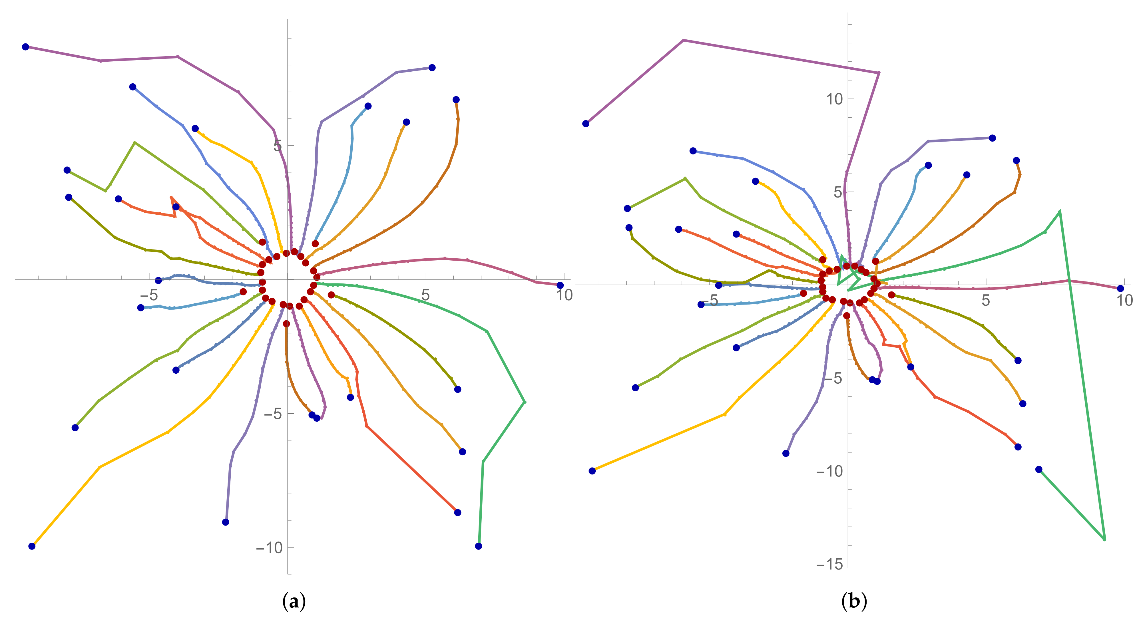
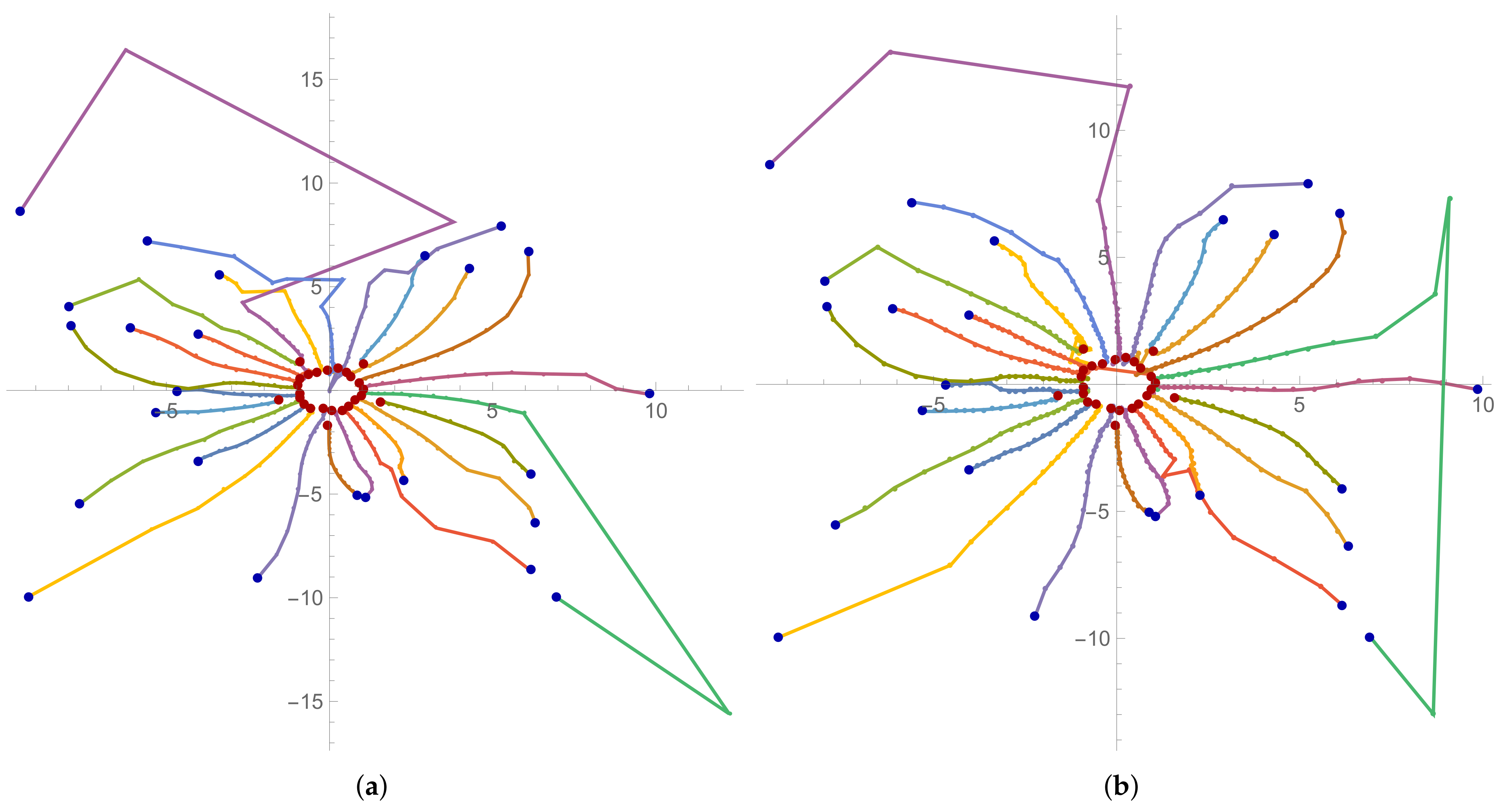
In the figures below, we present the trajectories of the approximations

$$x_1^{\left(j\right)},x_2^{\left(j\right)},\dots ,x_n^{\left(j\right)}\mathrm{for}j=0,1,\dots ,k$$

(95)

in the complex plane $\mathbb{C}$, where k is the smallest nonnegative integer that satisfies the stopping criterion (94). Besides, the roots of the polynomial f are presented with red points, and the initial approximations are presented with blue points.

We use CAS Wolfram Mathematica 12 to implement the corresponding algorithms and to present approximations of higher accuracy.

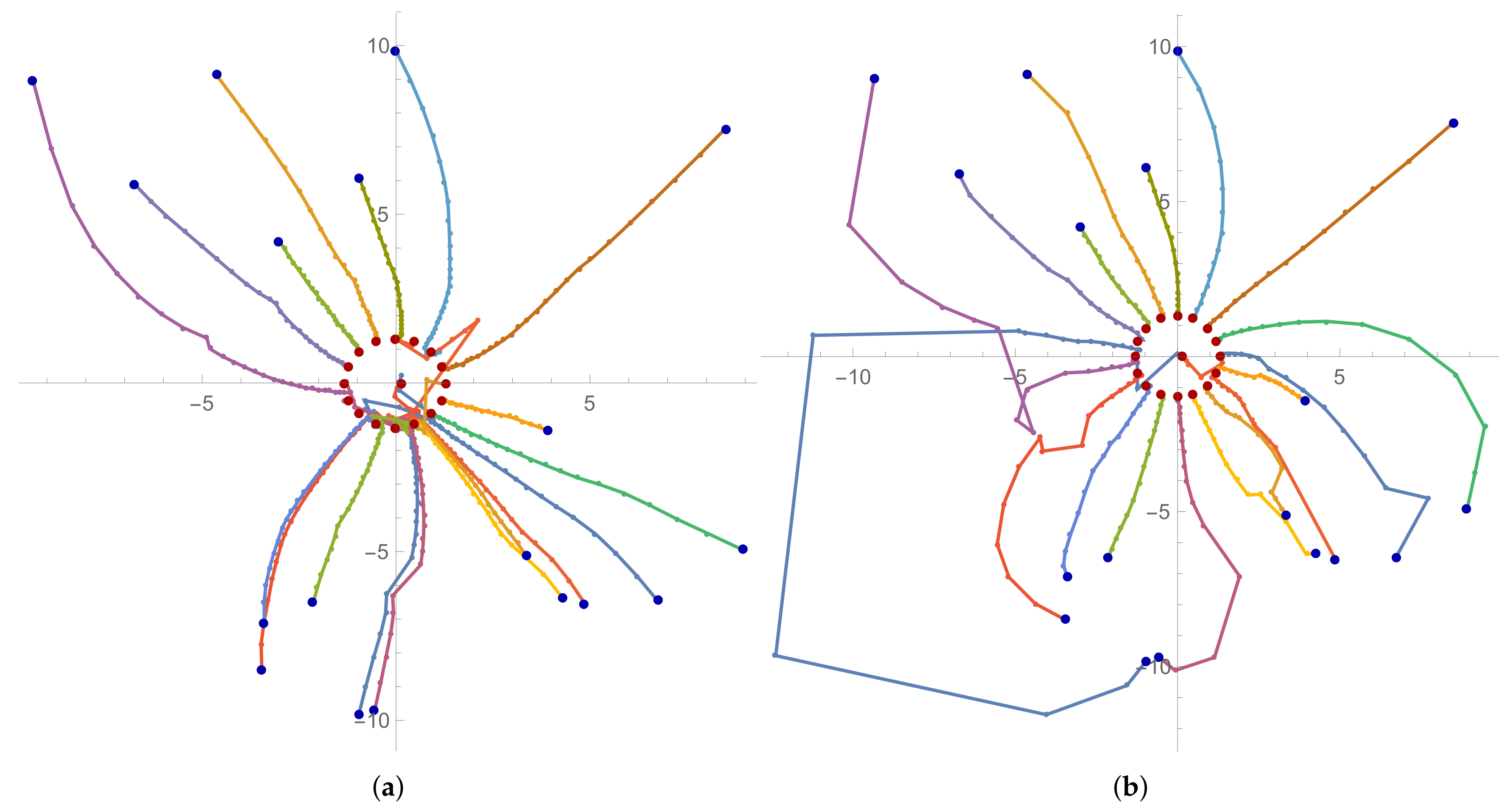
Example 1.

Let us consider Mignotte’s polynomial of the form $f\left(z\right)=z^n-{(az-1)}^2$$(n=18$, $a=9)$ ([28]), that is,

$$f_1\left(z\right)=z^{18}-81z^2+18z-1.$$

(96)

Our random initial approximation $x^{\left(0\right)}$ for this example is

$$\begin{array}{ccc}\hfill x^{\left(0\right)}& =& (-0.957-9.811i,-4.633+9.132i,-3.011+4.209i,4.862-6.533i,-6.742+5.896i,8.480+7.530i,\hfill \\ & & -0.011+9.864i,4.273-6.344i,-9.354+8.934i,-0.947+6.086i,-3.462-8.488i,-3.398-7.098i,\hfill \\ & & 3.901-1.402i,-0.552-9.705i,8.917-4.936i,6.740-6.454i,3.350-5.097i,-2.133-6.509i).\hfill \end{array}$$

In

Table 2. Numerical results for Example 1.

Method	r	s	${\mathit{E}}_{\mathit{f}}\left({\mathit{x}}^{\left(\mathit{s}\right)}\right)$	R	$\mathit{B}\left(\mathit{h}\left({\mathit{E}}_{\mathit{f}}\left({\mathit{x}}^{\left(\mathit{s}\right)}\right)\right)\right)$	${\mathit{\epsilon }}_{\mathit{s}}$	k	${\mathit{\epsilon }}_{\mathit{k}}$	${\mathit{\epsilon }}_{\mathit{k}+1}$
EW	4	51	$8.332\times {10}^{-6}$	0.038	$0.999$	$4.780\times {10}^{-15}$	52	$2.763\times {10}^{-30}$	$3.085\times {10}^{-91}$
EN	4	34	$1.247\times {10}^{-5}$	0.027	$0.999$	$7.156\times {10}^{-15}$	35	$1.388\times {10}^{-29}$	$1.968\times {10}^{-88}$
EE	5	28	$9.781\times {10}^{-3}$	0.038	$0.954$	$6.706\times {10}^{-12}$	29	$4.992\times {10}^{-20}$	$2.864\times {10}^{-60}$
EH	5	36	$1.069\times {10}^{-2}$	0.025	$0.967$	$7.420\times {10}^{-12}$	37	$1.432\times {10}^{-17}$	$4.466\times {10}^{-40}$

, we present the numerical results for Example 1. For instance, for Ehrlich’s method with Newton’s correction (EN) it is seen that the convergence criterion (93) is satisfied for $s=34$ and that the stopping criterion (94) is satisfied for $k=35$. Besides, at the 35th iteration each of the roots of the polynomial (96) is calculated with a guaranteed accuracy of $1.388\times {10}^{-29}$ and at 36th iteration the zeros of f are calculated with an accuracy of $1.968\times {10}^{-88}$.

In Figure 1 are presented the trajectories of the approximations (95) for the EW and EN methods for Example 1. The trajectories of the approximations (95) for the EE and EH methods for Example 1 are presented in Figure 2. Interesting trajectories can be seen. Some of them go a long way, others a shorter one, but each of them finds exactly one root of the polynomial.

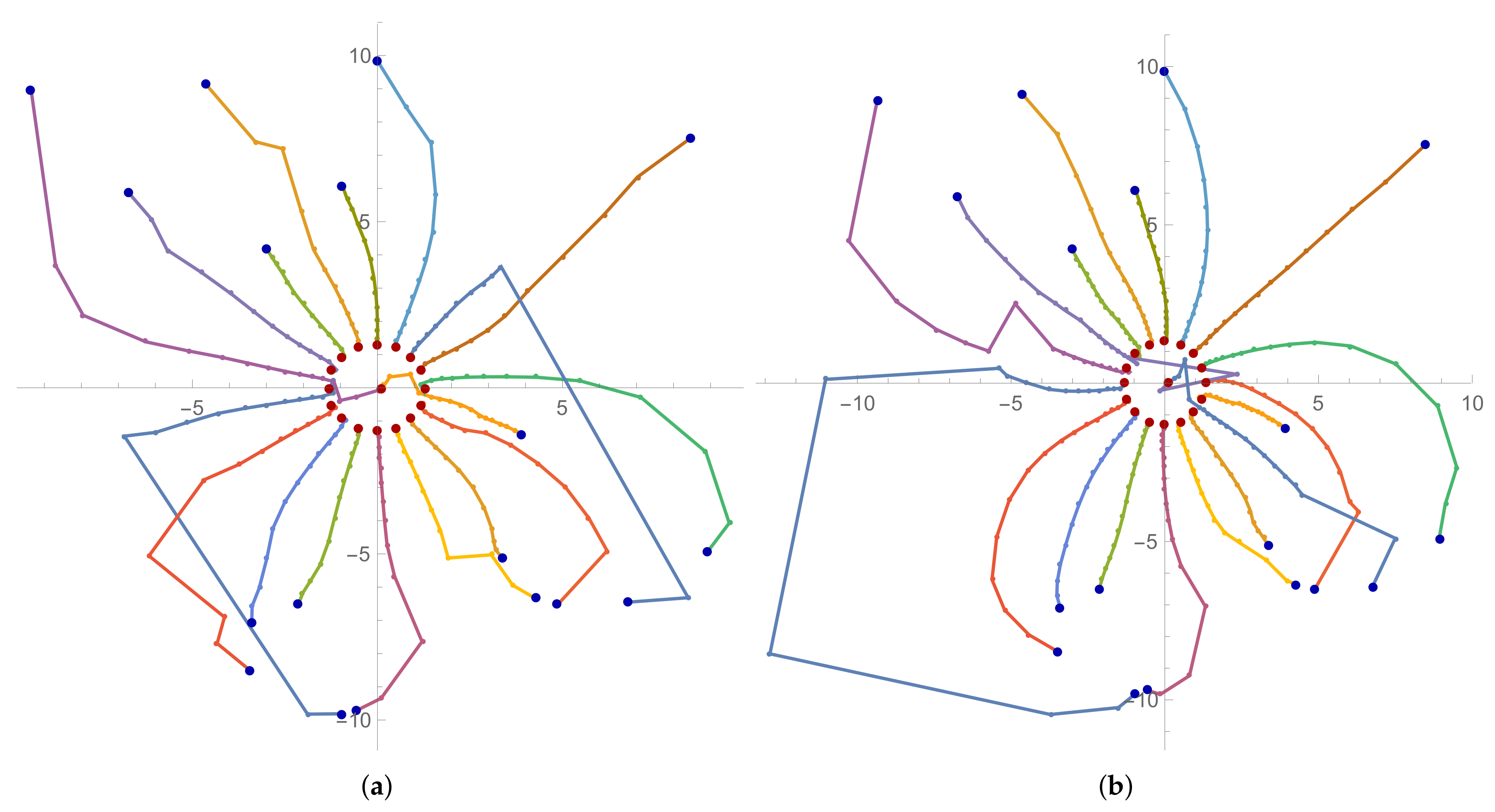
Example 2.

Following [6], we consider the following polynomial with random-integer coefficients from the interval $[1,8]$ and with the randomly chosen signs: -4.6cm0cm

$$\begin{array}{ccc}\hfill f_2\left(z\right)& =& z^{23}-5z^{22}+5z^{21}-6z^{20}+2z^{19}-8z^{18}+7z^{17}+6z^{16}-7z^{15}-6z^{14}+8z^{13}-6z^{12}\hfill \\ & & -4z^{11}-5z^{10}+5z^9+4z^8-6z^7+7z^6+3z^5-8z^4+5z^3-3z^2+7z-4.\hfill \end{array}$$

(97)

Our random initial approximation $x^{\left(0\right)}$ for Example 2 is -4.6cm0cm

$$\begin{array}{ccc}\hfill x^{\left(0\right)}& =& (2.752+6.162i,6.278+3.251i,3.498+1.819i,1.825+9.737i,0.777+7.693i,-0.116-4.020i,\hfill \\ & & -7.951+0.518i,9.455-5.858i,-6.789-0.057i,-8.564-1.775i,8.110-2.093i,8.198+4.769i,\hfill \\ & & -6.297+3.673i,5.917+9.915i,-6.838-0.181i,2.103+8.914i,2.098-3.961i,-9.998+3.813i,\hfill \\ & & 4.968-9.729i,-4.391-9.340i,-5.657-5.230i,7.303-6.733i,6.000+1.286i).\hfill \end{array}$$

Table 3. Numerical results for Example 2.

Method	r	s	${\mathit{E}}_{\mathit{f}}\left({\mathit{x}}^{\left(\mathit{s}\right)}\right)$	R	$\mathit{B}\left(\mathit{h}\left({\mathit{E}}_{\mathit{f}}\left({\mathit{x}}^{\left(\mathit{s}\right)}\right)\right)\right)$	${\mathit{\epsilon }}_{\mathit{s}}$	k	${\mathit{\epsilon }}_{\mathit{k}}$	${\mathit{\epsilon }}_{\mathit{k}+1}$
EW	4	43	$9.101\times {10}^{-4}$	0.030	$0.996$	$2.736\times {10}^{-4}$	44	$7.345\times {10}^{-20}$	$1.203\times {10}^{-85}$
EN	4	24	$2.231\times {10}^{-3}$	0.021	$0.990$	$4.122\times {10}^{-4}$	26	$1.344\times {10}^{-58}$	$3.145\times {10}^{-235}$
EE	5	21	$1.471\times {10}^{-6}$	0.030	$0.999$	$3.368\times {10}^{-7}$	22	$6.392\times {10}^{-35}$	$1.574\times {10}^{-173}$
EH	5	26	$3.222\times {10}^{-7}$	0.018	$0.999$	$5.654\times {10}^{-8}$	27	$2.806\times {10}^{-28}$	$1.826\times {10}^{-109}$

presents numerical results for Example 2. For instance, for Ehrlich’s method with Weierstrass’ correction (EW) it can be seen that the convergence criterion (93) is satisfied for $s=43$ and that the accuracy criterion (94) is satisfied for $k=44$. In addition, at 45th iteration each of the roots of the polynomial is calculated with a guaranteed accuracy of $1.203\times {10}^{-85}$.

In Figure 3 and Figure 4, one can see the trajectories (95) of the approximations of the EW, EN, EE and EH methods for Example 2. For instance, in Figure 3a we can see trajectories of the approximations of the EW method for the first 44 iterations $(k=44)$. Here we observe an interesting phenomenon: one of the trajectories goes in the opposite direction of the roots and after moving away quite far it changes its direction by moving horizontally, then it goes in the opposite direction of the roots again, but finally it turns back and finds its root.

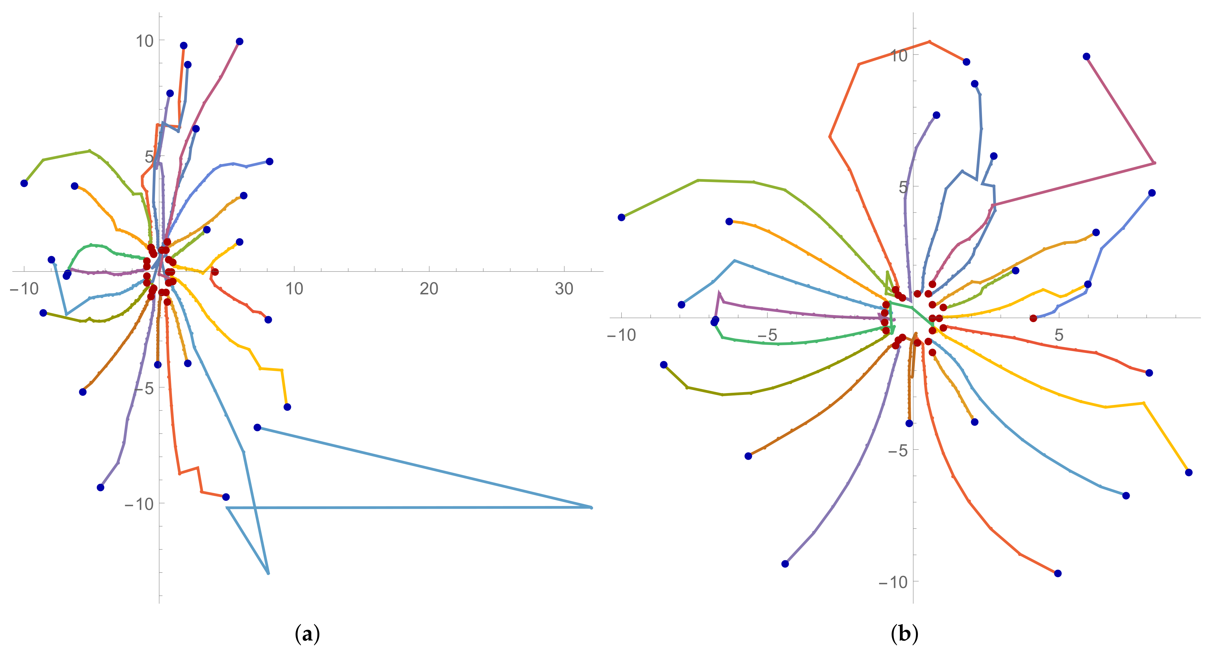
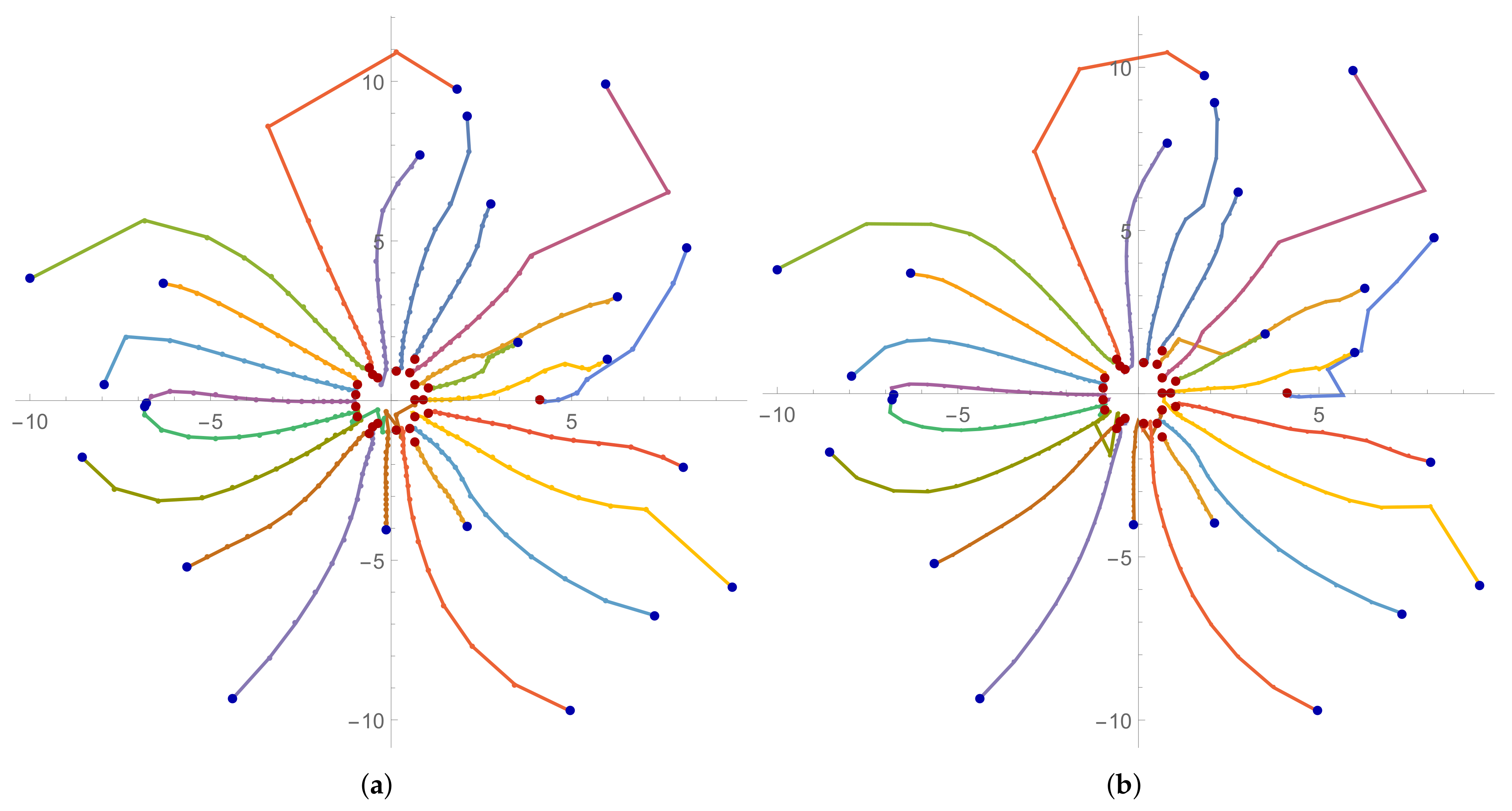
Example 3.

In this example, we consider the following polynomial with complex coefficients ([6]):

$$f_3\left(z\right)=z^{25}+(1+12i)z^{20}+(1-12i)z^{15}+(2+5I)z^{10}+(2-5i)z^5+10.$$

(98)

Our random initial approximation $x^{\left(0\right)}$ for Example 3 is -4.6cm0cm

$$\begin{array}{ccc}\hfill x^{\left(0\right)}& =& (-4.679-0.011i,6.315-6.406i,-7.688-5.513i,-6.122+3.004i,-2.216-9.083i,\hfill \\ & & 6.081+6.692i,2.904+6.444i,-3.343+5.607i,-9.449+8.689i,-7.895+3.077i,\hfill \\ & & 6.141-8.669i,-5.587+7.182i,2.297-4.381i,9.833-0.198i,6.923-9.948i,\hfill \\ & & -4.043-3.375i,4.288+5.872i,-7.983+4.070i,-4.055+2.701i,5.253+7.911i,\hfill \\ & & 0.871-5.063i,-5.296-1.060i,-9.234-9.964i,1.086-5.176i,6.147-4.075i).\hfill \end{array}$$

The numerical results for Example 3 are given in

Table 4. Numerical results for Example 3.

Method	r	s	${\mathit{E}}_{\mathit{f}}\left({\mathit{x}}^{\left(\mathit{s}\right)}\right)$	R	$\mathit{B}\left(\mathit{h}\left({\mathit{E}}_{\mathit{f}}\left({\mathit{x}}^{\left(\mathit{s}\right)}\right)\right)\right)$	${\mathit{\epsilon }}_{\mathit{s}}$	k	${\mathit{\epsilon }}_{\mathit{k}}$	${\mathit{\epsilon }}_{\mathit{k}+1}$
EW	4	22	$7.609\times {10}^{-4}$	0.028	$0.996$	$2.190\times {10}^{-4}$	24	$9.336\times {10}^{-53}$	$2.430\times {10}^{-207}$
EN	4	26	$2.078\times {10}^{-3}$	0.020	$0.991$	$6.135\times {10}^{-4}$	28	$3.866\times {10}^{-44}$	$2.217\times {10}^{-172}$
EE	5	21	$2.433\times {10}^{-2}$	0.028	$0.483$	$1.849\times {10}^{-2}$	23	$5.673\times {10}^{-44}$	$3.506\times {10}^{-215}$
EH	5	29	$1.187\times {10}^{-9}$	0.017	$0.999$	$3.333\times {10}^{-10}$	30	$3.635\times {10}^{-37}$	$6.418\times {10}^{-145}$

. For instance, for Ehrlich’s method with Halley’s correction (EH) it is seen that the convergence criterion (93) is satisfied for $s=29$ and that the stopping criterion (94) is satisfied for $k=30$, which means that the preset accuracy ${10}^{-15}$ is reached at 30th iteration. Moreover, the table shows that, at 30th iteration it is guarantees an accuracy of $3.635\times {10}^{-37}$ and at 31th iteration, it guarantees that each of the roots of the polynomial is calculated with a guaranteed accuracy of $6.418\times {10}^{-145}$.

In Figure 5 and Figure 6, one can see the trajectories (95) of the approximations of the EW, EN, EE and EH methods for Example 3. We again observe extremely interesting and strange trajectories.

It can be seen from Table 2, Table 3 and Table 4 that, in all experiments, Theorem 6 guarantees that each of the considered iterative methods of the family (5) is convergent under the given very rough initial approximation. In addition, we see on which iteration the preset accuracy is reached. Let us pay attention to the interesting fact that in each example Ehrlich’s method with Ehrlich’s correction (EE) needs the least iterations to satisfy convergence and accuracy criteria.

One can see from Figure 1, Figure 2, Figure 3, Figure 4, Figure 5 and Figure 6 that some initial points during iterating are not going to the nearest zero. Moreover, for the same polynomial and same initial approximation for different methods, some initial points during iterating go to a different zero of the polynomial.

11. Conclusions

In this paper, we construct and study the convergence of a new family of iterative methods for finding simultaneously all zeros of a polynomial. The new family is constructed by combining the classical Ehrlich’s iteration function and an arbitrary iteration function $\Phi$. Such methods are known as simultaneous methods with correction. In the literature, there are many simultaneous methods with particular corrections, but as far as the authors know, there are only two works [14,15] that study the convergence of some simultaneous method with arbitrary correction function.

We have proved several local and semilocal convergence theorems for Ehrlich’s method with a correction for a large class of iteration functions $\Phi$ under different initial conditions. The initial conditions of our semilocal convergence result are computationally verifiable, which is of practical importance. Our results generalize some results of Proinov [2], Proinov and Vasileva [9,25] and others. In Section 10, we present several numerical experiments that show the applicability of our semilocal convergence theorem.