Article

Time-Consistency of an Imputation in a Cooperative Hybrid Differential Game

Faculty of Applied Mathematics and Control Processes, St. Petersburg State University, 199034 St. Petersburg, Russia
*
Author to whom correspondence should be addressed.
Mathematics 2021, 9(15), 1830; https://doi.org/10.3390/math9151830
Submission received: 7 July 2021 / Revised: 26 July 2021 / Accepted: 31 July 2021 / Published: 3 August 2021

Abstract

:
This work is aimed at studying the problem of maintaining the sustainability of a cooperative solution in an n-person hybrid differential game. Specifically, we consider a differential game whose payoff function is discounted with a discounting function that changes its structure with time. We solve the problem of time-inconsistency of the cooperative solution using a so-called imputation distribution procedure, which was adjusted for this general class of differential games. The obtained results are illustrated with a specific example of a differential game with random duration and a hybrid cumulative distribution function (CDF). We completely solved the presented example to demonstrate the application of the developed scheme in detail. All results were obtained in analytical form and illustrated by numerical simulations.

1. Introduction

This contribution aims at bringing together two different concepts: the notion of sustainable cooperation from game theory and the notion of hybrid optimal control from the theory of hybrid systems. We first give a brief overview of the related results.
The concept of sustainable cooperation constitutes one of the central ingredients of cooperative game theory. Indeed, in many works it has been shown that a cooperative agreement may turn out to be unstable in the sense that the players may decide to break up the agreement at some intermediate time instant. To overcome this problem, Petrosyan, in [1], introduced the imputation distribution procedure (IDP) that has proven to be a very useful tool in the field of cooperative games. In the original paper [1], a fixed and finite-duration differential game was considered. Later, in [2], the notion of the IDP was extended to the class of differential games with infinite duration and a discounting function of a rather general form. Since then, there have been a number of papers devoted to the analysis of optimal problems with different types of discounting functions and their extension to the class of differential games (see, e.g., [3,4,5], where this problem was considered in both deterministic and stochastic settings, and [6] for the very recent results.)
Although the class of hybrid control systems was introduced more than 20 years ago, most results on hybrid control were formulated within the control-related framework and did not address the game-theoretic problems. We will be mostly interested in the hybrid optimal control, the direction that was actively developed during the first decade of the 21st century. We mention the works [7,8] for an overview of the main results on the hybrid optimal control. Some more examples of optimal control and—to some extent—differential games with regime switching can be found in [9,10,11,12,13]. It was only recently that the theory of hybrid control was formally extended to game-theoretic problems. The first attempt was made in [14]; later, in [15], a special but rather general class of hybrid differential games was considered in detail.
In this paper, we consider the problem of the sustainability of a cooperative solution in an n-person hybrid differential game. Earlier, a differential game with a random time horizon and discontinuous distribution was studied in [16], where only one jump was considered, and in [17], where the method of parametrization for calculation of the optimal controls was used. In this work we extend and generalize the results of [17] and put them in the context of hybrid optimal control.
To solve the formulated hybrid optimal control problem we use the method of parametrization, which is a well-known approach for numerical solution of optimal control problems, see, e.g., [18], but is relatively rarely used in the context of differential games. See [15] for some suggestions on how to apply this method to differential games with a switching structure. In short, the whole optimal control problem is decomposed into a number of subproblems, whose initial or final states are parametrized by some variables. These problems are solved backwards by applying the Pontryagin maximum principle [19] to each interval. If the respective optimal control problems admit analytical solutions, these solutions can be further used to determine the optimal values of switching states.
The described approach was successfully applied to a particular differential game with random duration and a composite cumulative distribution function. We computed the optimal controls and cooperative solutions, and determined the imputation distribution procedure.
This paper is organized in the following way. In Section 2 we present the formulation of the problem and formally state all necessary results. In particular, we present a uniform description of the hybrid discounting function using the notion of the hybrid hazard rate and give an explicit formula for computing the IDP. In Section 3 we work out a particular numeric example aimed at illustrating the previously formulated theoretic results. The last Section of the paper presents a conclusion.

2. Problem Formulation

2.1. Differential Game

Consider a differential game involving n participants (players): Γ d ( t 0 , x 0 ) (where the superscript d refers to discounting). Suppose the set of players is N = { 1 , , n } . Assume that the game initiates at the moment t 0 with the initial state x 0 .
The n-person differential game with prescribed duration T t 0 in which the integral payoff of the player i can be represented in the following form.
  • The dynamic constraint conditions for the game are given by
    x ˙ = g ( x ( t ) , u 1 ( t ) , . . . , u n ( t ) ) , x R h , x ( t 0 ) = x 0 . ,
    where (1) satisfy the standard requirements of existence and uniqueness. In particular, we assume that the function g ( x ( t ) , u 1 ( t ) , , u n ( t ) ) in (1) is continuously differentiable w.r.t. all its arguments;
  • The controls u i ( t ) are assumed to be piecewise continuous functions on the interval [ t 0 , T ] that belong to the set of admissible control values U i , which are consequently convex compact subsets of R k . The optimal controls are further assumed to be open-loop, i.e., they are defined as functions of t.
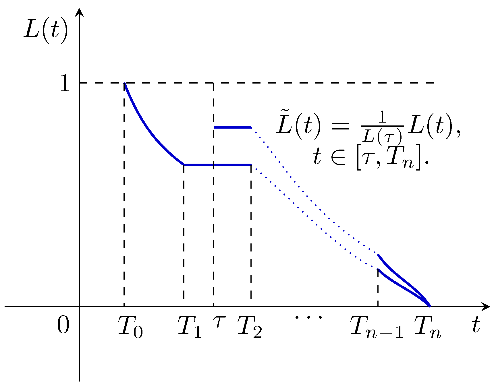
We will consider a differential game such that the payoff function changes its structure at specific time instants. Specifically, we will consider the situation in which the discounting function changes as one goes from one interval to another. Let σ = { T 0 , , T j , , T r } s.t. t 0 = T 0 < T 1 < < T r 1 < T r = T be an ordered sequence of time instants at which the switches occur. Then the payoff of player i is defined as follows:
K i ( x 0 , σ , u ) = j = 0 r 1 T j T j + 1 h i ( x ( t ) , u ( t ) ) L j ( t ) d t , T 0 = t 0 , T r = T ,
where L j ( t ) is the discounting function on the time interval t [ T j ; T j + 1 ) , and h i is the instantaneous payoff of the ith player. For the further analysis of problems with heterogeneous discounting see [3].
We assume the following conditions to be fulfilled for L j ( t ) , j = 0 , r 1 :
  • L 0 ( T 0 ) = 1 and L r 1 ( T ) = 0 , i.e., the discounting function is equal to 1 at the initial time and 0 at the final time;
  • L j ( t ) , j = 0 , , r 1 are non-increasing and continuously differentiable a.e. functions on [ T j ; T j + 1 ] ;
  • The discounting functions on the neighboring intervals agree at the switching points:
    L j ( T j + 1 ) = L j + 1 ( T j + 1 ) , j = 0 , r 2 .
An example of a discounting function is given in Figure 1. Note that this Figure contains not only the discounting function for the whole game, but also its restriction to a subgame as described in Section 2.2.
First, we present an approach to construct a composite discounting function for a given set of not necessarily coordinated functions. Let a set of functions l j ( t ) = 1 ϕ j ( t ) , j = 0 , , r 1 be given, where the functions ϕ j ( t ) satisfy the following conditions:
  • ϕ 0 ( T ) = 0 ; ϕ r 1 ( T ) = 1 ;
  • ϕ j ( t ) , j = 0 , , r 1 are non-decreasing and continuously differentiable a.e. on [ T j ; T j + 1 ] .
We have chosen to use this specific form of individual discounting functions expressed in terms of ϕ j to ensure that our presentation will be compatible with the subsequent exposition. However, this choice is merely a convention and can be changed as long as the individual discounting functions satisfy the required properties.
We define a composite discounting function L ( t ) on the base of the individual functions l j ( t ) = 1 ϕ j ( t ) , j = 0 , , r 1 while ensuring the property (3):
L ( t ) = L 0 ( t ) = l 0 ( t ) = 1 ϕ 0 ( t ) , t [ T 0 , T 1 ) , L 1 ( t ) = l 1 ( t ) L 0 ( T 1 ) l 1 ( T 1 ) = ( 1 ϕ 1 ( t ) ) L 0 ( T 1 ) 1 ϕ 1 ( T 1 ) , t [ T 1 , T 2 ) , L r 1 ( t ) = l r 1 ( t ) L r 2 ( T r 1 ) l r 1 ( T r 1 ) = ( 1 ϕ r 1 ( t ) ) L r 2 ( T r 1 ) 1 ϕ r 1 ( T r 1 ) , t [ T r 1 , T ] ,
We have previously assumed that ϕ j ( t ) exists a.e. for any j = 0 , , r 1 and t [ t 0 , T ] . Let us define the new function λ σ ( t ) , which is referred to as hazard rate in the reliability theory (see, e.g., [20]):
λ σ ( t ) = λ 0 ( t ) = ϕ 0 ( t ) 1 ϕ 0 ( t ) , t [ T 0 , T 1 ) , λ 1 ( t ) = ϕ 1 ( t ) 1 ϕ 1 ( t ) , t [ T 1 , T 2 ) , λ r 1 ( t ) = ϕ r 1 ( t ) 1 ϕ r 1 ( t ) , t [ T r 1 , T ] .
Let us consider the first interval [ T 0 ; T 1 ) and the hazard function λ 0 ( t ) . Then we have
λ 0 ( t ) = ϕ 0 ( t ) 1 ϕ 0 ( t ) = d d t ( 1 ϕ 0 ( t ) ) 1 ϕ 0 ( t ) = d d t l n ( 1 ϕ 0 ( t ) ) .
By integrating both sides of (6) from T 0 to t we obtain:
T 0 t λ 0 ( τ ) d τ = l n 1 ϕ 0 ( t ) 1 ϕ 0 ( T 0 ) ,
whence
e T 0 t λ 0 ( τ ) d τ = 1 ϕ 0 ( t ) 1 ϕ 0 ( T 0 ) , t [ T 0 , T 1 ) .
Finally, we can express 1 ϕ 0 ( t ) from (7) as
1 ϕ 0 ( t ) = ( 1 ϕ 0 ( T 0 ) ) e T 0 t λ 0 ( τ ) d τ = e T 0 t λ 0 ( τ ) d τ , t [ T 0 , T 1 ) ,
and the first component of the payoff function now can be represented as
T 0 T 1 h i ( x ( t ) , u ( t ) ) ( 1 ϕ 0 ( t ) ) d t = T 0 T 1 h i ( x ( t ) , u ( t ) ) e T 0 t λ 0 ( τ ) d τ d t .
Similarly to (6)–(8) we obtain the general formula
1 ϕ j ( t ) = ( 1 ϕ j ( T j ) ) e T j t λ j ( τ ) d τ , t [ T j , T j + 1 ) ) .
Substituting (9) into (5) we obtain an exponential representation for the composite discounting function L ( t ) :
L ( t ) = L 0 ( t ) = e T 0 t λ 0 ( τ ) d τ , t [ T 0 , T 1 ) , L 1 ( t ) = e T 0 T 1 λ 0 ( τ ) d τ · e T 1 t λ 1 ( τ ) d τ , t [ T 1 , T 2 ) , L r 1 ( t ) = j = 0 r 2 e T j T j + 1 λ j ( τ ) d τ · e T r 1 t λ r 1 ( τ ) d τ , t [ T r 1 , T ] ,
Note that while λ r 1 ( t ) is undefined at t = T , it can be shown that lim t T L ( t ) = 0 .
Thus we formulate the following result.
Proposition 1.
The payoff of the player i on the interval [ T j , T j + 1 ) , j = 0 , r 1 can be represented in the following form:
T j T j + 1 h i ( x ( t ) , u ( t ) ) L j ( t ) d t = e T 0 T 1 λ 0 ( τ ) d τ · e T 1 T 2 λ 1 ( τ ) d τ · e T j 1 T j λ j 1 ( τ ) d τ T j T j + 1 h i ( x ( t ) , u ( t ) ) e T j t λ j ( τ ) d τ d t ,
and the payoff of the player i at the whole game (12) can be written as
K i ( x 0 , σ , u ) = j = 0 r 1 k = 0 j 1 e T k T k + 1 λ k ( τ ) d τ · T j T j + 1 h i ( x ( t ) , u ( t ) ) e T j t λ j ( τ ) d τ d t , T 0 = t 0 , T r = T .
Thus the problem was reduced to the problem with different discounting factors λ j ( t ) on the different time intervals [ T j , T j + 1 ) (cf. [6]).
Taking (10) into account we can also rewrite the payoff of player i (12) in a more concise way:
K i ( x 0 , σ , u ) = T 0 T h i ( x ( t ) , u ( t ) ) L ( t ) d t .

2.2. Subgame

Let the game evolve and follow the trajectory x ( t ) . At any instantaneous time instant τ the players enter into a subgame Γ d ( τ , x ( τ ) ) , which is considered to be a new game from the position x ( τ ) with duration T τ .
To this end, we have to redefine the payoff function of the player i (13) to the payoff in a subgame. First we take into account that the discounting function L ˜ ( t ) for the game (which is a subgame) on time interval [ τ ; T ] should be normalized such that L ˜ ( τ ) = 1 , L ˜ ( T ) = 0 (see Figure 1).
Let the subgame start at τ [ T 0 , T ] . We define
L ˜ ( t ) = L ( t ) L ( τ ) .
Let τ [ T j ; T j + 1 ] , j = 0 , , r 1 , then for t [ τ ; T j + 1 ] we have
L j ( t ) L j ( τ ) = e T j t λ j ( τ ) d τ · e T j τ λ j ( τ ) d τ ,
and for the reason that t τ we have
L j ( t ) L j ( τ ) = e τ t λ j ( τ ) d τ .
Respectively, the discounting function in the whole subgame is defined as
L ˜ ( t ) = e τ t λ j ( τ ) d τ , t [ τ , T j + 1 ) , e τ T j λ j ( τ ) d τ · e T j t λ j ( τ ) d τ , t [ T j + 1 , T j + 2 ) , e τ T j λ j ( τ ) d τ · e T j T j + 1 λ j ( τ ) d τ · e T r 1 t λ r 1 ( τ ) d τ , t [ T r 1 , T ] .
We have the following form of the payoff of the player i in the subgame started at τ :
K i ( x ( τ ) , τ , σ j , u ) = τ T h i ( x ( t ) , u ( t ) ) L ˜ ( t ) d t = 1 L ( τ ) τ T h i ( x ( t ) , u ( t ) ) L ( t ) d t ,
where we used the notation σ j = σ { T 0 , , T j 1 } .
Now we obtain:
K i ( x 0 , T 0 , σ , u ) = T 0 T h i ( x ( t ) , u ( t ) ) L ( t ) d t = T 0 τ h i ( x ( t ) , u ( t ) ) L ( t ) d t + L ( τ ) · 1 L ( τ ) τ T h i ( x ( t ) , u ( t ) ) L ( t ) d t = T 0 τ h i ( x ( t ) , u ( t ) ) L ( t ) d t + L ( τ ) K i ( x ( τ ) , τ , σ j , u ) .

2.3. Cooperative Differential Game

Suppose that the game is played in a cooperative circumstance. In general, cooperation means that a group of participants agrees to cooperate in a form of coalition before starting the game.
Assume that all players agreed to maximize their total payoff, which we denote by V ( N , x 0 , σ ) . Let u ( t ) = { u 1 ( t ) , , u n ( t ) } be the optimal control, s.t.
( u 1 , . . . , u n ) = arg max u U 1 × × U n i = 1 n K i ( x 0 , σ , u )
and the corresponding trajectory x ( t ) obtained from (1) is said to be the optimal trajectory.
We also have
i = 1 n K i ( x 0 , σ , u ) = V ( N , x 0 , σ ) .
As the standard in cooperative games, all players in the coalition unanimously agree on a distribution mechanism (cooperative agreement) to divide the total payoff V ( N , x 0 , σ ) . It is probable that the solution of the current game loses it optimality at some instant based on the cooperative solution that was initially chosen, which means that the time-consistency for cooperative solution is not guaranteed. Since we are investigating a dynamic setting, it is necessary to define and determine an imputation distribution procedure [21,22,23,24], which is supposed to be in accordance with the payoff form.
Beforehand, we basically recall the notion of imputation: in an n-players cooperative game, an imputation is a distribution ξ = ( ξ 1 , , ξ n ) among players such that the sum of its coordinates is equivalent to the maximal payoff of the grand coalition and the component ξ i distributed to the i-th player is not less than what the player would acquire through a sole game. To be specific, suppose the set of players is N and the characteristic function [24] of the game is v : 2 N R , then ξ is an imputation if ξ 1 + + ξ n = v ( N ) and ξ i v ( i ) for all i = 1 , , n . The first property called efficiency makes sure that the imputation is a distribution method for the total gain among all players [25].
We adopt the definition of an imputation distribution procedure (IDP) first introduced in [21] for differential games with prescribed duration.
Definition 1.
Given an imputation ξ = ( ξ 1 , , ξ n ) R + n , such that for all i = 1 , , n we have
ξ i = T 0 T β i ( t ) L ( t ) d t = j = 0 r 1 T j T j + 1 β i ( t ) L j ( t ) d t = j = 0 r 1 k = 0 j 1 e T k T k + 1 λ j ( τ ) d τ T j T j + 1 β i ( t ) e T j t λ j ( τ ) d τ d t ,
then the vector function β ( t ) = ( β 1 ( t ) , , β n ( t ) ) R + n is called an imputation distribution procedure (IDP) in the game Γ d ( t 0 , x 0 ) .
Furthermore, we define the notion of time-consistency of an imputation.
Definition 2.
An imputation ξ = ( ξ 1 , , ξ n ) R n in the game Γ d ( t 0 , x 0 ) is time-consistent if there exists an IDP β ( t ) = ( β 1 ( t ) , , β n ( t ) ) R N such that for any ϑ [ 0 , T ] the vector
ξ i ϑ = 1 L ( ϑ ) ϑ T β i ( t ) L ( t ) d t = ϑ T β i ( t ) L ˜ ( t ) d t
belongs to the same cooperative agreement in the subgame Γ d ( ϑ , x ) , i.e., ξ ϑ is an imputation in Γ d ( ϑ , x ) .
We now check the time consistency property in detail. Let ϑ [ T j ; T j + 1 ) . Then
ξ i ϑ = ϑ T j + 1 β i ( t ) e ϑ t λ k ( τ ) d τ d t + k = j + 1 r 1 T k T k + 1 β i ( t ) e ϑ T j + 1 λ k ( τ ) d τ l = j + 1 k 1 e T l T l + 1 λ l ( τ ) d τ e T k t λ k ( τ ) d τ d t .
Then we obtain
ξ i = k = 0 j 1 T k T k + 1 β i ( t ) L k ( t ) d t + T j ϑ β i ( t ) L j ( t ) d t + e T 0 T 1 λ 0 ( τ ) d τ · e T 1 T 2 λ 1 ( τ ) d τ · e T j ϑ λ j ( τ ) d τ ξ i ϑ .
By taking the derivative with respect to ϑ , ϑ [ T j ; T j + 1 ) and noting that ξ i is a constant, we obtain
β i ( ϑ ) L j ( ϑ ) + k = 0 j 1 e T k T k + 1 λ k ( τ ) d τ · e T j ϑ λ j ( τ ) d τ ( ξ i ϑ ) ϑ λ j ( ϑ ) k = 0 j 1 e T k T k + 1 λ k ( τ ) d τ · e T j ϑ λ j ( τ ) d τ ξ i ϑ = 0 .
Recall that L j ( ϑ ) = k = 0 j 1 e T k T k + 1 λ k ( τ ) d τ · e T j ϑ λ j ( τ ) d τ . Canceling the respective terms we obtain
β i ( ϑ ) + ( ξ i ϑ ) ϑ λ j ( ϑ ) ξ i ϑ = 0 ,
whence the final expression for β i ( ϑ ) results:
β i ( ϑ ) = λ j ( ϑ ) ξ i ϑ ( ξ i ϑ ) ϑ , ϑ [ T j ; T j + 1 ) , j = 0 , , r 1 .
We now formally state this result.
Theorem 1.
Let the imputation ξ i t of the game Γ d ( t , x ( t ) ) be an absolutely continuous function of t [ 0 , T ] . If the IDP has the form
β i ( ϑ ) = λ σ ( ϑ ) ξ i ϑ ( ξ i ϑ ) ϑ ,
for any ϑ [ 0 , T ] then ξ i is a time-consistent imputation in the game Γ d ( 0 , x 0 ) with IDP given by (16).
Note that this formula has the same form [2,24] as the IDP computed for a problem with a single discounting function with the only difference that instead of λ ( t ) we use the composite hazard rate function λ σ ( t ) . Furthermore, if we consider a game with a prescribed duration and without discounting, we have λ σ ( ϑ ) 0 , and (18) takes the standard form as, e.g., in [23].

3. Computation of IDP: A Numerical Example

3.1. Description of the Model

This Section will build upon the results presented in [17]. We will skip most results that were previously reported except for those that are necessary for the understanding of the current material.
Consider a model example describing the differential game of investment into the stock of knowledge. Assume that there are N individuals investing in a public stock of knowledge [26]. Let x ( t ) be the stock of knowledge at time t and u i ( t ) be the ith agent’s investment in public knowledge at time t. The dynamics of the stock of knowledge is described by
x ˙ ( t ) = i = 1 N u i ( t ) , x R , u i U R , x ( t 0 ) = x 0 .
If each agent derives linear utility from the consumption of knowledge, the instantaneous payoff of the ith player is described by
h i ( x ( t ) , u ( t ) ) = q i x ( t ) r i u i 2 ( t ) , q i > 0 , r i > 0 .
Further assume that the time instants are σ = { 0 , T ¯ δ , T ¯ + δ , T 1 , T 2 , T 3 } , where T ¯ > δ and T ¯ + δ < T 1 < T 2 < T 3 . We define the ϕ i ( t ) functions as follows:
ϕ k ( t ) = 0 , if k = 0 , t [ 0 , T ¯ δ ) , ( 1 p 1 p 2 ) t T ¯ + δ 2 δ , if k = 1 , t [ T ¯ δ , T ¯ + δ ) , 1 p 1 p 2 , if k = 2 , t [ T ¯ + δ , T 1 ) , 1 p 2 , if k = 3 , t [ T 1 , T 2 ) , 1 , if k = 4 , t [ T 2 , T 3 ] .
Note that the conditions formulated in Section 2 hold, i.e., ϕ 0 ( 0 ) = 0 , ϕ 4 ( T 3 ) = 1 , and all functions ϕ i ( τ ) are continuously differentiable.
This choice can be interpreted as a problem with random duration in which the game ends at the random time instant with a known cumulative distribution function (21). For instance, this c.d.f. means that the game cannot stop before T ¯ δ but then it may stop with the probability given by the uniform distribution at the time interval [ T ¯ δ ; T ¯ + δ ] . Let us denote this game as Γ r ( t 0 , x 0 ) , where the superscript r refers to random duration.

3.2. Optimal Solution

We consider the cooperative game. Assume that all players opt to cooperate and, hence, group their efforts to maximize the total payoff.
i = 1 n K i ( x 0 , σ , u ) max u
The optimization problem can be tackled using state parametrization under four continuous intervals (see [17] for details):
I 1 : [ 0 ; T ¯ δ ] both sides are fixed { x 0 , x 1 } I 2 : [ T ¯ δ ; T ¯ + δ ] both sides are fixed { x 1 , x 2 } I 3 : [ T ¯ + δ ; T 1 ] both sides are fixed { x 2 , x 3 } I 4 : [ T 1 ; T 2 ] only one side is fixed { x 3 }
Note that we do not consider the fifth interval [ T 2 , T 3 ] because on this interval ϕ 4 ( t ) = 0 and, respectively, l 4 ( t ) = 0 .
For the interval I 1 , we obtain the following expressions for the optimal trajectory and control:
x ( t ) I 1 = ( x 1 x 0 ) t ( T ¯ δ ) + 1 4 q ^ t ( T ¯ δ t ) i = 1 n 1 r i + x 0 , u i ( t ) I 1 = x 1 x 0 r i i = 1 n 1 r i ( T ¯ δ ) + q ^ ( T ¯ δ ) 4 r i q ^ t 2 r i .
For the interval I 2 , we have the expressions for the optimal trajectory and control shown below:
x ( t ) I 2 = q ^ i = 1 n 1 r i 2 ( 1 p 1 p 2 ) 2 δ 2 χ ( t ) 2 4 + + 2 ( x 2 x 1 ) ( 1 p 1 p 2 ) q ^ i = 1 n 1 r i δ 2 ( 1 + p 1 + p 2 ) 2 ln ( p 1 + p 2 ) ( 1 p 1 p 2 ) ln χ ( t ) 2 δ + x 1 , u i ( t ) I 2 = q ^ χ ( t ) 4 r i ( 1 p 1 p 2 ) 2 ( x 2 x 1 ) ( 1 p 1 p 2 ) q ^ δ 2 i = 1 n 1 r i ( 1 + p 1 + p 2 ) 2 r i i = 1 n 1 r i χ ( t ) ln ( p 1 + p 2 ) ,
where χ ( t ) = 2 δ ( 1 p 1 p 2 ) ( t T ¯ + δ ) .
For the interval I 3 , we obtain:
x ( t ) I 3 = i = 1 n 1 r i ( x 3 x 2 ) ( t T ¯ δ ) i = 1 n 1 r i ( T 1 T ¯ δ ) + q ^ ( T 1 T ¯ δ ) ( t T ¯ δ ) 4 q ^ ( t T ¯ δ ) 2 4 + x 2 , u i ( t ) I 3 = ( x 3 x 2 ) r i i = 1 n 1 r i ( T 1 T ¯ δ ) + q ^ ( T 1 + T ¯ + δ 2 t ) 4 r i .
For the interval I 4 , we have:
x ( t ) I 4 = q ^ i = 1 n 1 4 r i ( t T 1 ) ( t + T 1 2 T 2 ) + x 3 , u i ( t ) I 4 = q ^ ( T 2 t ) 2 r i .
The switching states x 1 , x 2 , x 3 are given below:
x 1 = q ^ ( T ¯ δ ) ( p 1 ( T 1 T ¯ ) + p 2 ( T 2 T ¯ ) + T ¯ + δ 2 ) i = 1 n 1 r i 2 + x 0 , x 2 = q ^ δ 2 i = 1 n 1 r i 2 ( 1 p 1 p 2 ) 2 ( ( p 1 + p 2 ) 2 ( 2 ln ( p 1 + p 2 ) 1 ) + 1 ) q ^ δ i = 1 n 1 r i ln ( p 1 + p 2 ) 1 p 1 p 2 ( p 1 ( T 1 T ¯ δ ) + p 2 ( T 2 T ¯ δ ) ) + x 1 , x 3 = i = 1 n 1 r i q ^ ( T 1 T ¯ δ ) 2 ( p 1 + p 2 ) ( p 1 + p 2 ) ( T 1 T ¯ δ ) 2 + p 2 ( T 2 T 1 ) + x 2 .
Note that all optimal values of the switching states depend (either directly or indirectly) on the initial state x 0 .

3.3. Optimal Solutions for Subgames

In this section we consider the optimal solutions in a subgame starting from some time ϑ [ 0 , T 3 ] . The formal definition of a subgame and the respective analysis of the related optimal control problems is presented in Section 2.2.
Subgame starting at ϑ [ T ¯ δ , T ¯ + δ ) : Consider a subgame Γ r ( ϑ , x ) such that ϑ [ T ¯ δ , T ¯ + δ ) . The conditional c.d.f., which corresponds to the function L ˜ ( t ) defined in Section 2.2, takes the following form:
F ϑ ( t ) = ϕ ( t ) ϕ ( ϑ ) 1 ϕ ( ϑ ) , t [ ϑ , T ¯ + δ ) 1 p 1 p 2 ϕ ( ϑ ) 1 ϕ ( ϑ ) , t [ T ¯ + δ , T 1 ) 1 p 2 ϕ ( ϑ ) 1 ϕ ( ϑ ) , t [ T 1 , T 2 ) , 1 , t T 2 .
The expected integral payoff for player i in this subgame is given by the following formula:
K i ( ϑ , x , u 1 , . . . , u n ) = 1 1 ϕ ( ϑ ) ϑ T ¯ + δ ( 1 ϕ ( t ) ) h i ( t ) d t + T ¯ + δ T 1 ( p 1 + p 2 ) h i ( t ) d t + T 1 T 2 p 2 h i ( t ) d t .
Subgame starting at ϑ [ T ¯ + δ , T 1 ] : Consider a subgame Γ r ( ϑ , x ) such that ϑ [ T ¯ + δ , T 1 ] . The conditional c.d.f. takes the following form:
F ϑ ( t ) = 0 , t [ ϑ , T 1 ) p 1 p 1 + p 2 , t [ T 1 , T 2 ) 1 , t T 2 .
The expected integral payoff for player i in this subgame is given by the following formula:
K i ( ϑ , x , u 1 , . . . , u n ) = 1 p 1 + p 2 ϑ T 1 ( p 1 + p 2 ) h i ( t ) d t + T 1 T 2 p 2 h i ( t ) d t .
Subgame starting at ϑ [ T 1 , T 2 ] : Consider a subgame Γ r ( ϑ , x ) such that ϑ [ T 1 , T 2 ] . The conditional c.d.f. takes the following form:
F ϑ ( t ) = 0 , t [ ϑ , T 2 ) 1 , t T 2 .
The expected integral payoff for player i in this subgame is indicated in the following formula:
K i ( ϑ , x , u 1 , . . . , u n ) = 1 p 2 ϑ T 2 p 2 h i ( t ) d t .
Finally, we reach the following general expression for the expected integral payoff of player i in the subgame Γ r ( ϑ , x ) , ϑ [ t 0 , T 2 ] :
K i ( ϑ , x , u 1 , . . . , u n ) = ϑ T ¯ δ h i ( τ ) d τ + T ¯ δ T ¯ + δ ( 1 ϕ ( τ ) ) h i ( τ ) d τ + T ¯ + δ T 1 ( p 1 + p 2 ) h i ( τ ) d τ + T 1 T 2 p 2 h i ( τ ) d τ , if   ϑ [ t 0 ; T ¯ δ ) ; 1 1 ϕ ( ϑ ) ϑ T ¯ + δ ( 1 ϕ ( t ) ) h i ( t ) d t + T ¯ + δ T 1 ( p 1 + p 2 ) h i ( t ) d t + T 1 T 2 p 2 h i ( t ) d t , if   ϑ [ T ¯ δ , T ¯ + δ ) ; 1 p 1 + p 2 ϑ ¯ T 1 ( p 1 + p 2 ) h i ( t ) d t + T 1 T 2 p 2 h i ( t ) d t , if   ϑ [ T ¯ + δ , T 1 ) ; 1 p 2 ϑ ¯ ¯ T 2 p 2 h i ( t ) d t , if   ϑ [ T 1 , T 2 ] .

3.4. Computation of the Imputation Distribution Procedure (IDP)

The definition of the imputation and the imputation distribution procedure were given in Section 2.3. Here we specify the previously given definitions for the considered differential game.
Specifically, we have that for a given imputation ξ = ( ξ 1 , , ξ n ) R + n in a game Γ r ( t 0 , x 0 ) , the imputation distribution procedure satisfies the following equation (compare to the equation in Definition 1):
ξ i = t 0 T ¯ δ β i ( τ ) d τ + T ¯ δ T ¯ + δ ( 1 ϕ ( τ ) ) β i ( τ ) d τ + T ¯ + δ T 1 ( p 1 + p 2 ) β i ( τ ) d τ + T 1 T 2 p 2 β i ( τ ) d τ .
The next Definition formalizes the property of time-consistency for imputations.
Definition 3.
An imputation ξ = ( ξ 1 , , ξ N ) R + N in a game Γ r ( t 0 , x ) is time-consistent if there exists an IDP β ( t ) = ( β 1 ( t ) , , β n ( t ) ) R + n such that:
  • For all ϑ [ t 0 , T ¯ δ ) the vector ξ ϑ = ( ξ 1 ϑ , , ξ n ϑ ) , where
    ξ i ϑ = ϑ T ¯ δ β i ( τ ) d τ + T ¯ δ T ¯ + δ ( 1 ϕ ( τ ) ) β i ( τ ) d τ + T ¯ + δ T 1 ( p 1 + p 2 ) β i ( τ ) d τ + T 1 T 2 p 2 β i ( τ ) d τ .
    for all i = 1 , , n , belongs to the same optimality principle in the subgame Γ r ( ϑ , x ) , i.e., ξ ϑ is an imputation in Γ r ( ϑ , x ) ;
  • For all ϑ [ T ¯ δ , T ¯ + δ ) the vector ξ ϑ = ( ξ 1 ϑ , , ξ n ϑ ) , where
    ξ i ϑ = 1 1 ϕ ( ϑ ) ϑ T ¯ + δ ( 1 ϕ ( t ) ) β i ( t ) d t + T ¯ + δ T 1 ( p 1 + p 2 ) β i ( t ) d t + T 1 T 2 p 2 β i ( t ) d t .
    for all i = 1 , , n , belongs to the same optimality principle in the subgame Γ r ( ϑ , x ) , i.e., ξ ϑ is an imputation in Γ r ( ϑ , x ) ;
  • For all ϑ [ T ¯ + δ , T 1 ] the vector ξ ϑ = ξ 1 ϑ , , ξ n ϑ , where
    ξ i ϑ = 1 p 1 + p 2 ϑ T 1 ( p 1 + p 2 ) β i ( t ) d t + T 1 T 2 p 2 β i ( t ) d t ,
    for all i = 1 , , n , belongs to the same optimality principle in the subgame Γ r ( ϑ , x ) , i.e., ξ ϑ is an imputation in Γ r ( ϑ , x ) ;
  • For all ϑ [ T 1 , T 2 ] the vector ξ ϑ = ξ 1 ϑ , , ξ n ϑ , where
    ξ i ϑ = 1 p 2 ϑ T 2 p 2 β i ( t ) d t ,
    for all i = 1 , , n , belongs to the same optimality principle in the subgame Γ r ( ϑ , x ) , i.e., ξ ϑ is an imputation in Γ r ( ϑ , x ) .
Following the analysis presented in Section 2.3, we formulate the following formulas for determining the IDP.
Proposition 2.
If ϑ [ t 0 , T ¯ δ ) , then for all i = 1 , , n , the i-th coordinate of the IDP is given by:
β i ( ϑ ) = ( ξ i ϑ ) .
If ϑ [ T ¯ δ , T ¯ + δ ) , then for all i = 1 , , n , the i-th coordinate of the IDP is given by:
β i ( ϑ ) = ( ϕ ( ϑ ) ) 1 ϕ ( ϑ ) ξ i ϑ ( ξ i ϑ ) .
If ϑ [ T ¯ + δ , T 1 ) , then for all i = 1 , , n , the i-th coordinate of the IDP is given by:
β i ( ϑ ) = ( ξ i ϑ ) .
If ϑ [ T 1 , T 2 ] , then for all i = 1 , , n , the i-th coordinate of the IDP is given by:
β i ( ϑ ) = ( ξ i ϑ ) .
We conclude this part with the following proposition.
Proposition 3.
The imputation { ξ i } given by (28) is time-consistent if the respective IDPs are defined according to (29)–(32).

3.5. Numerical Illustration of the Computed IDP Numeric Example

To illustrate the obtained results we will consider the same parameter set as in [17]:
n = 3 number of players x 0 = 20 initial number of funds t 0 = 0 initial time T ¯ = 10 , δ = 3 , T 1 = 70 , T 2 = 75 time structure parameters q 1 = 1 , q 2 = 3 , q 3 = 6 , values of coefficients of payoffs r 1 = 20 , r 2 = 1 , r 3 = 4 p 1 = 0.1 , p 2 = 0.2 probabilities to stop the investment at T 1 , T 2 .
Both the imputation and the imputation distribution procedure are illustrated in Figure 2. Note that the optimal solution undergoes a discontinuity at time t = T 1 , where the cumulative probability function is discontinuous as well. One can observe that the imputation distribution procedure is positive during the whole interval of time except a short period of time between t = 11 and t = 13 .
The resulting imputation and the imputation distribution function are computed in an egalitarian way in which the distribution for each player is taken in the form of the average of total payoff. Obviously, this approach can be extended to any further type of imputation.

4. Conclusions

The aim of this paper was not only to describe an approach of computing the IDP for a class of hybrid differential games, but also to present a worked-out example aimed at demonstrating the described procedure in full detail. The main points of the paper are as follows: (1) The differential game with hybrid discounting function can well describe a wide class of differential games, including the games with random horizon and a hybrid CDF; (2) the considered class of differential games can be described in a uniform way by using the notion of a hybrid hazard rate; (3) finally, it is possible to completely solve a problem of reasonable complexity. Our future work will be concentrated on extending the class of hybrid games.

Author Contributions

Conceptualization, E.G.; Formal analysis, A.Z.; Investigation, A.Z. and S.S.; Methodology, E.G.; Project administration, A.Z.; Supervision, E.G.; Validation, A.Z. and S.S.; Writing—original draft, A.Z., E.G. and S.S.; Writing—review and revising, E.G. All authors have read and consented to the published version of the manuscript.

Funding

The work by E. Gromova and A. Zaremba was supported by a grant from Russian Science Foundation, no. 17-11-01079.

Conflicts of Interest

The authors declare no conflict of interest.

References

  1. Petrosyan, L.; Murzov, N. Game-theoretic problems of mechanics. Litovsk. Math. Sb. 1966, 7, 423–433. [Google Scholar]
  2. Marin-Solano, J.; Shevkoplyas, E. Non-constant discounting and differential games with random time horizon. Automatica 2011, 47, 2626–2638. [Google Scholar] [CrossRef]
  3. Marin-Solano, J.; Patxot, C. Heterogeneous discounting in economic problems. Optim. Control Appl. Methods 2012, 33, 32–50. [Google Scholar] [CrossRef]
  4. de-Paz, A.; Marin-Solano, J.; Navas, J. A consumption investment problem with heterogeneous discounting. Math. Soc. Sci. 2013, 66, 221–232. [Google Scholar] [CrossRef]
  5. de-Paz, A.; Marin-Solano, J.; Navas, J.; Roch, O. Consumption, investment and life insurance strategies with heterogeneous discounting. Insur. Math. Econ. 2014, 54, 66–75. [Google Scholar] [CrossRef] [Green Version]
  6. de Frutos Cachorro, J.; Marin-Solano, J.; Navas, J. Competition between different groundwater uses under water scarcity. Water Resour. Econ. 2021, 33, 100173. [Google Scholar] [CrossRef]
  7. Riedinger, P.; Iung, C.; Kratz, F. An optimal control approach for hybrid systems. Eur. J. Control 2003, 9, 449–458. [Google Scholar] [CrossRef] [Green Version]
  8. Shaikh, M.S.; Caines, P.E. On the hybrid optimal control problem: Theory and algorithms. IEEE Trans. Autom. Control 2007, 52, 1587–1603. [Google Scholar] [CrossRef]
  9. Bonneuil, N.; Boucekkine, R. Optimal transition to renewable energy with threshold of irreversible pollution. Eur. J. Oper. Res. 2016, 248, 257–262. [Google Scholar] [CrossRef] [Green Version]
  10. Elliott, R.J.; Siu, T.K. A stochastic differential game for optimal investment of an insurer with regime switching. Quant. Financ. 2011, 11, 365–380. [Google Scholar] [CrossRef]
  11. Gromov, D.; Bondarev, A.; Gromova, E. On periodic solution to control problem with time-driven switching. Optim. Lett. 2021. in print. [Google Scholar] [CrossRef]
  12. Kuhn, M.; Wrzaczek, S. Rationally Risking Addiction: A Two-Stage Approach. In Dynamic Modeling and Econometrics in Economics and Finance; Dynamic Economic Problems with Regime Switches; Springer: Berlin/Heidelberg, Germany, 2021; pp. 85–110. [Google Scholar]
  13. Reddy, P.; Schumacher, J.; Engwerda, J. Optimal management with hybrid dynamics—The shallow lake problem. In Mathematical Control Theory I; Springer: Berlin/Heidelberg, Germany, 2015; pp. 111–136. [Google Scholar]
  14. Gromov, D.; Gromova, E. Differential games with random duration: A hybrid systems formulation. Contrib. Game Theory Manag. 2014, 7, 104–119. [Google Scholar]
  15. Gromov, D.; Gromova, E. On a Class of Hybrid Differential Games. Dyn. Games Appl. 2017, 7, 266–288. [Google Scholar] [CrossRef]
  16. Gromova, E.; Malakhova, A.; Palestini, A. Payoff Distribution in a Multi-Company Extraction Game with Uncertain Duration. Mathematics 2018, 6, 165. [Google Scholar] [CrossRef] [Green Version]
  17. Zaremba, A.; Gromova, E.; Tur, A. A Differential Game with Random Time Horizon and Discontinuous Distribution. Mathematics 2020, 8, 2185. [Google Scholar] [CrossRef]
  18. Lin, Q.; Ryan, L.; Kok, L.T. The control parameterization method for nonlinear optimal control: A survey. J. Ind. Manag. Optim. 2014, 10, 275–309. [Google Scholar] [CrossRef]
  19. Pontryagin, L.; Boltyanskii, V.; Gamkrelidze, R.; Mishchenko, E. The Mathematical Theory of Optimal Processes; Interscience: New York, NY, USA, 1962. [Google Scholar]
  20. Finkelstein, M. Failure Rate Modelling for Reliability and Risk; Springer: Berlin/Heidelberg, Germany, 2008; 290p. [Google Scholar]
  21. Petrosjan, L. Stability of solutions in differential many-player games. Vestn. Leningr. Univ. 1977, 4, 46–52. (In Russian) [Google Scholar]
  22. Petrosjan, L.A. The Shapley value for differential games. New Trends Dyn. Games Appl. 1995, 3, 409–417. [Google Scholar]
  23. Petrosyan, L.; Danilov, N. Cooperative Differential Games and Their Applications; Izd. Tomskogo Universiteta: Tomsk, Russia, 1982. [Google Scholar]
  24. Petrosyan, L.A.; Zaccour, G. Cooperative differential games with transferable payoffs. In Handbook of Dynamic Game Theory; Springer: Cham, Switzerland, 2018; pp. 595–632. [Google Scholar]
  25. Gromova, E. The Shapley value as a sustainable cooperative solution in differential games of three players. In Recent Advances in Game Theory and Applications; Birkhäuser: Cham, Switzerland, 2016; pp. 67–89. [Google Scholar]
  26. Dockner, E.J.; Jorgensen, S.; Van Long, N.; Sorger, G. Differential Games in Economics and Management Science; Cambridge University Press: Cambridge, UK, 2000. [Google Scholar]
Figure 1. Discounting function for a game and for the subgame starting at t = τ .
Mathematics 09 01830 g001
Figure 2. The imputation for the player (green) and the imputation distribution procedure (IDP) (blue).
Mathematics 09 01830 g002
Publisher’s Note: MDPI stays neutral with regard to jurisdictional claims in published maps and institutional affiliations.

