
Chaotic Path Planning for 3D Area Coverage Using a Pseudo-Random Bit Generator from a 1D Chaotic Map

 ,
, 
 ,
,  ,
, 
Abstract
:1. Introduction
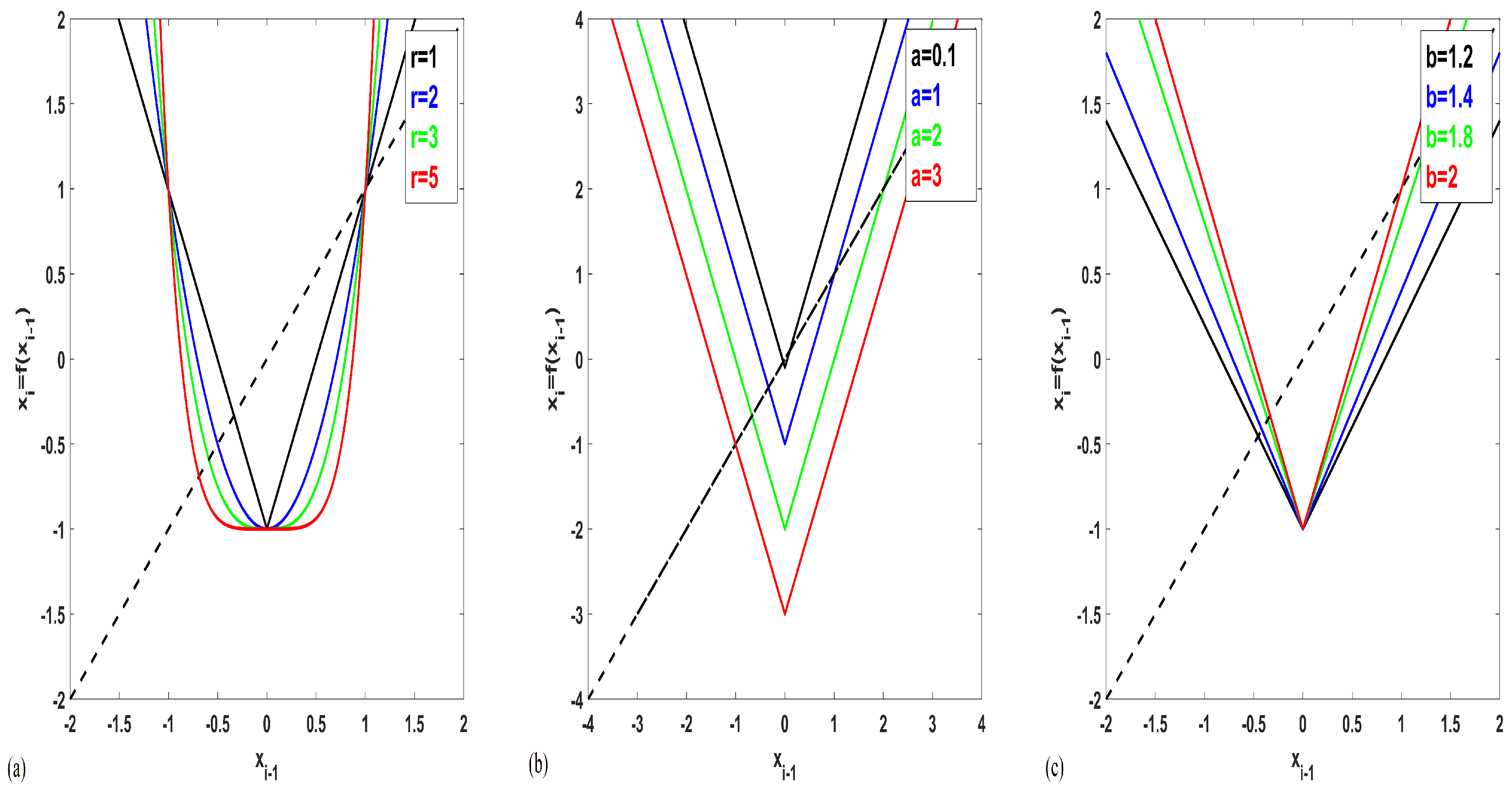
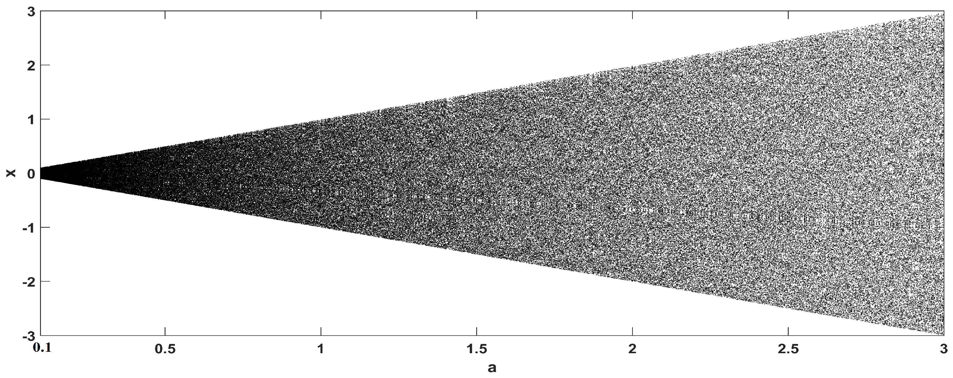
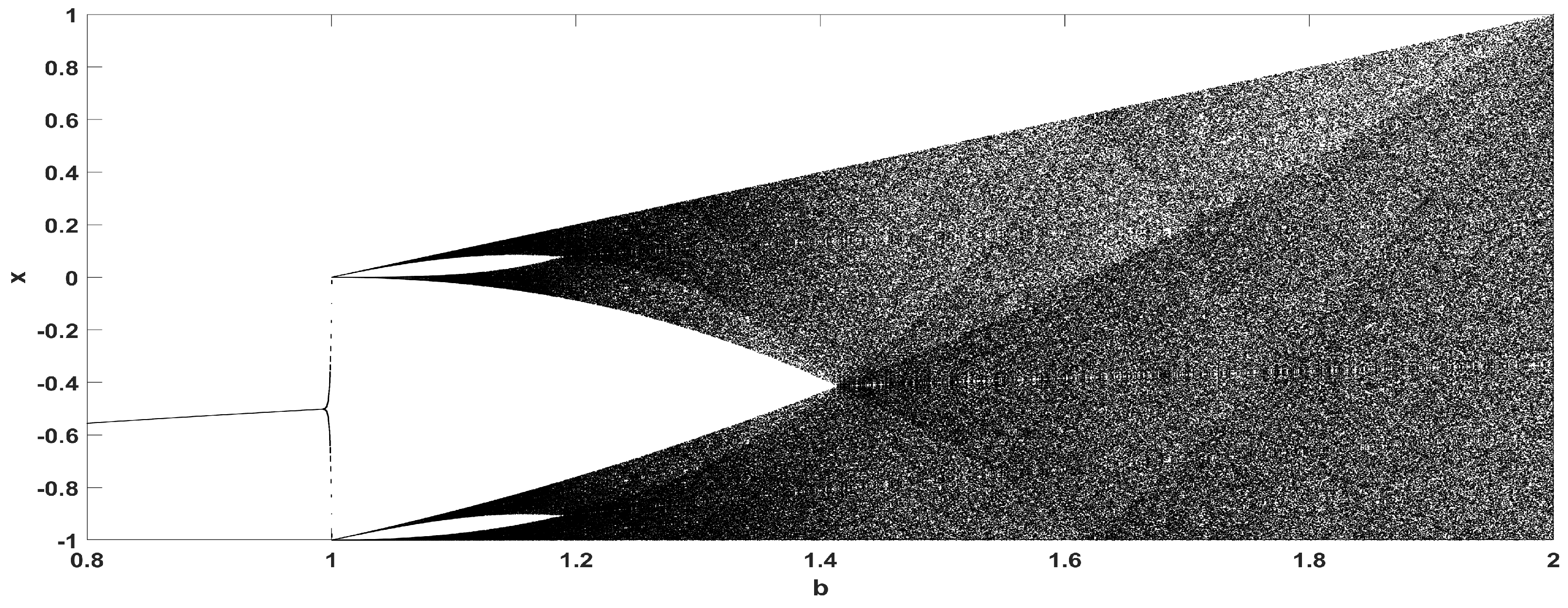
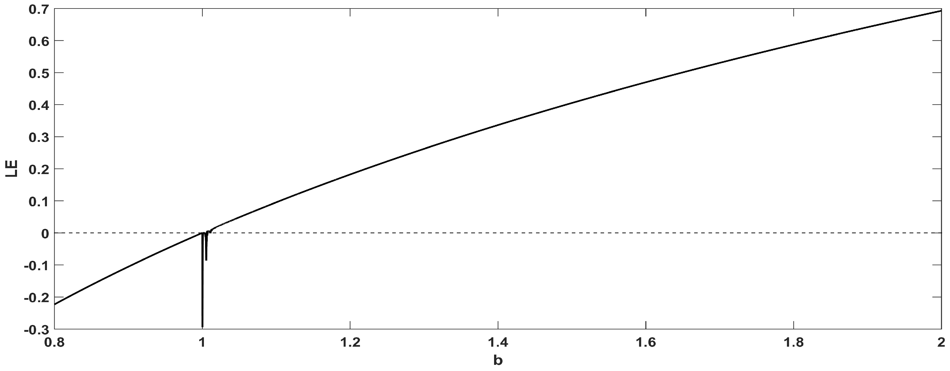
2. The Proposed Map
3. Application to Pseudo-Random Bit Generation
3.1. The Proposed Generator
- Step 1.
- First, the initial value of the proposed map is chosen, along with parameters b and a. These parameters constitute the secret keys of the algorithm. In addition, four bit sequences are initialized.
- Step 2.
- At each iteration, the decimal parts of , , , and are computed and compared to the threshold value of 0.5. Depending on the result, a ‘0’ or ‘1’ is produced and saved in , , , and respectively.
- Step 3.
- The bit sequences produced are combined into a single bitstream as .
3.2. Statistical Testing
3.2.1. NIST Tests
3.2.2. ENT Tests
- Entropy: The entropy of a random sequence should be close to 8.
- Optimum compression: This value should be close to zero.
- Chi square distribution rate: It should be between 10% and 90%.
- Arithmetic mean: It should be close to 127.5.
- Monte Carlo value for : It should approximate with a small error.
- Serial correlation coefficient: It should be close to zero for an uncorrelated sequence.
3.2.3. Correlation
3.2.4. Key Space
4. Application to Path Planning
4.1. The Proposed Chaotic Motion Generator
- Step 1.
- First, the initial value of the proposed map is chosen, along with parameters b and a. These three parameters constitute the secret keys of the algorithm. Then, four-bit sequences , , , and are initialized.
- Step 2.
- At each iteration, four bits are generated, , , , and , based on the procedure described in the previous section. Then, the bits are combined to generate a motion command for the robot in the horizontal plane, using the rules found in Table 5.
- Step 3.
- Based on the value of , the robot moves vertically up for or down for .
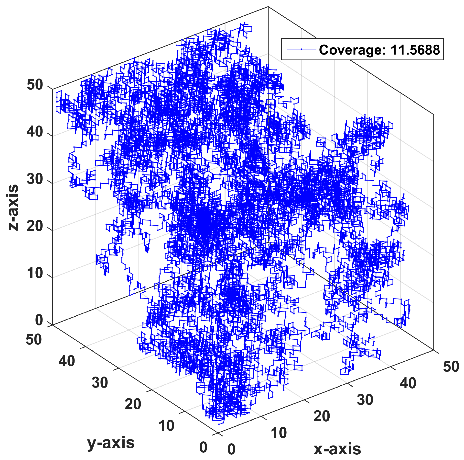
4.2. Coverage Performance
4.3. Adjusting the Discrete Steps to Smooth Motion
5. Conclusions
Author Contributions
Funding
Acknowledgments
Conflicts of Interest
References
- Strogatz, S.H. Nonlinear Dynamics and Chaos: With Applications to Physics, Biology, Chemistry, and Engineering; CRC Press: Boca Raton, FL, USA, 2018. [Google Scholar]
- Elaydi, S.N. Discrete Chaos: With Applications in Science and Engineering; CRC Press: Boca Raton, FL, USA, 2007. [Google Scholar]
- May, R.M. Simple mathematical models with very complicated dynamics. Nature 1976, 261, 459–467. [Google Scholar] [CrossRef]
- De la Fraga, L.G.; Torres-Pérez, E.; Tlelo-Cuautle, E.; Mancillas-López, C. Hardware implementation of pseudo-random number generators based on chaotic maps. Nonlinear Dyn. 2017, 90, 1661–1670. [Google Scholar] [CrossRef]
- Hua, Z.; Zhou, B.; Zhou, Y. Sine chaotification model for enhancing chaos and its hardware implementation. IEEE Trans. Ind. Electron. 2018, 66, 1273–1284. [Google Scholar] [CrossRef]
- Huang, X.; Liu, L.; Li, X.; Yu, M.; Wu, Z. A New Pseudorandom Bit Generator Based on Mixing Three-Dimensional Chen Chaotic System with a Chaotic Tactics. Complexity 2019, 2019. [Google Scholar] [CrossRef] [Green Version]
- Irfan, M.; Ali, A.; Khan, M.A.; Ehatisham-ul Haq, M.; Mehmood Shah, S.N.; Saboor, A.; Ahmad, W. Pseudorandom Number Generator (PRNG) Design Using Hyper-Chaotic Modified Robust Logistic Map (HC-MRLM). Electronics 2020, 9, 104. [Google Scholar] [CrossRef] [Green Version]
- François, M.; Grosges, T.; Barchiesi, D.; Erra, R. Pseudo-random number generator based on mixing of three chaotic maps. Commun. Nonlinear Sci. Numer. Simul. 2014, 19, 887–895. [Google Scholar] [CrossRef]
- Alawida, M.; Samsudin, A.; Teh, J.S. Enhanced digital chaotic maps based on bit reversal with applications in random bit generators. Inf. Sci. 2020, 512, 1155–1169. [Google Scholar] [CrossRef]
- Wang, L.; Cheng, H. Pseudo-Random Number Generator Based on Logistic Chaotic System. Entropy 2019, 21, 960. [Google Scholar] [CrossRef] [Green Version]
- Wang, Y.; Liu, Z.; Ma, J.; He, H. A pseudorandom number generator based on piecewise logistic map. Nonlinear Dyn. 2016, 83, 2373–2391. [Google Scholar] [CrossRef]
- Tutueva, A.V.; Nepomuceno, E.G.; Karimov, A.I.; Andreev, V.S.; Butusov, D.N. Adaptive chaotic maps and their application to pseudo-random numbers generation. Chaos Solitons Fractals 2020, 133, 109615. [Google Scholar] [CrossRef]
- Murillo-Escobar, M.; Cruz-Hernández, C.; Cardoza-Avenda no, L.; Méndez-Ramírez, R. A novel pseudorandom number generator based on pseudorandomly enhanced logistic map. Nonlinear Dyn. 2017, 87, 407–425. [Google Scholar] [CrossRef]
- Nakamura, Y.; Sekiguchi, A. The chaotic mobile robot. IEEE Trans. Robot. Autom. 2001, 17, 898–904. [Google Scholar] [CrossRef]
- Martins-Filho, L.S.; Macau, E.E. Patrol mobile robots and chaotic trajectories. Math. Probl. Eng. 2007. [Google Scholar] [CrossRef]
- Curiac, D.I.; Volosencu, C. A 2D chaotic path planning for mobile robots accomplishing boundary surveillance missions in adversarial conditions. Commun. Nonlinear Sci. Numer. Simul. 2014, 19, 3617–3627. [Google Scholar] [CrossRef]
- Li, C.; Song, Y.; Wang, F.; Liang, Z.; Zhu, B. Chaotic path planner of autonomous mobile robots based on the standard map for surveillance missions. Math. Probl. Eng. 2015, 2015. [Google Scholar] [CrossRef] [Green Version]
- Moysis, L.; Petavratzis, E.; Volos, C.; Nistazakis, H.; Stouboulos, I. A chaotic path planning generator based on logistic map and modulo tactics. Robot. Auton. Syst. 2020, 124, 103377. [Google Scholar] [CrossRef]
- Volos, C.K.; Kyprianidis, I.M.; Stouboulos, I.N. A chaotic path planning generator for autonomous mobile robots. Robot. Auton. Syst. 2012, 60, 651–656. [Google Scholar] [CrossRef]
- Nasr, S.; Mekki, H.; Bouallegue, K. A multi-scroll chaotic system for a higher coverage path planning of a mobile robot using flatness controller. Chaos Solitons Fractals 2019, 118, 366–375. [Google Scholar] [CrossRef]
- Volos, C.K.; Kyprianidis, I.; Stouboulos, I.; Stavrinides, S.; Anagnostopoulos, A. Anagnostopoulos, A. An Autonomous Mobile Robot Guided by a Chaotic True Random Bits Generator. In Chaos and Complex Systems; Springer: Berlin/Heidelberg, Germany, 2013; pp. 337–343. [Google Scholar]
- Volos, C.; Kyprianidis, I.; Stouboulos, I. Experimental investigation on coverage performance of a chaotic autonomous mobile robot. Robot. Auton. Syst. 2013, 61, 1314–1322. [Google Scholar] [CrossRef]
- Petavratzis, E.K.; Volos, C.K.; Moysis, L.; Stouboulos, I.N.; Nistazakis, H.E.; Tombras, G.S.; Valavanis, K.P. An Inverse Pheromone Approach in a Chaotic Mobile Robot’s Path Planning Based on a Modified Logistic Map. Technologies 2019, 7, 84. [Google Scholar] [CrossRef] [Green Version]
- Volos, C.K.; Prousalis, D.; Vaidyanathan, S.; Pham, V.T.; Munoz-Pacheco, J.; Tlelo-Cuautle, E. Kinematic control of a robot by using a non-autonomous chaotic system. In Advances and Applications in Nonlinear Control Systems; Springer: Berlin/Heidelberg, Germany, 2016; pp. 1–17. [Google Scholar]
- Gohari, P.S.; Mohammadi, H.; Taghvaei, S. Using chaotic maps for 3D boundary surveillance by quadrotor robot. Appl. Soft Comput. 2019, 76, 68–77. [Google Scholar] [CrossRef]
- Rosalie, M.; Danoy, G.; Chaumette, S.; Bouvry, P. Chaos-enhanced mobility models for multilevel swarms of UAVs. Swarm Evol. Comput. 2018, 41, 36–48. [Google Scholar] [CrossRef] [Green Version]
- Tawfik, M.A.; Abdulwahab, E.N.; Swadi, S.M. Specific Chaotic System and its Implementation in Robotic Field. Eng. Technol. J. 2015, 33, 2231–2243. [Google Scholar]
- Samuel, V.M.; Shehata, O.M.; Morgan, E.S.I. Chaos Generation for Multi-Robot 3D-Volume Coverage Maximization. In Proceedings of the 4th International Conference on Control, Mechatronics and Automation, Barcelona, Spain, 7–11 December 2016; ACM: New York, NY, USA, 2016; pp. 36–40. [Google Scholar]
- Tharwat, A.; Elhoseny, M.; Hassanien, A.E.; Gabel, T.; Kumar, A. Intelligent Bézier curve-based path planning model using Chaotic Particle Swarm Optimization algorithm. Clust. Comput. 2019, 22, 4745–4766. [Google Scholar] [CrossRef]
- Curiac, D.I.; Volosencu, C. Path planning algorithm based on Arnold cat map for surveillance UAVs. Def. Sci. J. 2015, 65, 483–488. [Google Scholar] [CrossRef] [Green Version]
- Zhou, Z.; Duan, H.; Li, P.; Di, B. Chaotic differential evolution approach for 3D trajectory planning of unmanned aerial vehicle. In Proceedings of the 2013 10th IEEE International Conference on Control and Automation (ICCA), Hangzhou, China, 12–14 June 2013; pp. 368–372. [Google Scholar]
- Mohanta, J.; Parhi, D.R.; Mohanty, S.; Keshari, A. A control scheme for navigation and obstacle avoidance of autonomous flying agent. Arab. J. Sci. Eng. 2018, 43, 1395–1407. [Google Scholar] [CrossRef]
- Moysis, L.; Petavratzis, E.; Volos, C.; Nistazakis, H.; Stouboulos, I.; Valavanis, K. A Chaotic Path Planning Method for 3D Area Coverage Using Modified Logistic Map and a Modulo Tactic. In Proceedings of the 2020 International Conference on Unmanned Aircraft Systems (ICUAS), Athens, Greece, 1–4 September 2020; pp. 220–227. [Google Scholar]
- He, H.; Cui, Y.; Lu, C.; Sun, G. Time Delay Chen System Analysis and Its Application. In Proceedings of the International Conference on Mechanical Design, Huzhou, China, 12–14 August 2019; Springer: Singapore, 2019; pp. 202–213. [Google Scholar]
- Sambas, A.; Vaidyanathan, S.; Mamat, M.; Sanjaya, W.M.; Rahayu, D.S. A 3-D novel jerk chaotic system and its application in secure communication system and mobile robot navigation. In Advances and Applications in Chaotic Systems; Springer: Cham, Switzerland, 2016; pp. 283–310. [Google Scholar]
- Vaidyanathan, S.; Sambas, A.; Mamat, M.; Sanjaya, W.M. A new three-dimensional chaotic system with a hidden attractor, circuit design and application in wireless mobile robot. Arch. Control Sci. 2017, 27, 541–554. [Google Scholar] [CrossRef] [Green Version]
- San-Um, W.; Ketthong, P. The generalization of mathematically simple and robust chaotic maps with absolute value nonlinearity. In Proceedings of the TENCON 2014-2014 IEEE Region 10 Conference, Bangkok, Thailand, 22–25 October 2014; pp. 1–4. [Google Scholar]
- Fong-In, S.; Kiattisin, S.; Leelasantitham, A.; San-Um, W. A partial encryption scheme using absolute-value chaotic map for secure electronic health records. In Proceedings of the 4th Joint International Conference on Information and Communication Technology, Electronic and Electrical Engineering (JICTEE), Chiang Rai, Thailand, 5–8 March 2014; pp. 1–5. [Google Scholar]
- Bovy, J. Lyapunov Exponents and Strange Attractors in Discrete and Continuous Dynamical Systems; Theoretical Physics Project; Technical Report; Katholieke Universiteit Leuven: Leuven, Belgium, 2004; Volume 9, pp. 1–19. [Google Scholar]
- Gayathri, J.; Subashini, S. A survey on security and efficiency issues in chaotic image encryption. Int. J. Inf. Comput. Secur. 2016, 8, 347–381. [Google Scholar]
- Kanso, A.; Ghebleh, M. A novel image encryption algorithm based on a 3D chaotic map. Commun. Nonlinear Sci. Numer. Simul. 2012, 17, 2943–2959. [Google Scholar] [CrossRef]
- Zhou, Y.; Bao, L.; Chen, C.P. A new 1D chaotic system for image encryption. Signal Process. 2014, 97, 172–182. [Google Scholar] [CrossRef]
- Tong, X.J. Design of an image encryption scheme based on a multiple chaotic map. Commun. Nonlinear Sci. Numer. Simul. 2013, 18, 1725–1733. [Google Scholar] [CrossRef]
- Tong, X.; Cui, M. Image encryption scheme based on 3D baker with dynamical compound chaotic sequence cipher generator. Signal Process. 2009, 89, 480–491. [Google Scholar] [CrossRef]
- Fu, C.; Chen, J.J.; Zou, H.; Meng, W.H.; Zhan, Y.F.; Yu, Y.W. A chaos-based digital image encryption scheme with an improved diffusion strategy. Opt. Express 2012, 20, 2363–2378. [Google Scholar] [CrossRef] [PubMed]
- Chen, J.X.; Zhu, Z.L.; Yu, H. A fast chaos-based symmetric image cryptosystem with an improved diffusion scheme. Optik 2014, 125, 2472–2478. [Google Scholar] [CrossRef]
- Wong, K.W.; Kwok, B.S.H.; Yuen, C.H. An efficient diffusion approach for chaos-based image encryption. Chaos Solitons Fractals 2009, 41, 2652–2663. [Google Scholar] [CrossRef] [Green Version]
- Fu, C.; Meng, W.H.; Zhan, Y.F.; Zhu, Z.L.; Lau, F.C.; Chi, K.T.; Ma, H.F. An efficient and secure medical image protection scheme based on chaotic maps. Comput. Biol. Med. 2013, 43, 1000–1010. [Google Scholar] [CrossRef]
- Rukhin, A.; Soto, J.; Nechvatal, J.; Smid, M.; Barker, E. A Statistical Test Suite for Random and Pseudorandom Number Generators for Cryptographic Applications; Technical Report; Booz-Allen and Hamilton Inc. Mclean Va: Gaithersburg, MD, USA, 2001. [Google Scholar]
- Walter, J. ENT: A Pseudo Random Number Sequence Test Program. 2008. Available online: https://www.fourmilab.ch/random/ (accessed on 22 July 2021).
- Zhang, Z.; Wang, Y.; Zhang, L.Y.; Zhu, H. A novel chaotic map constructed by geometric operations and its application. Nonlinear Dyn. 2020, 102, 2843–2858. [Google Scholar] [CrossRef]
- Alvarez, G.; Li, S. Some basic cryptographic requirements for chaos-based cryptosystems. Int. J. Bifurc. Chaos 2006, 16, 2129–2151. [Google Scholar] [CrossRef] [Green Version]
- Zeraoulia, E. Robust Chaos and Its Applications; World Scientific: Singapore, 2012; Volume 79. [Google Scholar]
- Hua, Z.; Zhou, Y. Exponential chaotic model for generating robust chaos. IEEE Trans. Syst. Man, Cybern. Syst. 2019, 51, 3713–3724. [Google Scholar] [CrossRef]
- Foo, J.L.; Knutzon, J.; Kalivarapu, V.; Oliver, J.; Winer, E. Path planning of unmanned aerial vehicles using B-splines and particle swarm optimization. J. Aerosp. Comput. Inform. Commun. 2009, 6, 271–290. [Google Scholar] [CrossRef]
- Koyuncu, E.; Inalhan, G. A probabilistic B-spline motion planning algorithm for unmanned helicopters flying in dense 3D environments. In Proceedings of the 2008 IEEE/RSJ International Conference on Intelligent Robots and Systems, Nice, France, 22–26 September 2008; pp. 815–821. [Google Scholar]
- Jung, D.; Tsiotras, P. On-line path generation for unmanned aerial vehicles using B-spline path templates. J. Guid. Control. Dyn. 2013, 36, 1642–1653. [Google Scholar] [CrossRef] [Green Version]
- Moysis, L. Introduction to Computer Aided Geometric Design—A Student’s Companion with Matlab Examples; MathWorks, Inc.: Natick, MA, USA, 2018. [Google Scholar]
- Piegl, L.; Tiller, W. The NURBS Book; Springer: Berlin/Heidelberg, Germany, 2012. [Google Scholar]


| Reference | Map | Number of Parameters |
|---|---|---|
| Elaydi [2] | 1 () | |
| San-Um and Ketthong [37] | 1 | |
| San-Um and Ketthong [37] | 1 | |
| San-Um and Ketthong [37] | 1 | |
| San-Um and Ketthong [37] | 1 | |
| Fong-In et al. [38] | 2 |
| Algorithm | Performance (B/ms) |
|---|---|
| Proposed approach | 2642 |
| Kanso et al. [41] | 2023 |
| Zhou et al. [42] | 407.1 |
| Tong et al. [43] | 181.09548 |
| Xiaojun et al. [44] | 121.7448027 |
| Fu et al. [45] | 78 |
| Chen et al. [46] | 41 |
| Wong et al. [47] | 40.37 |
| Fu et al. [48] | 11 |
| If , the Test is Successful Passed | |||
|---|---|---|---|
| No. | Statistical Test | p-Value | Proportion |
| 1 | Frequency | 0.392456 | 40/40 |
| 2 | Block Frequency | 0.875539 | 40/40 |
| 3 | Cumulative Sums | 0.186566 | 40/40 |
| 4 | Runs | 0.484646 | 40/40 |
| 5 | Longest Run | 0.689019 | 40/40 |
| 6 | Rank | 0.534146 | 40/40 |
| 7 | FFT | 0.213309 | 40/40 |
| 8 | Non-Overlapping Template | 0.311542 | 39/40 |
| 9 | Overlapping Template | 0.275709 | 39/40 |
| 10 | Universal | 0.213309 | 39/40 |
| 11 | Approximate Entropy | 0.964295 | 40/40 |
| 12 | Random Excursions | 0.637119 | 23/24 |
| 13 | Random Excursions Variant | 0.162606 | 24/24 |
| 14 | Serial | 0.637119 | 40/40 |
| 15 | Linear Complexity | 0.437274 | 40/40 |
| No. | Statistical Test | Result |
|---|---|---|
| 1 | Entropy | 7.999987 |
| 2 | Optimum Compression | 0% |
| 3 | Chi-Square | 15.37% |
| 4 | Arithmetic mean | 127.4871 |
| 5 | Monte Carlo value for | 3.1420352 (0.01% error) |
| 6 | Serial Correlation Coefficient | 0.000244 |
| Motion in 8 Directions | |
|---|---|
| Bits | Motion command |
| 000 | up |
| 100 | up-right |
| 110 | right |
| 101 | down-right |
| 011 | down |
| 111 | down-left |
| 001 | left |
| 010 | up-left |
Publisher’s Note: MDPI stays neutral with regard to jurisdictional claims in published maps and institutional affiliations. |
© 2021 by the authors. Licensee MDPI, Basel, Switzerland. This article is an open access article distributed under the terms and conditions of the Creative Commons Attribution (CC BY) license (https://creativecommons.org/licenses/by/4.0/).
Share and Cite
Moysis, L.; Rajagopal, K.; Tutueva, A.V.; Volos, C.; Teka, B.; Butusov, D.N. Chaotic Path Planning for 3D Area Coverage Using a Pseudo-Random Bit Generator from a 1D Chaotic Map. Mathematics 2021, 9, 1821. https://doi.org/10.3390/math9151821
Moysis L, Rajagopal K, Tutueva AV, Volos C, Teka B, Butusov DN. Chaotic Path Planning for 3D Area Coverage Using a Pseudo-Random Bit Generator from a 1D Chaotic Map. Mathematics. 2021; 9(15):1821. https://doi.org/10.3390/math9151821
Chicago/Turabian StyleMoysis, Lazaros, Karthikeyan Rajagopal, Aleksandra V. Tutueva, Christos Volos, Beteley Teka, and Denis N. Butusov. 2021. "Chaotic Path Planning for 3D Area Coverage Using a Pseudo-Random Bit Generator from a 1D Chaotic Map" Mathematics 9, no. 15: 1821. https://doi.org/10.3390/math9151821