Article

Geological Modeling Method Based on the Normal Dynamic Estimation of Sparse Point Clouds

School of Resources and Safety Engineering, Central South University, Changsha 410083, China
*
Author to whom correspondence should be addressed.
Mathematics 2021, 9(15), 1819; https://doi.org/10.3390/math9151819
Submission received: 4 July 2021 / Revised: 25 July 2021 / Accepted: 29 July 2021 / Published: 31 July 2021

Abstract

:
The effect of geological modeling largely depends on the normal estimation results of geological sampling points. However, due to the sparse and uneven characteristics of geological sampling points, the results of normal estimation have great uncertainty. This paper proposes a geological modeling method based on the dynamic normal estimation of sparse point clouds. The improved method consists of three stages: (1) using an improved local plane fitting method to estimate the normals of the point clouds; (2) using an improved minimum spanning tree method to redirect the normals of the point clouds; (3) using an implicit function to construct a geological model. The innovation of this method is an iterative estimation of the point cloud normal. The geological engineer adjusts the normal direction of some point clouds according to the geological law, and then the method uses these correct point cloud normals as a reference to estimate the normals of all point clouds. By continuously repeating the iterative process, the normal estimation result will be more accurate. Experimental results show that compared with the original method, the improved method is more suitable for the normal estimation of sparse point clouds by adjusting normals, according to prior knowledge, dynamically.

1. Introduction

Geological modeling mainly studies how to infer the geometric model of the original geological body described by sparse geological sampling data. Geological sampling data has three major characteristics, which are multi-source, sparse, and uneven. It is a huge challenge to use limited sampling data to infer and predict the distribution trend of a model at unknown regions, and the corresponding modeling results also have greater uncertainty. The establishment of a reliable three-dimensional geological model (especially the ore body model) is an important basis for calculation of mineral resources, reserves, and mining design.
In recent years, an implicit modeling [1,2,3,4,5] method that uses implicit functions to implicitly express geometric model of geological bodies has attracted increased attention. Implicit here has two meanings: that the method uses an implicit function to represent the three-dimensional model; and that the three-dimensional model represented by the implicit function cannot be directly displayed in the three-dimensional view, as it needs to be converted into a mesh model by using the surface reconstruction method. At present, implicit modeling has made great breakthroughs in method and theory. Researchers [6,7,8,9,10] have proposed a variety of implicit modeling methods based on different interpolation methods and constraint rules. However, this method is still difficult to interpolate sparse geological data. Lacking of a reliable theory of geological rules suitable for ore body modeling, the implicit modeling method has not been widely promoted and applied in complex ore body modeling.
Implicit modeling methods generally control the shape of the model by constructing interpolation constraints, and the quality of the modeling results depends largely on the determination of the normal direction of the constraint points [11]. Many recent surface reconstruction algorithms [12,13,14,15] also require normal information to obtain faithful reconstructions. Currently, the point clouds normal estimation methods can be divided into three types, namely methods based on local surface fitting, Delaunay/Voronoi, robust statistics.
Hoppe et al. [16] proposed a classic method based on local surface fitting. This method assumes that the surface of the sampled data points is smooth, and that the local surface of any sampled data point can be well-fitted with a plane. A local fitting plane in the sense of least squares is calculated using the neighborhood points around the point to be solved, and the normal direction of the fitting plane is the normal direction of the point to be solved. Literature [17] improves the method proposed by Hoppe et al. Each neighborhood point is given a Gaussian weight, which means that neighborhood points that are closer to the point to be solved will have a greater impact. Literature [18] proposed another weight representation method, which takes the distance from the neighborhood point to the projection point of the point to be solved on the fitting plane as the weight. However, the method based on local plane fitting needs to specify the size of the neighborhood, and different neighborhood sizes will produce different normal estimation results [19]. Aiming at the problem of how to determine the optimal neighborhood, literature [20] comprehensively analyzes the noise, sampling density, curvature, and other factors of the point clouds data, and obtains the upper bound of the error between the estimated normal directions and the true normal directions. An analytical model is constructed, which can iteratively find the optimal neighborhood size for each point, given the noise level of the model.
The method based on Delaunay/Voronoi was first proposed by Amenta et al. [21]. This method involves constructing a Voronoi diagram of the point clouds and performing Delaunay triangulation. For a point located in a convex hull, the normal direction is the line connecting the point and the Voronoi vertex (called pole) farthest from the point in the Voronoi lattice where the point is located. If the point is exactly on the convex hull, then the point at the infinity outside the convex hull in the direction of the average normal of the convex hull adjacent to the point is taken as the pole. The method proposed by Amenta et al. is only suitable for noise-free point clouds data. Literature [22] improved the method proposed by Amenta et al.; thus, it can process point clouds data with noise. Literature [23] combines the method based on local plane fitting and the method based on the Voronoi diagram. First, calculate the fitting plane formed by all the points in the Voronoi lattice where each point is located, and then the normal direction of this plane is taken as the normal direction of the point to be solved.
The robust statistics-based methods use techniques in robust statistics to deal with noise, outliers, and sharp parts in point clouds data [24]. Literature [25] proposed a robust moving least squares method for reconstructing the surface based on the forward search mechanism. The method divides the neighborhood of each point into multiple sub-areas without outliers, and then uses the moving least squares method to reconstruct the surface in each sub-area. At the same time, the normal direction of each point can be reconstructed from the smooth surface of the piece. Literature [26] proposed a robust normal estimation method that can handle the sharp part of the point clouds. The method is similar to the moving least squares method. The main difference is that the method only requires a single plane in the neighborhood where each point is located, instead of dividing the neighborhood into several smooth regions.
In this paper, the problem of geological modeling based on geological sampling data is transformed into the problem of determining the normal directions of sparse and uneven point clouds. Because the geological contact points extracted based on geological sampling data are sparse and uneven, the normals obtained by the traditional normal estimation methods are generally difficult to meet the requirements of geological modeling. Compared with dense point clouds data, the normal estimation results of sparse and uneven point clouds are more uncertain. Conversely, only relying on the spatial position relationship of the point clouds data to estimate the normals of the geological contact points ignores the geological conditions of the corresponding geological environment. It is necessary to provide a method for geological engineers to dynamically adjust the normal estimation result interactively. Therefore, the normals of the known points (allowing geological engineers to determine the normal of certain points according to the geological rules) and the spatial position relationship between the borehole samples should be considered for the normal estimation of the point clouds and the normal redirection.
This paper proposes an implicit geological modeling method based on the normal dynamic estimation of sparse point clouds. This method allows the geological engineer to interactively adjust the normals of certain points according to the geological rules, and the method can automatically update the normals of the neighboring points where the adjustment point is located. It also allows the geological engineer to interactively adjust the normal polarity directions of certain points according to the geological rules, and the method can automatically update the normal polarity directions of the neighboring points in which the adjustment point is located. In addition, the method proposed in this paper is also suitable for dense point cloud normal estimation and modeling tasks, such as the usual three-dimensional surface reconstruction tasks.
The remainder of this paper is organized as follows: Section 2 describes in detail the proposed method. Section 3 presents the experimental results. Section 4 discusses the method proposed in this paper. Finally, Section 5 concludes this paper.

2. Methods

The method proposed in this paper mainly consists of the following three steps. Figure 1 shows the overall flow of the method.
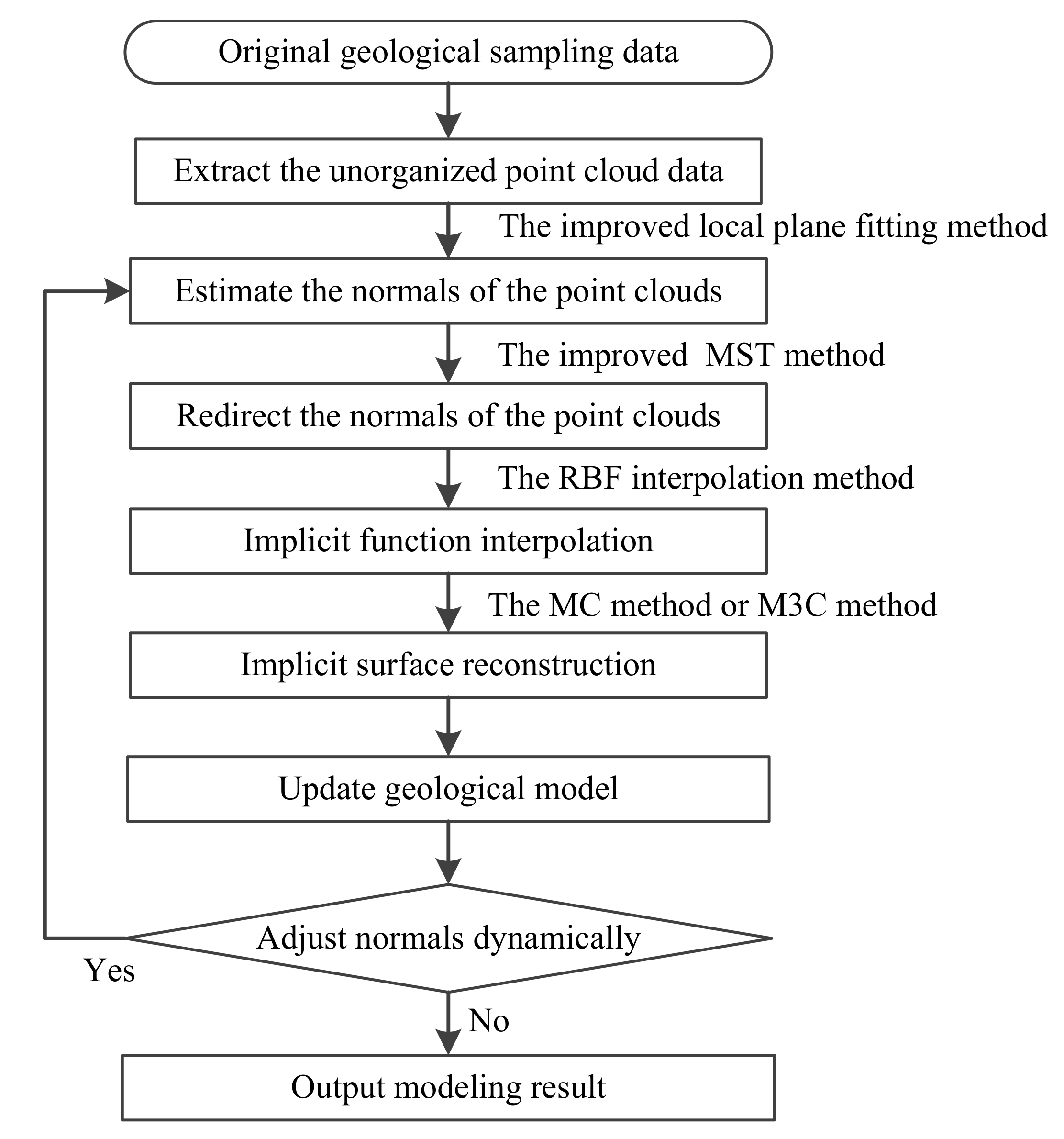
1. Extracting the unorganized point clouds data from the original geological sampling data and using the improved local plane fitting method to estimate the normal of the point clouds. To ensure that the normals of the point clouds all face the exterior of the geological model, the improved minimum spanning tree (MST) method is used to redirect the normals of the point clouds.
2. The interpolation constraints are constructed based on the oriented point clouds data, and the radial basis function (RBF) interpolation method [27] is used to obtain the implicit function that represents the geological model. To obtain the polygonal geological model, reconstruct the surface of the interpolated implicit function using the marching cubes (MC) method [28,29] or the multiple marching cubes (M3C) method [30].
3. The geological engineer is allowed to adjust the normals to obtain certain points with known normal directions, according to prior knowledge, dynamically. Then, the updated geological model can be reconstructed by re-executing the first and second steps above.
This paper focuses on the dynamic estimation of the normal of the point clouds. In the geological modeling task, the geological engineer is allowed to dynamically adjust the normals of certain data points according to the geological rules. The point, whose normal has been adjusted manually, will affect the normal estimation of other points. First, this paper improves the point clouds normal estimation method based on the local fitting plane. It can be assumed that the normals tend to be in the same direction if their points are relatively close. Therefore, if the normal vector of the point to be solved computes inner product with the vector in the tangent plane of the neighboring point with a known normal, the result should be close to zero, which is added to the objective function of constructing the local fitting plane as a constraint item. Second, this paper improves the MST-based normal redirection method proposed by Hoppe et al. [16]. The normal directions of the points that have been dynamically adjusted to normal are viewed as the right directions, which can be used as the starting point of the normal propagation in the improved MST method.

2.1. Normal Estimation

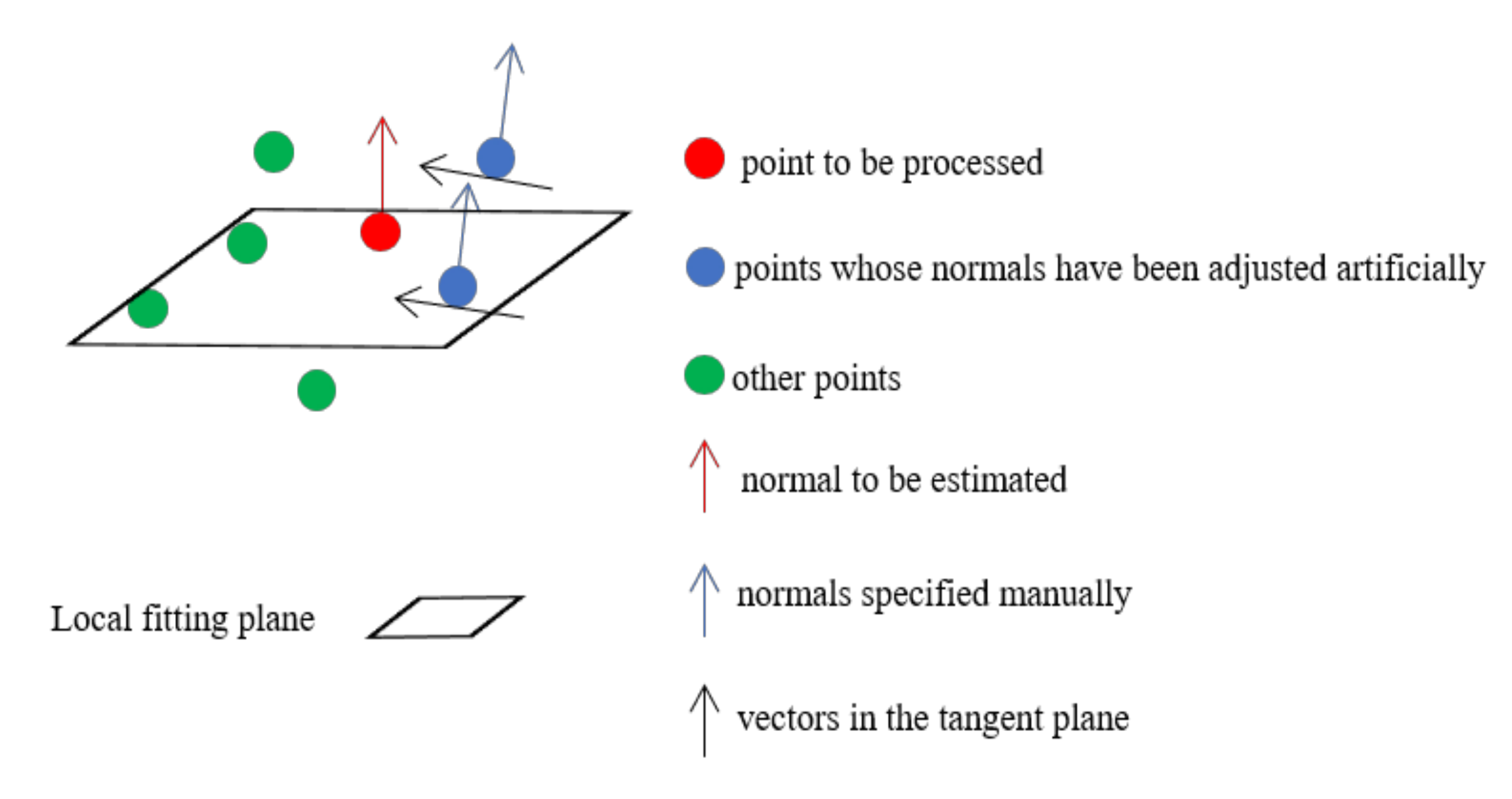
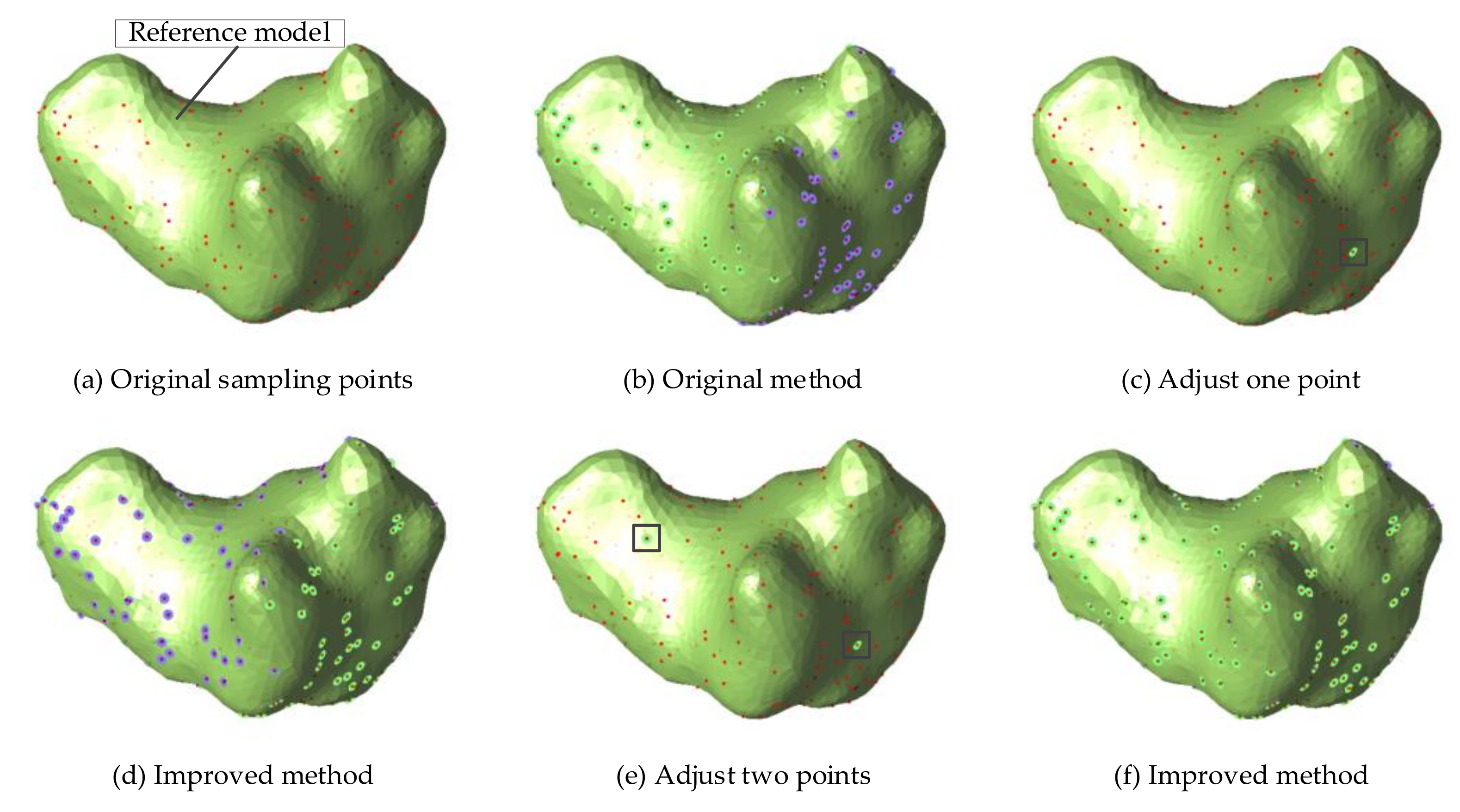
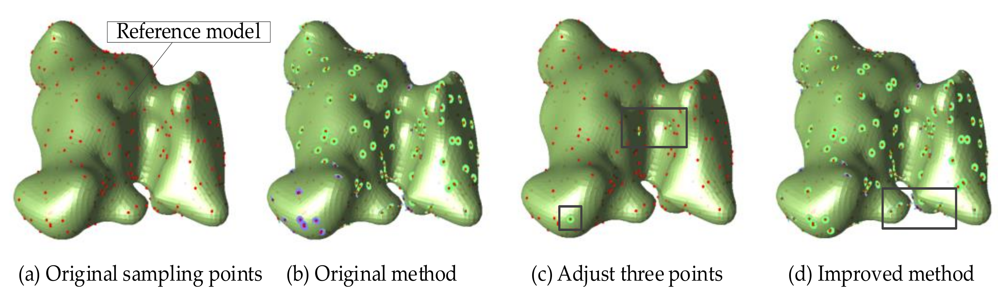
This paper improves the point clouds normal estimation method based on local plane fitting to cause the result of normal estimation to be more accurate. The traditional method based on local plane fitting does not consider the influence of the points whose normals have been adjusted manually on the normal estimation of the rest of the point clouds. For geological modeling, the normals of certain points can be adjusted manually, and the points whose normals have been adjusted manually will affect the normal estimation of the neighboring points, as shown in Figure 2. For neighboring points whose normals have been adjusted manually, a tangent plane is calculated according to the normal of the neighboring point, and the plane is marked as a reference plane. Since the local plane fitting method assumes that the local neighborhood of any point can be well-fitted with a plane, the normal of the point to be solved should be perpendicular to this reference plane. According to this assumption, the inner product of a normal vector of the point to be solved and a vector v j on the reference plane should be close zero. It is a constraint imposed on the point to be solved by those points whose normals have been adjusted manually.
If the distance between two points is close enough, the normals of the two points should tend to be in the same direction. Therefore, the normals of the two points should be perpendicular to the same plane. At the same time, because the distance from each neighborhood point to the point to be solved is different, each neighborhood point has a different influence on the point to be solved. This paper uses the inverse distance weight to express the different degrees of influence. The neighborhood points that are close to the point to be solved have a greater influence, while the neighborhood points that are far away from the point to be solved have less influence.
In the calculation process, the first step is to calculate the coordinates of a vector v j in the reference plane. The second step is to perform the inner product between the vector v j and normal vector of the point to be solved and assign the corresponding inverse distance weight. Then, the result is introduced as a constraint item into the objective function based on the local plane fitting method. By solving the improved objective function, the normal estimation result will be more accurate. The calculation formula for the coordinates of vector v j is as follows:
x × a + y × b + z × c = 0
where x , y , z represent the coordinates of vector v j to be calculated, and a , b , c represent the normal coordinates of the point whose normal direction has been adjusted manually.
The coordinates of vector v j have three components to be solved, and Formula (1) has only one equation. Therefore, it is necessary to manually specify two components. All the neighboring points of the point to be solved are numbered sequentially ( 1 ~ N ). Number value (n) of the neighboring point and number 1 are used to represent the two components of corresponding vector v j . The third component can be solved by Formula (1). After obtaining the coordinates of vector v j , it needs to be normalized.
In the process of solving the Formula (1), we need to consider that a certain component of the coordinates is equal to zero. Therefore, it is necessary to compare the absolute value of three components to find the component with the largest absolute value. If ∣ a b ∣ and ∣ a c ∣, then the maximum of three components is x component and its value must not be zero. Therefore, the coordinates can be set to the form of v j ( x , 1, n), and the value of x can be calculated according to Formula (2).
x = b c a
If ∣ b a ∣ and ∣ b c ∣, then maximum of three components is y component and its value must not be zero. Therefore, the coordinates can be set to the form of v j (1, y , n ), and the value of y can be calculated according to Formula (3).
y = a c b
If ∣ c b ∣ and ∣ c a ∣, then the maximum of the three components is z component and its value must not be zero. Therefore, the coordinates can be set to the form of v j (1, n ,   z ), and the value of z can be calculated according to Formula (4).
z = a b c
The goal of the original method based on local plane fitting is to minimize the sum of distance from each neighborhood point to the fitting plane. The improvement of this paper is that when the normal of the neighborhood point is adjusted manually, a vector v j needs to be selected in the tangent plane of the neighborhood point to compute inner product with the normal vector of the point to be solved. The result of the inner product should be given corresponding to the inverse distance weight and then added to the objective function as a constraint item. The vector formed by the neighborhood point and the point to be solved is not normalized; thus, its own length has an impact on the result of the inner product operation. However, the vector v j is a normalized vector; thus, it should be multiplied by a length coefficient d j , which represents the distance from a corresponding neighborhood point to the point to be solved. The improved objective function is shown in Formula (5):
min ( i = 1 n ( λ i · x i x 0 ) T · n 2 + j = 1 m λ j · d j · v j · n 2 ) s . t . n T · n = 1
λ i = 1 d i 2 i = 1 n 1 d i 2
λ j = 1 d j 2 j = 1 m 1 d j 2
Among them, x i represents the neighborhood point of the point to be solved; x 0 represents the point to be solved; n represents normal of the point to be solved, which is also normal of the fitting plane; n represents the total number of all neighborhood points; v j represents the vector in the tangent plane of a neighboring point whose normal direction has been adjusted manually; m represents total number of neighboring points whose normals have been adjusted manually; λ i and λ j represent the inverse distance weight; d i represents the distance from the i-th neighborhood point to the point to be solved; d j represents the distance from the j-th neighborhood point whose normal direction has been adjusted manually to the point to be solved.
Further derivation of the objective function:
y i = x i x 0
min ( i = 1 n n T λ i y i λ i y i T n + j = 1 m n T λ j d j v j λ j d j v j T n ) s . t . n T · n = 1
min ( n T ( i = 1 n y i y i T + j = 1 m v j v j T ) n ) s . t . n T · n = 1
where y i = λ i y i , v j = λ j d j v j .
min n T Y Y T + V V T n s . t . n T · n = 1
where Y = y 1   y 2     y n , V = v 1   v 2     v n .
C = Y Y T + V V T
The final form of the objective function is:
min n T C n s . t . n T · n = 1
The improved objective function is the same in form as the original objective function based on the local surface fitting method; thus, its solution method is the same. The three eigenvectors are obtained by eigenvalue decomposition of matrix C , and the eigenvector corresponding to the smallest eigenvalue is the normal vector to be solved.

2.2. Consistent Normal Orientation

The normal obtained by the local plane fitting method is ambiguous, because only the line where the normal is located is obtained. The normal direction is not determined. In geological modeling, the correct normal direction of the point clouds should be toward the outside of the model. When the normal direction of the point clouds is toward the inside of the model, the normal direction needs to be flipped. The minimum spanning tree method proposed by Hoppe et al. [16] is a common normal redirection method. This method uses the sampled data points and the adjacent relationship between the points to construct a Riemann graph. The cost of the edges of the Riemann graph is 1 n i · n j , where n i and n j are respectively the unit normal vector of point p i and point p j . If the normal directions of two adjacent points are the same, the cost of the edge is small. The normal propagation is performed by calculating the minimum spanning tree of the Riemann graph and traversing the minimum spanning tree.
Although researchers have improved this method [31,32], this method has inherent flaws. First, when the normal directions of two adjacent points are both toward the inside of the model, the inner product of the normal vectors of the two points is greater than 0, and the normal directions of the two points will not be flipped to facing the correct direction outside the model. Second, when selecting the starting point of normal propagation, if the normal direction of the starting point is toward the inside of the model, it will have a wrong effect on the normal directions of the following points. In this paper, the normal direction of certain points can be adjusted dynamically. The normal directions of the points whose normal directions are adjusted are correct and can be used as the starting point of the normal propagation process. This paper improves the minimum spanning tree method to produce the result of normal propagation to be more accurate. 
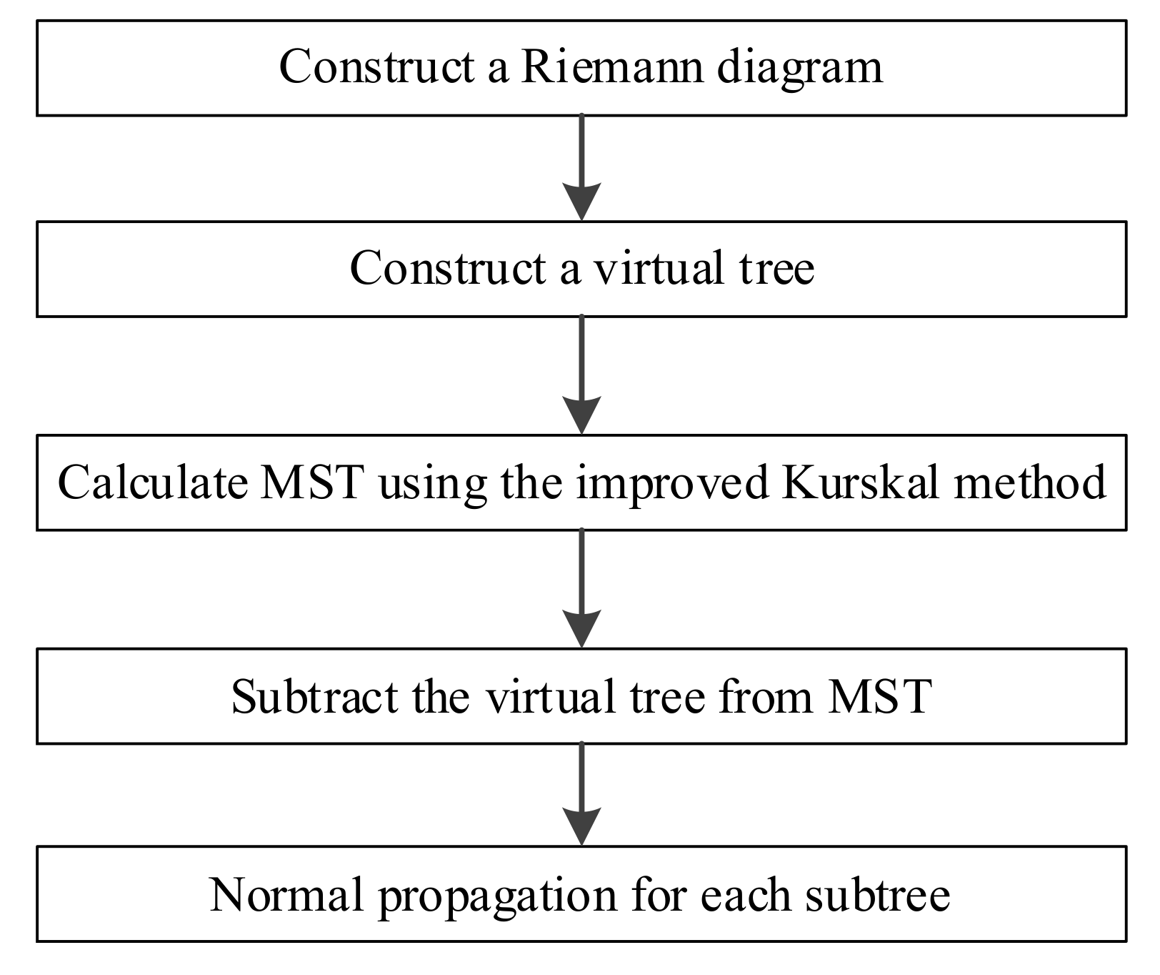
Figure 3 shows the process of the improved minimum spanning tree method.
The first step of the method is to construct a Riemann graph. All points in the point clouds are regarded as the vertexes of the Riemann graph. If two points p i and p j are each other’s k neighboring points, then the adjacency relationship between the two points is regarded as the edge of the Riemann graph. After constructing the Riemann graph, the cost of the edges is set to 1 n i · n j , where n i and n j are respectively the unit normal vector of point p i and point p j .
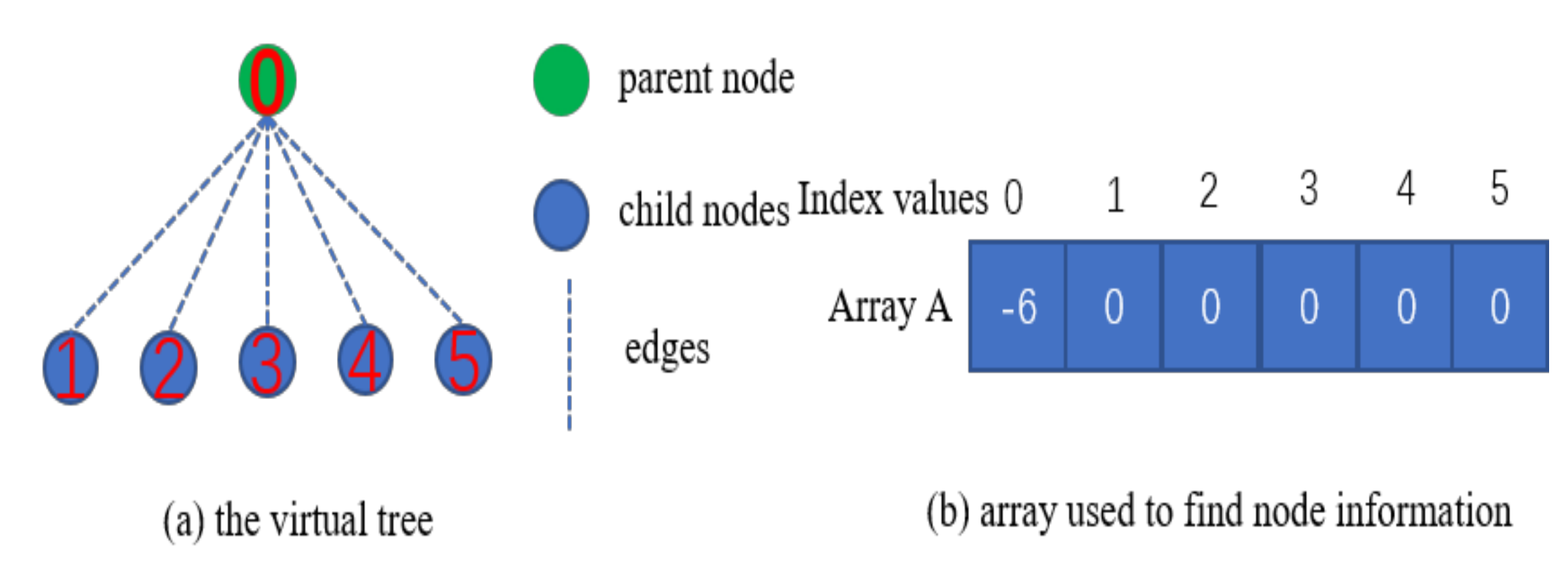
The second step of the method is to construct a virtual tree TV for those points whose normal has been adjusted manually. By using a set P to represent those points whose normal has been adjusted manually, a point p in the set P is selected as the parent node of all the remaining points in the set P, and the remaining points in the set P are all child nodes of the node p. By using these nodes to construct a virtual tree, each node in the tree is numbered in order ( 0 ~ N 1 ), where N represents the total number. Figure 4a shows the structure of the virtual tree. This paper uses an array A to store the node information using the method of union-find sets. The index value i of each element in the array corresponds to the node numbered i in the virtual tree, and the element value corresponding to each index value i in the array represents the number of the parent node of the node numbered i in the virtual tree. The parent node in the virtual tree does not have its own parent node. To ensure that the element with index 0 in the array exists, this paper assumes a virtual parent node for the parent node in the virtual tree, and the corresponding value is N . Figure 4b shows the structure of array A.
The third step of the method is to calculate the minimum spanning tree TM. This paper presents an improved Kruskal method. The initial state of the Kruskal method only contains all vertexes, and each vertex is regarded as an independent tree to form a forest. At each iteration, a minimum cost edge that satisfies the condition is selected to be added to the forest. Finally, the minimum spanning tree is obtained.
This paper modifies the initial state of the Kruskal method. The virtual tree and other isolated points in the Riemann graph form the initial state of the improved Kruskal method. Then, the Kruskal method is used to add edges to obtain the minimum spanning tree. 
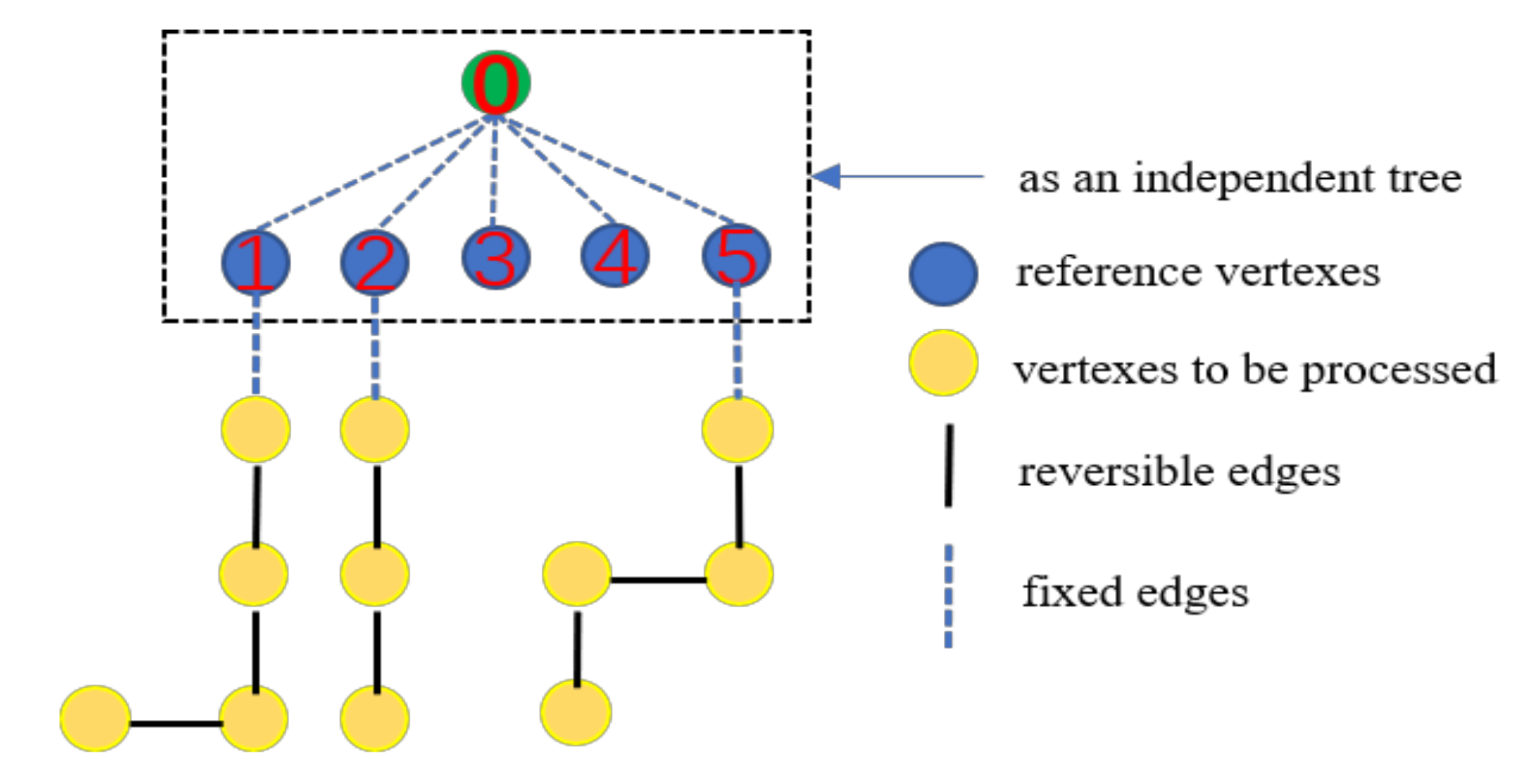
Figure 5 shows the structure of this minimum spanning tree.
There are two types of edges in the minimum spanning tree. One is that the normal of the two vertexes connected on the edge has not been adjusted manually. It can be represented as a reversible edge, which means that the normal of the two vertexes on the edge needs to be processed. The other is that the normal of one vertex of the two vertexes connected on the edge has been adjusted manually. It can be represented as a fixed edge, which means that the normal of a vertex on the edge is correct. The points on the fixed edges whose normals have been adjusted manually are selected as starting points in the process of normal propagation, which are represented as reference vertexes.
The fourth step of the method is to remove virtual tree TV from minimum spanning tree TM to obtain multiple subtrees Ti. The normals of nodes in the virtual tree TV have been adjusted manually. The normals of nodes in the virtual tree can be considered to be facing outside of the model correctly, and there is no need to flip them in the process of normal propagation. Therefore, before performing normal propagation, the virtual tree TV needs to be removed from the minimum spanning tree TM to obtain multiple subtrees Ti. The normal propagation is performed by selecting the reference vertexes on the fixed edges of the subtrees as the starting points. 
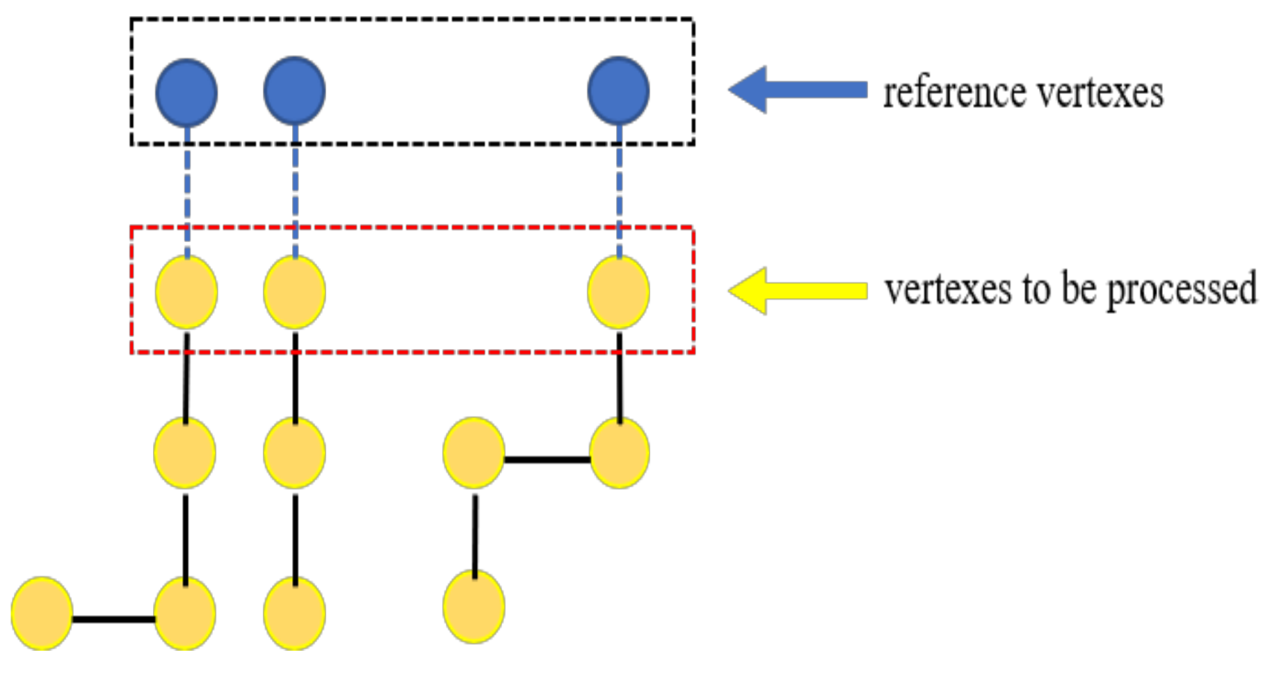
Figure 6 shows the structure of the subtrees.
The fifth step of the method is to perform normal propagation. Each subtree has a fixed edge, which connects a reference vertex and a to-be-processed vertex. For each subtree, a reference vertex is used as the starting point, and the breadth-first search method is used to traverse all nodes of the tree. If the inner product of the normal vectors of two adjacent vertexes is negative, the normal toward the inside of the model is flipped to make it toward the outside of the model.

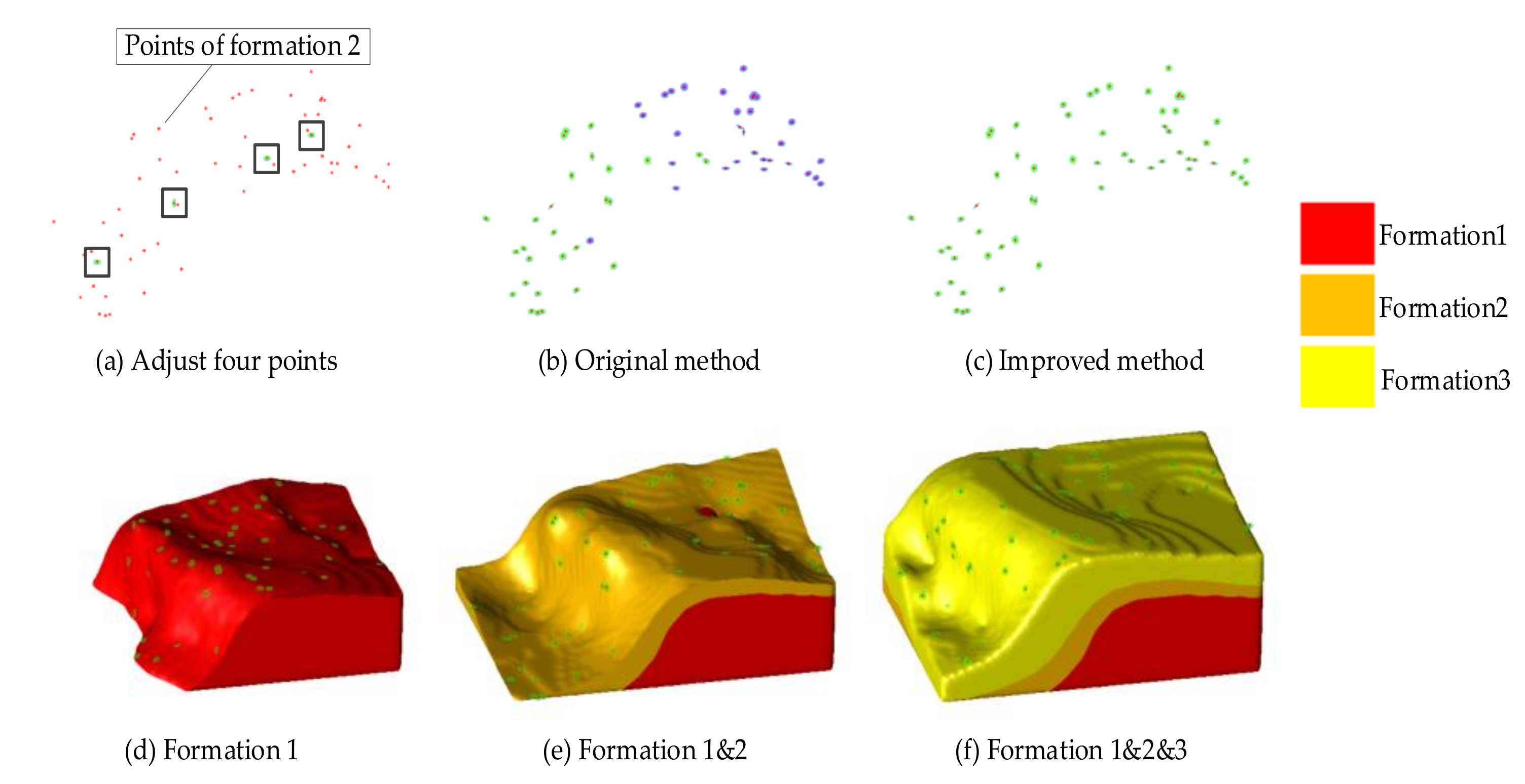
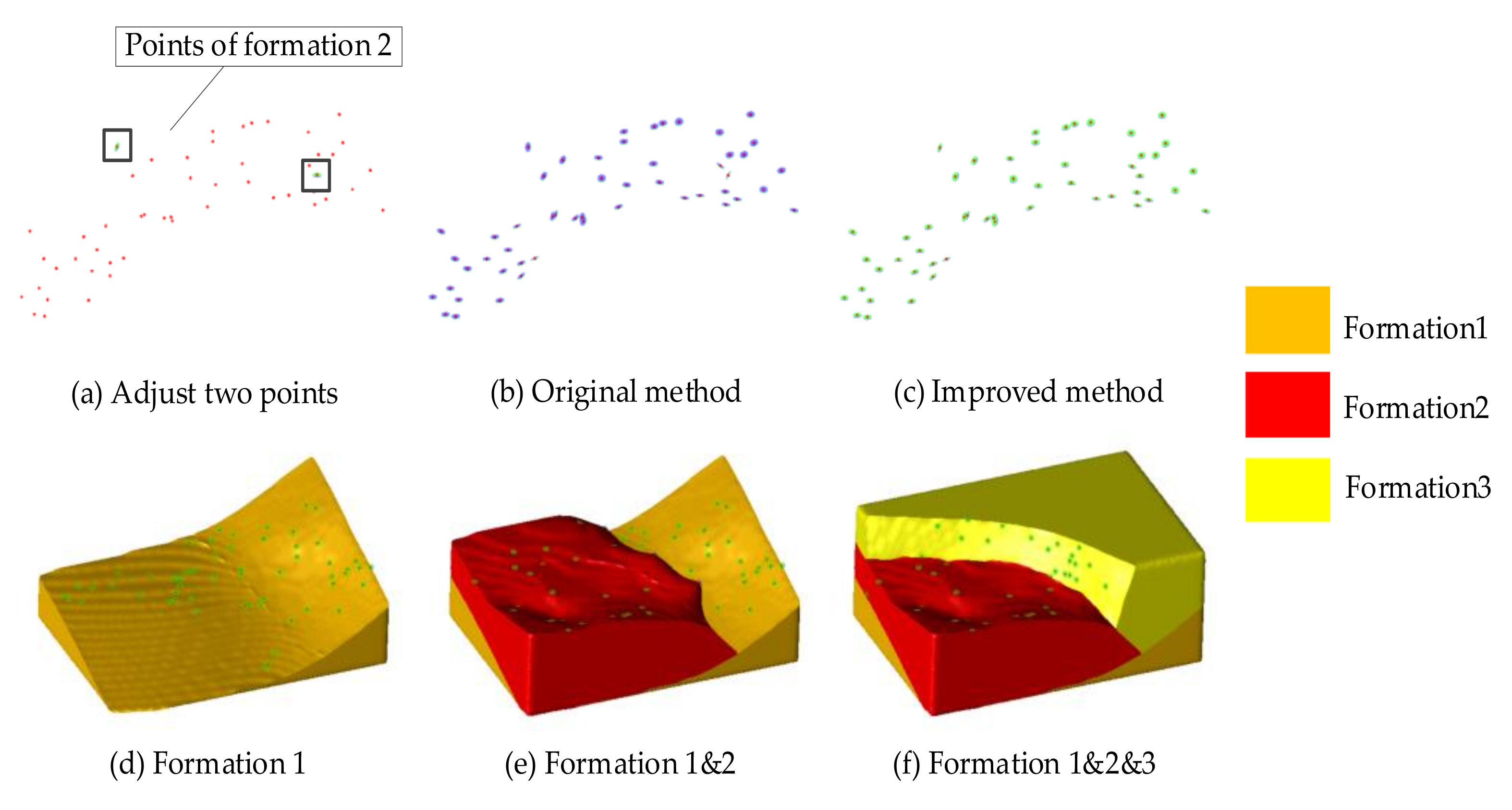
2.3. Implicit Modeling

The main ideas of the implicit modeling method [
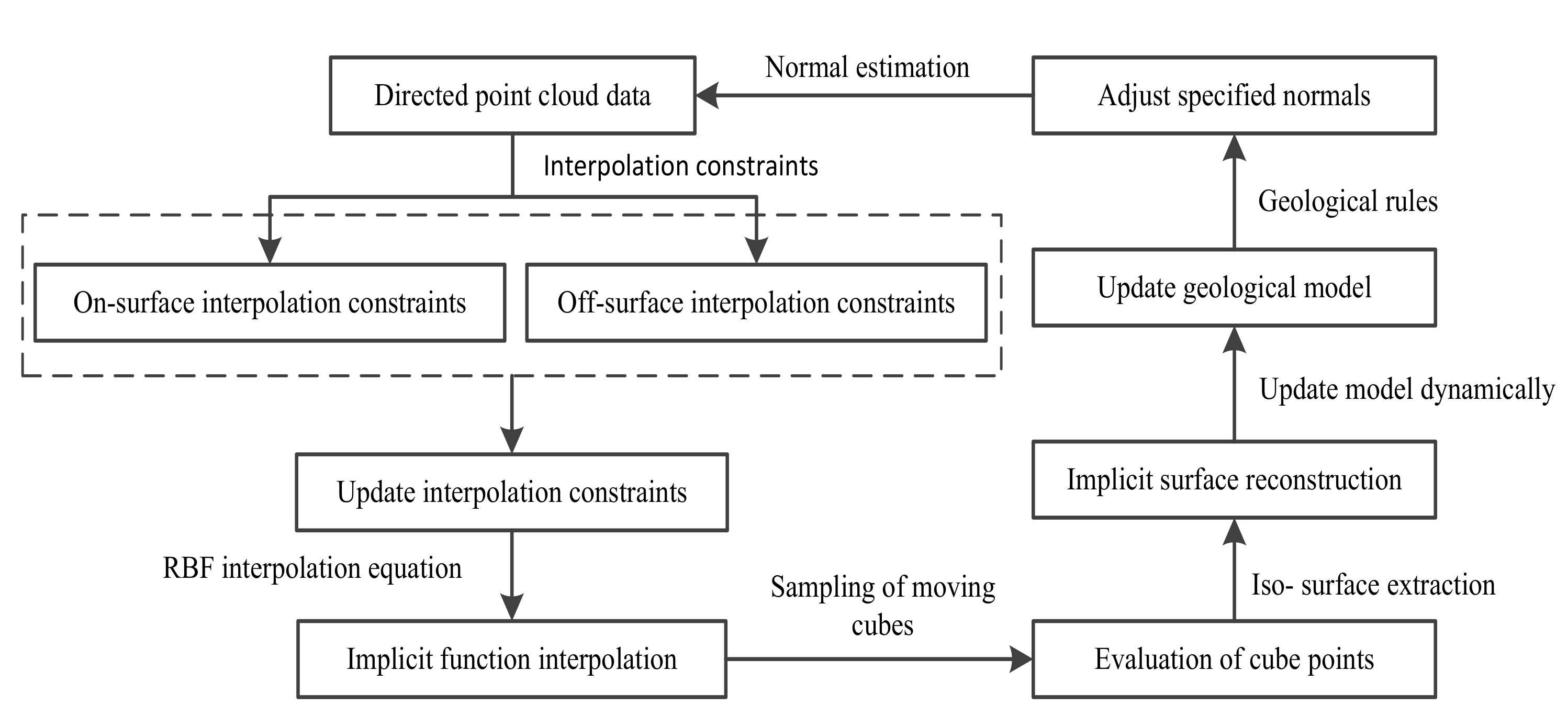
33] of ore body based on geological sampling data are as follows. First, the method uses discretization to convert corresponding types of geological data into interpolation constraints at a certain sampling interval. Second, the method obtains the implicit function that characterizes the geological model by solving the interpolation equation constructed by the interpolation constraint. Finally, the method uses the contour surface extraction method to reconstruct the implicit function that characterizes the geological model. Figure 7 shows the implicit modeling process.
After determining the normal direction of the constraint point, the existing implicit modeling method can be directly used to reconstruct geological model. Considering that the radial basis function interpolation method has superior extrapolation performance, this paper uses the radial basis function to interpolate the constraint points whose normal directions are determined.
The radial basis interpolation function s x has the following form:
s x = s Φ x + p x = j = 1 N ω i Φ x , x j + p x
where x 1 , x 2 , , x N is a set of different interpolation points, and ω i is the weight coefficient to be determined. Φ x , x j is a radial basis kernel function.   s Φ x is the kernel function, and p x is the polynomial.
The radial basis interpolation function s x is usually used for interpolation to satisfy the following constraints.
s x i = f i ,        i = 1 , 2 , N
where f i is the function value at the interpolation point x i .
To interpolate the normal direction of the constraint points, the method of adaptive off-plane constraints can be used to transform the normal constraint into the point constraints. The constraint point x i on the geological surface satisfies the on-surface constraint f x i = 0 . The parameter δ is selected as the offset distance of the constraint point, and the constraint point is offset along its normal direction n i by a distance of δ to obtain the following off-surface constraints.
f x i p o s = + δ f x i n e g = δ
x i p o s = x i + δ n x i n e g = x i δ n
By solving the interpolation equation composed of the above on-surface constraints and off-surface constraints, the radial basis interpolation function s x that represents the geological model can be obtained.
To visualize the radial basis interpolation function s x that implicitly expresses the geological body model, it is necessary to reconstruct the surface of the abstract implicit function according to the needs of the practical applications to obtain a polygonal mesh model. After solving the implicit function, the method of surface reconstruction can be used to obtain geological mesh models with different sizes.

3. Results

This paper tests the proposed method on five data sets. The data sets contain different geological bodies data. Table 1 shows the parameter values of the experimented data sets, including the number of constraint points (NC), the number of neighborhood points in the normal estimation process (N1), and the number of neighborhood points in the normal redirection process (N2).
The sampling points are sparse and uneven, and the original geological bodies are irregular in shape. The angle and color of the circle surrounding the point clouds in the figures represent the normal direction and orientation of the point clouds. The circle surrounding the point clouds is purple; thus, the normal direction of the point is facing the inside of the model, which is the wrong normal direction and needs to be flipped. The circle surrounding the point clouds is green; thus, the normal direction of the point is facing the outside of the model, which is the correct normal direction.
Figure 8 shows the normal estimation results of the first data set. The experiment did not model the first set of data. The model shown in the picture is only a model for reference, and the purpose is to analyze and evaluate the results of normal estimation. Figure 8a,b respectively show the original geological sampling points and the normal estimation result obtained by using the original local plane fitting method. It can be clearly seen that when the original method is used to process sparse and uneven geological sampling points, there are many problems in the normal estimation result. The normal directions of many points are inaccurate and the normals are oriented inside the model, which makes it difficult to meet the requirements of the implicit modeling method. By using the improved method in this paper, after adjusting the normals of certain points manually, the normal estimation results have been significantly improved (Figure 8c–f). The normal orientations of the point clouds are corrected to face the outside of the model, and the normal directions are more accurate. As the number of points with existing normals increases, the result of normal estimation will be more improved.
Figure 9 shows the normal estimation results of the second data set. The model shown in the picture is only a reference model, the purpose is to analyze and evaluate the results of normal estimation. Figure 9a,b respectively show the original geological sampling points and the normal estimation result obtained by using the original local plane fitting method. As the number of the points with existing normals increases, the results of normal estimation become more accurate. After only specifying the normals of two points, the normals of most points are greatly improved compared with the original method. However, as shown in Figure 9b,d, when the normal direction of only one point is adjusted, the normal estimation result obtained by the improved method has errors. Normals with correct orientations in the original method are reversed to the wrong orientations. This is because the improved method in this paper uses the breadth-first search method in the process of normal propagation. The points whose normals have been adjusted will preferentially affect the near points, while the far points will not be affected. Therefore, to obtain more accurate normal estimation result, it is necessary to adjust the normals of points in different regions. In this way, it can be ensured that the normal estimation result of each region is correct.
Figure 10 and Figure 11 show the normal estimation results and geological modeling results of the third and fourth data set. The sampling points shown in the figure belong to Formation 2. In Figure 10, the normal directions of four points have been adjusted manually. In Figure 11, the normal directions of two points have been adjusted manually. The normal estimation results obtained by the improved method are more accurate, and the normal orientations of the point clouds are all toward the outside of the model. Figure 10 and Figure 11 show the multi-layer formation modeling results obtained by using the improved method. Because the original sampling points are sparse and uneven, it is necessary to adjust the normal directions of certain points dynamically and iteratively estimate the normal directions of the point clouds. Therefore, the effect of the point clouds normal estimation can well meet the requirements for implicit geological modeling method.

4. Discussion

Based on the improved normal dynamic estimation method, this paper uses the implicit modeling method to continue the dynamic geological modeling. Because the implicit modeling method relies on the normal estimation method based on local surface fitting, it is suitable for surface reconstruction of smooth geological models. However, it is difficult to process point clouds with a thin surface and sharp surface. In addition, the method proposed in this paper has limitations that need to be improved.
In practical applications, it is found that the normal estimation and normal reorientation process are prone to errors when the geological body has a large distortion or thin surface features. Figure 12 shows the normal estimation results when the geological body has a large distortion or thin surface. It is an inevitable defect of the method based on local plane fitting. Since the method uses the inverse distance weighting when estimating the normal, the point clouds in the large deformation region or thin surface region will have a greater weighting influence on each other’s normal estimation. However, the point clouds in these regions belong to different geological body distributions, and they have little influence on each other. This is an inherent defect of the normal estimation method based on local plane fitting. In addition, the original minimum spanning tree method needs to select the starting point for normal propagation. If the normal of the starting point is toward the inside of the model, the normal direction of the subsequent point cloud will be incorrectly reversed. This is the defect of the original minimum spanning tree method. At present, normal estimation methods based on local plane fitting are still mainly applied to dense point clouds. For sparse and uneven point clouds, the uncertainty of normal estimation is greater. Although the improved method in this paper considers the additional constraints of manually specifying the normal directions in the process of point clouds normal estimation, the method still needs further improvement. Normal estimation and normal redirection should not only consider the spatial position relationship between unorganized point clouds but should also further consider the shape feature constraints of the geological body or the geological rules in the corresponding geological environment. For example, scholars have proposed that the direction constraint of normal propagation can be considered during constructing a Riemann graph in the normal redirection process; thus, the normal propagates along the tangential direction of the surface as much as possible to process geological sampling data with thin surface features.
The size of the geological body and the number of point clouds have no effect on the applicability of the method. The effect of the method is mainly affected by two aspects. One is the neighborhood size of the point cloud; the other is the sparseness and unevenness of the point cloud itself.

5. Conclusions

This paper proposes a geological modeling method based on the normal dynamic estimation of sparse point clouds. The method can be used not only for the normal estimation of sparse point clouds, but also for the normal estimation of dense point clouds. In addition, the method is not only used for modeling of geological bodies, but also for 3D surface reconstruction tasks of general objects. The main innovation of the method is to allow geological engineers to dynamically adjust the normals of certain points and then re-estimate the normals of point clouds. First, this paper improves the point clouds normal estimation method based on local surface fitting. In the normal estimation process, the influence of the points whose normal directions have been adjusted is considered to be the normal direction estimation of the surrounding points, and the influence is added to the objective function as a constraint item. Second, this paper improves the point clouds normal redirection method based on a minimum spanning tree. The improved normal redirection method can automatically select the points with the correct normal directions as the starting points of normal propagation, which overcomes the defects of the original method. By using multiple sets of geological sampling points for verification, the results show that the method proposed in this paper can accurately estimate the normal directions of the sparse and uneven point clouds; thus, the normal direction estimation results can better meet the requirements of implicit modeling.
The method proposed in this paper is still based on the idea of local surface fitting, and the premise of this kind of method is that the local surface of any point in the point clouds can be fitted with a local plane. Therefore, the method proposed in this paper still has certain defects when handling the thin surface region or the region with large distortion. In addition, because the distribution of geological sampling points is not uniform, the number of optimal neighborhood points for fitting a local plane is different for different regions. However, the method proposed in this paper uses a fixed number of neighborhood points for fitting the local plane, which needs to be further improved.

Author Contributions

T.S. and D.Z. designed and performed the experiments. T.S. and D.Z. analyzed the data. T.S. and D.Z. implemented the source code. T.S., D.Z. and L.W. wrote and revised the manuscript. All authors have read and agreed to the published version of the manuscript.

Funding

This work was financially supported by the National Key R&D Program of China (2017YFC0602905).

Institutional Review Board Statement

Not applicable.

Informed Consent Statement

Not applicable.

Data Availability Statement

Not applicable.

Acknowledgments

Thanks to the public datasets used in this research. We also thank the reviewers for their comments and suggestions to improve the quality of the paper.

Conflicts of Interest

The authors declare no competing interest.

References

  1. Barthe, L.; Dodgson, N.A.; Sabin, M.A.; Wyvill, B.; Gaildrat, V. Two-dimensional potential fields for advanced implicit modeling operators. Comput Graph Forum. 2003, 22, 23–33. [Google Scholar] [CrossRef] [Green Version]
  2. Cowan, E.J.; Beatson, R.K.; Ross, H.J.; Fright, W.R.; Titley, M. In Practical implicit geological modelling. In Proceedings of the AusIMM 5th International Mining Geology Conference, Bendigo, Victoria, Australia, 17–19 November 2003; pp. 89–99. [Google Scholar]
  3. Vollgger, S.A.; Cruden, A.R.; Cowan, J.E. In 3d implicit geological modeling of a gold deposit from a structural geologist’s point of view. In Proceedings of the 12th SGA Biennial Meeting—Mineral Deposit Research for a High-Tech World, SGA, Uppsala, Sweden, 12 August 2013; pp. 1–4. [Google Scholar]
  4. Laurent, G.; Aillères, L.; Caumon, G.; Grose, L. Folding and poly-deformation modelling in implicit modelling approach. In Proceedings of the 34th Gocad Meet, Nancy, France, September 2014; pp. 1–18. [Google Scholar]
  5. Renaudeau, J.; Malvesin, E.; Maerten, F.; Caumon, G. Implicit structural modeling by minimization of the bending energy with moving least squares functions. Math. Geosci. 2019, 51, 1–32. [Google Scholar] [CrossRef]
  6. Calcagno, P.; Chilès, J.P.; Courrioux, G.; Guillen, A. Geological modelling from field data and geological knowledge: Part i. Modelling method coupling 3d potential-field interpolation and geological rules. Phys. Earth Planet Inter. 2008, 171, 147–157. [Google Scholar] [CrossRef]
  7. Guillen, A.; Calcagno, P.; Courrioux, G.; Joly, A.; Ledru, P. Geological modelling from field data and geological knowledge: Part ii. Modelling validation using gravity and magnetic data inversion. Phys. Earth Planet Inter. 2008, 171, 158–169. [Google Scholar] [CrossRef]
  8. Hillier, M.J.; Schetselaar, E.M.; de Kemp, E.A.; Perron, G. Three-dimensional modelling of geological surfaces using generalized interpolation with radial basis functions. Math. Geosci. 2014, 46, 931–953. [Google Scholar] [CrossRef]
  9. Grose, L.; Laurent, G.; Aillères, L.; Armit, R.; Jessell, M.; Caumon, G. Structural data constraints for implicit modeling of folds. J. Struct. Geol. 2017, 104, 80–92. [Google Scholar] [CrossRef] [Green Version]
  10. Zhong, D.Y.; Wang, L.G.; Bi, L. Implicit surface reconstruction based on generalized radial basis functions interpolant with distinct constraints. Appl. Math. Model. 2019, 71, 408–420. [Google Scholar] [CrossRef]
  11. Zhong, D.Y.; Zhang, J.; Wang, L.G. Fast implicit surface reconstruction for the radial basis functions interpolant. Appl. Sci. 2019, 9, 5335. [Google Scholar] [CrossRef] [Green Version]
  12. Ohtake, Y.; Belyaev, A.; Alexa, M.; Turk, G.; Seidel, H.P. In Multi-level partition of unity implicits. In Proceedings of the Acm Siggraph 2005 Courses, Los Angeles, CA, USA, 31 July–4 August 2005; pp. 173–180. [Google Scholar]
  13. Kolluri, R. Provably good moving least squares. TALG 2008, 4, 1–25. [Google Scholar] [CrossRef]
  14. Kazhdan, M.; Bolitho, M.; Hoppe, H. In Poisson surface reconstruction. In Proceedings of the fourth Eurographics Symposium on Geometry Processing, Cagliari, Sardinia, Italy, 26–28 June 2006; pp. 61–70. [Google Scholar]
  15. Öztireli, A.C.; Guennebaud, G.; Gross, M. Feature preserving point set surfaces based on non-linear kernel regression. Comput. Graph. Forum. 2009, 28, 493–501. [Google Scholar] [CrossRef] [Green Version]
  16. Hoppe, H.; DeRose, T.; Duchamp, T.; McDonald, J.; Stuetzle, W. Surface Reconstruction from Unorganized Points. In Proceedings of the 19th Annual Conference on Computer Graphics and Interactive Techniques, New York, NY, USA, 1 July 1992; pp. 71–78. [Google Scholar]
  17. Gross, M.; Pfister, H. Point-Based Graphics; The Morgan Kaufmann Series in Computer Graphics; Morgan Kaufmann Publishers Inc.: San Francisco, CA, USA, 2007. [Google Scholar]
  18. Gross, M.; Keiser, R.; Kobbelt, L.P.; Pauly, M. Shape modeling with point-sampled geometry. TOG 2003, 22, 641–650. [Google Scholar]
  19. Lalonde, J.F.; Unnikrishnan, R.; Vandapel, N.; Hebert, M. Scale selection for classification of point-sampled 3-d surfaces. In Proceedings of the Fifth International Conference on 3-D Digital Imaging and Modeling, Ottawa, ON, Canada, 13–16 June 2005; pp. 285–292. [Google Scholar]
  20. Mitra, N.J.; Nguyen, A.; Guibas, L. Estimating surface normals in noisy point clouds data. Int. J. Comput. Geom. Appl. 2004, 14, 261–276. [Google Scholar] [CrossRef]
  21. Amenta, N.; Bern, M. Surface Reconstruction by Voronoi Filtering. Discrete Comput Geom. 1999, 22, 481–504. [Google Scholar] [CrossRef] [Green Version]
  22. Dey, T.K.; Goswami, S. Provable surface reconstruction from noisy samples. Comput. Geom. 2006, 35, 124–141. [Google Scholar] [CrossRef] [Green Version]
  23. Alliez, P.; Cohen-Steiner, D.; Tong, Y.; Desbrun, M. Voronoi-based variational reconstruction of unoriented point sets. In Proceedings of the Symposium on Geometry Processing, Barcelona, Spain, 4–6 July 2007; pp. 39–48. [Google Scholar]
  24. Rousseeuw, P.J.; Leroy, A.M. Robust Regression and Outlier Detection; John Wiley & Sons, Inc.: New York, NY, USA, 1987. [Google Scholar]
  25. Fleishman, S.; Cohen-Or, D.; Silva., C.T. Robust moving least-squares fitting with sharp features. TOG 2005, 24, 544–552. [Google Scholar] [CrossRef]
  26. Li, B.; Schnabel, R.; Klein, R.; Cheng, Z.Q.; Dang, G.; Jin, S.Y. Robust normal estimation for point clouds with sharp features. Comput. Graph. 2010, 34, 94–106. [Google Scholar] [CrossRef]
  27. Carr, J.C.; Beatson, R.K.; Cherrie, J.B.; Mitchell, T.J.; Fright, W.R.; McCallum, B.C.; Evans, T.R. Reconstruction and representation of 3d objects with radial basis functions. In Proceedings of the 28th Annual Conference on Computer Graphics and Interactive Techniques, Los Angeles, CA, USA, 12–17 August 2001; pp. 67–76. [Google Scholar]
  28. Lorensen, W.E.; Cline, H.E. Marching cubes: A high resolution 3d surface construction algorithm. ACM SIGGRAPH Comput. Graph. 1987, 21, 163–169. [Google Scholar] [CrossRef]
  29. Newman, T.S.; Yi, H. A survey of the marching cubes algorithm. Comput. Graph. 2006, 30, 854–879. [Google Scholar] [CrossRef]
  30. Wu, Z.; Sullivan Jr, J.M. Multiple material marching cubes algorithm. Int. J. Numer. Methods Eng. 2003, 58, 189–207. [Google Scholar] [CrossRef]
  31. Guennebaud, G.; Gross, M. Algebraic point set surfaces. In Proceedings of the Special Interest Group on Computer Graphics and Interactive Techniques Conference, San Diego, CA, USA, 5–9 August 2007; pp. 23–31. [Google Scholar]
  32. Huang, H.; Li, D.; Zhang, H.; Ascher, U.; Cohen-Or, D. Consolidation of unorganized point clouds for surface reconstruction. TOG 2009, 28, 1–7. [Google Scholar] [CrossRef] [Green Version]
  33. Zhong, D.Y.; Wang, L.G.; Bi, L.; Jia, M.T. Implicit modeling of complex orebody with constraints of geological rules. T. Nonferr. Metal. Soc. 2019, 29, 2392–2399. [Google Scholar] [CrossRef]
Figure 1. Overall flow chart of the method.
Mathematics 09 01819 g001
Figure 2. Considering the points whose normals have been adjusted manually.
Mathematics 09 01819 g002
Figure 3. The improved minimum spanning tree method.
Mathematics 09 01819 g003
Figure 4. Union-find sets: (a) the virtual tree; (b) the array used to find node information.
Mathematics 09 01819 g004
Figure 5. The improved minimum spanning tree.
Mathematics 09 01819 g005
Figure 6. The subtrees used for normal propagation.
Mathematics 09 01819 g006
Figure 7. The process of implicit modeling based on the normal dynamic estimation method.
Mathematics 09 01819 g007
Figure 8. Normal estimation results of the first data set. (a,b) show the original sampling points and the normal estimation result obtained by the original method. (c,d) show the normal estimation result obtained after adjusting the normal of only one point. (e,f) show the normal estimation result obtained after adjusting the normals of two points.
Mathematics 09 01819 g008
Figure 9. Normal estimation results of the second data set. (a,b) show the original sampling points and the normal estimation result obtained by the original method. (c,d) show the normal estimation result obtained after adjusting the normal of only one point. (e,f) show the normal estimation result obtained after adjusting the normals of two points.
Mathematics 09 01819 g009
Figure 10. Normal estimation and modeling results of the third data set. (a) shows that the normal directions of the four points have been adjusted artificially. (b) is the normal estimation result obtained by using the original method. (c) is the normal estimation result obtained by using improved method in this paper. (df) show the geological modeling results obtained by using modeling method in this paper.
Mathematics 09 01819 g010
Figure 11. Normal estimation and modeling results of the fourth data set. (a) shows that the normal directions of the two points have been adjusted artificially. (b) is the normal estimation result obtained by using the original method. (c) is the normal estimation result obtained by using improved method in this paper. (df) shows the geological modeling results obtained by using modeling method in this paper.
Mathematics 09 01819 g011
Figure 12. Normal estimation results of the fifth data set. (a) shows the original sampling points. (b) shows the normal estimation result obtained using the original method. (c) shows that the normal directions of the three points have been adjusted artificially. (d) shows the normal estimation result obtained by using the improved method, in which the black box area represents the large distortion and thin surface.
Mathematics 09 01819 g012
Table 1. Parameter values of the experimented data sets.
Data SetsNCN1N2
123655
220055
317155
417155
550455
Publisher’s Note: MDPI stays neutral with regard to jurisdictional claims in published maps and institutional affiliations.

