On the Implicit Equation of Conics and Quadrics Offsets

Abstract

A new determinantal representation for the implicit equation of offsets to conics and quadrics is derived. It is simple, free of extraneous components and provides a very compact expanded form, these representations being very useful when dealing with geometric queries about offsets such as point positioning or solving intersection purposes. It is based on several classical results in “A Treatise on the Analytic Geometry of Three Dimensions” by G. Salmon for offsets to non-degenerate conics and central quadrics.

1. Introduction

Let $\delta >0$ be a fixed real number. Given a curve $\mathcal{C}$ in ${\mathbb{R}}^2$ or a surface $\mathcal{S}$ in ${\mathbb{R}}^3$, their respective $\delta$-offset, denoted by ${\mathcal{C}}_{\delta }$ and ${\mathcal{S}}_{\delta }$, is the locus of the points that are at constant Euclidean distance $\delta$, measured along the normal line, from the curve $\mathcal{C}$ or surface $\mathcal{S}$.

Offsets have a variety of useful applications in computer-aided design, such as tool path control, geometric modeling, NC milling, design of surfaces with homogeneous thickness and tolerance analysis in manufacturing (see, for example, Ref. [1,2]). This leads to the fact that they have been widely studied by several authors; see, for example, Ref. [3,4,5,6,7,8,9,10]. Moreover, the notion of offset has been generalized in different ways, as reflected in [11,12,13]. Dealing with offset curves is easier when the arc-length of the given curve is polynomial. Thus, Pythagorean hodograph (PH) curves, spatial PH curves, rational PH curves and Minkowski PH curves have been thoroughly studied (see [14,15,16] and the bibliography in [13]). Regarding surfaces, Pythagorean normal (PN) surfaces were introduced by Pottmann [17].

It is well known that the offset of a rational curve $\mathcal{C}$ or a rational surface $\mathcal{S}$ is an algebraic curve or surface, but it is not rational in most cases. In fact, there are numerous articles where conditions for curves and surfaces are studied so that their offsets are rational (see, for example, [18,19,20,21]). In addition, the implicit equation of the offset is typically of much higher degree than the initial curve or surface, has many terms and coefficients of large size and its calculation involves using elimination methods that are not always effective.

However, G. Salmon proved in his classical texts [22,23] that the implicit equation of the offset to non-degenerate conics and to central quadrics can be characterized in terms of the discriminant of a univariate polynomial. We show here that this representation works for the implicit equation of ${\mathcal{C}}_{\delta }$ and ${\mathcal{S}}_{\delta }$ when $\mathcal{C}$ is any conic and $\mathcal{S}$ is any quadric. These implicit equations are of determinantal type and free of extraneous components; they provide a very compact expanded form and they are very useful when dealing with geometric queries such as point positioning for offsets or solving intersection purposes involving offsets. This is one of the main motivations for deriving these new representations for the offset implicit equations that can be considered a complement to the new lower-degree rational parametrizations of regular quadric offsets introduced in [18] when manipulating offsets to quadrics. Finally, we should mention that in [24], a determinantal form for the implicit equation for offsets to non-degenerate conics and quadrics was introduced. Here, we refine these formulas, analyze the degenerate cases, provide explicit proofs and include more applications.

This paper is divided into six sections. Following this introduction, the second section introduces the usual formula defining offsets to plane curves and surfaces. In the third one, the implicit equation of the offset to a conic is presented as the determinant of a $4\times 4$ or a $3\times 3$ matrix, the proof being fully computational. The fourth one introduces the implicit equation of the offset to a quadric as the determinant of a $6\times 6$ or a $4\times 4$ matrix, the proof being fully computational too. The fifth section shows some geometric queries involving offsets to quadrics where the introduced implicit equations are used. The last section is devoted to the conclusions of the paper.

2. Preliminaries

The next subsections provide some basic notions and the equations describing the offsets to curves and surfaces.

2.1. Conics and Quadrics Representation

Let $\mathcal{A}$ be a conic in ${\mathbb{R}}^2$. Let $\mathcal{X}=(X,Y,1)$. It is well known that the implicit equation of $\mathcal{A}$ in ${\mathbb{R}}^2$ can be written as

$$a(X,Y)=a_{11}{X}^2+a_{22}{Y}^2+2a_{12}XY+2a_{13}X+2a_{23}Y+a_{33}=0,$$

or in matricial form $\mathcal{A}:\mathcal{X}A{\mathcal{X}}^t=0$, where A is the symmetric matrix

$$A=\left(\begin{array}{ccc}{a}_{11}& a_{12}& a_{13}\\ a_{12}& a_{22}& a_{23}\\ a_{13}& a_{23}& a_{33}\end{array}\right).$$

Continuing in the same way, let $\mathcal{A}$ be a quadric in ${\mathbb{R}}^3$ and $\mathcal{X}=(X,Y,Z,1)$. The implicit equation of a quadric $\mathcal{A}$ in ${\mathbb{R}}^3$ can be written as

$$\begin{array}{c}\hfill a(X,Y,Z)=a_{11}{X}^2+a_{22}{Y}^2+a_{33}{Z}^2+2a_{12}XY+2a_{13}XZ+2a_{23}YZ\\ \hfill +2a_{14}X+2a_{24}Y+2a_{34}Z+a_{44}=0,\end{array}$$

or in matricial form $\mathcal{A}:\mathcal{X}A{\mathcal{X}}^t=0$, where $\mathcal{X}=(X,Y,Z,1)$ and A is the symmetric matrix

$$A=\left(\begin{array}{cccc}{a}_{11}& a_{12}& a_{13}& a_{14}\\ a_{12}& a_{22}& a_{23}& a_{24}\\ a_{13}& a_{23}& a_{33}& a_{34}\\ a_{14}& a_{24}& a_{34}& a_{44}\end{array}\right).$$

2.2. Describing the Implicit Equation of an Offset

Given a curve $\mathcal{C}$ in ${\mathbb{R}}^2$, the $\delta$-offset to $\mathcal{C}$, ${\mathcal{C}}_{\delta }$, is the locus of the points in ${\mathbb{R}}^2$, which are at constant Euclidean distance $\delta$ from the initial curve $\mathcal{C}$ along its normal line. The offset of a curve is generally not rational (even when $\mathcal{C}$ is rational) but it is always an algebraic curve. The implicit equation of the $\delta$-offset ${\mathcal{C}}_{\delta }$ is usually a very dense polynomial of higher degree than the one of the original curve. If the curve $\mathcal{C}$ is presented by its implicit equation $f(x,y)=0$, then the computation of the implicit equation of ${\mathcal{C}}_{\delta }$ requires the elimination of $\alpha$ and $\beta$ from these three equations:

$$f(\alpha ,\beta )=0,{(x-\alpha )}^2+{(y-\beta )}^2-{\delta }^2=0,(x-\alpha )f_y(\alpha ,\beta )-(y-\beta )f_x(\alpha ,\beta )=0.$$

Similarly, given a surface $\mathcal{S}$ in ${\mathbb{R}}^3$, the $\delta$-offset to $\mathcal{S}$, ${\mathcal{S}}_{\delta }$, is the locus of the points in ${\mathbb{R}}^3$, which are at constant Euclidean distance $\delta$ from the initial surface $\mathcal{S}$ (along its normal line). As in the case of curves, ${\mathcal{S}}_{\delta }$ is generally not rational. If the surface $\mathcal{S}$ is given by its implicit equation $f(x,y,z)=0$, then the computation of the implicit equation of ${\mathcal{S}}_{\delta }$ requires the elimination of $\alpha$, $\beta$ and $\gamma$ from these four equations:

$$\begin{array}{c}\hfill f(\alpha ,\beta ,\gamma )=0,\\ \hfill (x-\alpha )f_y(\alpha ,\beta ,\gamma )-(y-\beta )f_x(\alpha ,\beta ,\gamma )=0,\\ \hfill {(x-\alpha )}^2+{(y-\beta )}^2+{(z-\gamma )}^2-{\delta }^2=0,\\ \hfill (y-\beta )f_z(\alpha ,\beta ,\gamma )-(z-\gamma )f_y(\alpha ,\beta ,\gamma )=0.\end{array}$$

Consequently, the implicit equation of offsets can be obtained using elimination techniques but this can be a time-consuming calculation and, even so, we do not always obtain a closed formula without extraneous factors.

2.3. Discriminant of a Polynomial

Let $f\left(x\right)$ and $g\left(x\right)$ be two univariate polynomials with coefficients in a field:

$$f\left(x\right)=\sum _{i=0}^m{a}_i{x}^i,g\left(x\right)=\sum _{i=0}^n{b}_i{x}^i.$$

Then, the Sylvester matrix of $f\left(x\right)$ and $g\left(x\right)$ with respect to x, denoted by $\mathrm{Syl}(f,g,x)$, is defined as

$$\mathrm{Syl}(f,g,x)=\stackrel{n+m}{\overbrace{\left(\begin{array}{c}\begin{array}{ccc}{a}_m& \dots & a_0\\ & \ddots & & \ddots & \\ & & a_m& \dots & a_0\end{array}\\ \begin{array}{ccc}{b}_n& \dots & b_0\\ & \ddots & & \ddots & \\ & & b_n& \dots & b_0\end{array}\end{array}\right)}}\begin{array}{cc}\left.\begin{array}{c}\\ \\ \end{array}\right\}& n\\ \left.\begin{array}{c}\\ \\ \end{array}\right\}& m\end{array}.$$

The resultant of $f\left(x\right)$ and $g\left(x\right)$ with respect to x, denoted by $\mathrm{Res}(f,g,x)$, is the determinant of the Sylvester matrix. It is well known that $\mathrm{Res}(f,g,x)=0$ if and only if $f\left(x\right)$ and $g\left(x\right)$ have a common nontrivial factor. Moreover, the discriminant of $f\left(x\right)$ is defined to be

$$\mathrm{disc}\left(f\right)={\displaystyle \frac{{(-1)}^{\frac{m(m-1)}{2}}}{a_m}}\mathrm{Res}(f,f^{\prime },x),$$

and it is widely known that $f\left(x\right)$ has a multiple root if and only if its discriminant vanishes.

3. On the Implicit Equation for the $\mathbf{\delta }$-Offset to a Conic

Given two conics $\mathcal{A}:\mathcal{X}A{\mathcal{X}}^t=0$ and $\mathcal{B}:\mathcal{X}B{\mathcal{X}}^t=0$, their characteristic equation is defined as

$$f(\lambda )=det(\lambda B+A)=det\left(B\right){\lambda }^3+\dots +det\left(A\right).$$

From now on, in this section, we will assume that $\mathcal{B}:\mathcal{X}B{\mathcal{X}}^t=0$ is a circle with center $(x,y)$, radius $\delta$ and

$$B=\left(\begin{array}{ccc}1& 0& -x\\ 0& 1& -y\\ -x& -y& x^2+y^2-{\delta }^2\end{array}\right).$$

In this case, the characteristic polynomial of a conic $\mathcal{A}$ and a circle $\mathcal{B}$ is a cubic polynomial in $\lambda$ since $det\left(B\right)=-{\delta }^2\ne 0$. More precisely, if

$$f(\lambda )=det(\lambda B+A)\stackrel{\mathrm{def}}{=}-{\delta }^2{\lambda }^3+e_2(x,y){\lambda }^2+e_1(x,y)\lambda +det\left(A\right),$$

(1)

we have that

$$\begin{array}{ccc}\hfill e_2(x,y)& =& a(x,y)-{\delta }^2(a_{11}+a_{22}),\hfill \\ \hfill e_1(x,y)& =& \left(a_{11}{a}_{22}-a_{12}^2\right)\left(x^2+y^2-{\delta }^2\right)+2\left(a_{13}{a}_{22}-a_{12}{a}_{23}\right)x\hfill \\ & & +2\left(a_{11}{a}_{23}-a_{12}{a}_{13}\right)y+a_{11}{a}_{33}-a_{13}^2+a_{22}{a}_{33}-a_{23}^2=\hfill \\ & =& \left|\begin{array}{cc}{a}_{11}& a_{12}\\ a_{12}& a_{22}\end{array}\right|\left(x^2+y^2-{\delta }^2\right)+2\left|\begin{array}{cc}{a}_{13}& a_{12}\\ a_{23}& a_{22}\end{array}\right|x+2\left|\begin{array}{cc}{a}_{11}& a_{13}\\ a_{12}& a_{23}\end{array}\right|y\hfill \\ & & +\left|\begin{array}{cc}{a}_{11}& a_{13}\\ a_{13}& a_{33}\end{array}\right|+\left|\begin{array}{cc}{a}_{22}& a_{23}\\ a_{23}& a_{33}\end{array}\right|\hfill \end{array}$$

with ${deg}_{x,y}{e}_i(x,y)=2$.

We say that two conics are touching each other when they intersect in a point with the same tangent line. The following result can be found in [23].

Theorem 1

(see [23]). Given a non-degenerate conic and a circle, they touch each other if and only if their characteristic equation has a multiple root.

Next, we observe that the center $(x,y)$ of a circle belongs to the offset to the conic $\mathcal{A}$ to distance $\delta$ if and only if $\mathcal{A}$ is tangent to $\mathcal{B}$. This implies that they touch each other and then, according to the previous theorem, the discriminant of $f(\lambda )$ must vanish. Moreover, the next theorem shows that not only the discriminant must vanish but it is equal to the implicit equation of the offset.

Theorem 2.

Let δ be a positive real number and let $\mathcal{A}$ be a non-degenerate conic different from a circle. The implicit equation of ${\mathcal{A}}_{\delta }$, $a_{\delta }(x,y)$, agrees with the discriminant (with respect to λ) of the characteristic equation of $\mathcal{A}$ and the circle of radius δ and center $(x,y)$.

Proof. 

A point $(x_0,y_0)$ is on its offset ${\mathcal{A}}_{\delta }$ if there exists another point $(X_0,Y_0)$ with

$$\mathcal{A}(X_0,Y_0)=\mathcal{B}(X_0,Y_0)=0,$$

where $\mathcal{B}$ equals the circle of radius $\delta$ and center $(x_0,y_0)$, such that the tangent vectors to $\mathcal{A}$ and $\mathcal{B}$ at the point $(X_0,Y_0)$ are proportional. This implies that the Jacobian determinant

$$D(X,Y)\stackrel{\mathrm{def}}{=}\left|{\displaystyle \frac{\partial (\mathcal{A},\mathcal{B})}{\partial (X,Y)}}\right|$$

must vanish at $(X_0,Y_0,x_0,y_0)$. Thus, one way to obtain the implicit equation of ${\mathcal{A}}_{\delta }$ is simply to eliminate the variables $(X,Y)$ from the equations

$$\mathcal{A}(X,Y)=0,\mathcal{B}(X,Y)=0,D(X,Y)=0.$$

Assume that our conic $\mathcal{A}$ is written in canonical form (see Remark 1). If $A=\mathrm{diag}(a_{11},a_{22},a_{33})$, then

$$D=\left|\begin{array}{cc}2{\mathit{a}}_{\mathit{11}}X& 2a_{22}Y\\ 2X-2\mathit{x}& 2Y-2\mathit{y}\end{array}\right|=4((a_{11}-a_{22})XY-a_{11}X\mathit{y}+a_{22}Y\mathit{x})=4\mathcal{D}(X,Y).$$

Eliminating $(X,Y)$ from $\mathcal{A}(X,Y)=0,\mathcal{B}(X,Y)=0,\mathcal{D}(X,Y)=0$ by performing the next steps,

$$f_1=\mathrm{resultant}(\mathcal{D},\mathcal{B},Y),f_2=\mathrm{resultant}(\mathcal{D},\mathcal{A},Y),f_3=\mathrm{resultant}(f_1,f_2,X)),$$

we obtain

$$f_3(x,y)=a_{11}^4{a}_{22}^4{x}^4{y}^4{(a_{11}-a_{22})}^6\mathrm{discrim}\left(f(\lambda )\right).$$

Observe now that if $\mathcal{A}$ represents either an ellipse or a hyperbola, then the axes $x=0$ and $y=0$ do not belong to the offset. Moreover, $a_{11}^4{a}_{22}^4{(a_{11}-a_{22})}^6\ne 0$ and, therefore, we can conclude that the implicit equation is the discriminant.

If A defines a parabola, $x^2=2py,p\ne 0$, proceeding in the same way, it is found that $f_3(x,y)=p^2{x}^2\mathrm{discrim}\left(f(\lambda )\right)$ and the implicit equation agrees with the discriminant too.   □

Remark 1.

If the conic is not presented in canonical form, then there exists a rigid motion of the plane of matrix P, with $P^{-1}=L$, that makes the axes of the transformed conic $\tilde{\mathcal{A}}=P\left(\mathcal{A}\right)$ of matrix $\tilde{A}=L^{T}AL$ to be $x^{\prime }=0$ and $y^{\prime }=0$, with $P(x,y)=(x^{\prime },y^{\prime })$. Hence, the implicit equation of the δ–offset to $\tilde{\mathcal{A}}$, as we have seen in the proof of Theorem 2, is the λ-discriminant of $\tilde{f}(\lambda ,x^{\prime },y^{\prime })=det(\lambda \tilde{B}+L^{T}AL)$, where $\tilde{B}$ is the matrix of the circle $\tilde{\mathcal{B}}$ of center $(x^{\prime },y^{\prime })$ and radius δ. On the other hand, a point $(x,y)$ lies in the δ-offset of $\mathcal{A}$ if and only if $P(x,y)$ lies in the δ-offset of $\tilde{\mathcal{A}}$. Therefore, the implicit equation of the δ-offset of $\mathcal{A}$ must be the λ-discriminant of $\tilde{f}(\lambda ,P(x,y))$. Since the transformed circle $\tilde{\mathcal{B}}=P\left(\mathcal{B}\right)$, of center $P(x,y)$ and radius δ, has matrix $L^{T}BL$, where B is the matrix of the circle $\mathcal{B}$ of center $(x,y)$ and radius δ, we have

$$\tilde{f}(\lambda ,P(x,y)))=det(\lambda L^{T}BL+L^{T}AL)=det\left(L^T(\lambda B+A)L\right)=det{\left(L\right)}^{2}f(\lambda ,x,y).$$

Since L is a rigid motion, the principal $2\times 2$ minor is an orthogonal matrix and the last row is $(0,0,1)$, so $det\left(L\right)=\pm 1$, so the λ-discriminant of $f(\lambda ,x,y)$ and $\tilde{f}(\lambda ,P(x,y))$ agree, so the assumption on the canonical form in the proof of Theorem 2 can be assumed without loss of generality.

The following lemma expresses the discriminant of the characteristic equation of $\mathcal{A}$ and the circle of radius $\delta$ and center $(x,y)$ in a compact way in terms of the polynomials $e_1(x,y)$ and $e_2(x,y)$ presented in (1).

Lemma 1.

Given a conic $\mathcal{A}$ and a circle, the discriminant of its characteristic equation is given by

$$\mathrm{discrim}\left(f(\lambda )\right)=\left|\begin{array}{cccc}{\delta }^2& 0& e_1(x,y)& 2det\left(A\right)\\ e_2(x,y)& 2e_1(x,y)& 3det\left(A\right)& 0\\ 0& e_2(x,y)& 2e_1(x,y)& 3det\left(A\right)\\ 0& -3{\delta }^2& 2e_2(x,y)& e_1(x,y)\end{array}\right|.$$

(2)

Proof. 

The discriminant of $f(\lambda )$ is by definition equal to the resultant of $f(\lambda )$ and $f^{\prime }(\lambda )$ divided by ${\delta }^2$. If we perform the convenient row operations on the Sylvester matrix of $f(\lambda )$ and $f^{\prime }(\lambda )$, then we obtain (2).   □

We have the following corollary of Lemma 1 and Theorem 2.

Corollary 1.

Given a non-degenerate conic $\mathcal{A}$, the implicit equation of ${\mathcal{A}}_{\delta }$, $a_{\delta }(x,y)$, is given by

$$\begin{array}{ccc}{a}_{\delta }(x,y)\hfill & =\hfill & \left|\begin{array}{cccc}{\delta }^2& 0& e_1(x,y)& 2det\left(A\right)\\ e_2(x,y)& 2e_1(x,y)& 3det\left(A\right)& 0\\ 0& e_2(x,y)& 2e_1(x,y)& 3det\left(A\right)\\ 0& -3{\delta }^2& 2e_2(x,y)& e_1(x,y)\end{array}\right|\hfill \\ \hfill & =\hfill & {\left(e_1(x,y)e_2(x,y)\right)}^2+4{\delta }^2{e}_1^3(x,y)-4det\left(A\right)e_2^3(x,y)\hfill \\ \hfill & & -18{\delta }^{2}det\left(A\right)e_1(x,y)e_2(x,y)-27{\delta }^{4}det{\left(A\right)}^2.\hfill \end{array}$$

The next corollaries show smaller matrices providing the implicit equation of the offset for a non-degenerate conic but with higher-degree entries (and one of them is symmetric). They come from different representations of the resultant in terms of the Bezout matrix (see [25,26]).

Corollary 2.

Given a non-degenerate conic $\mathcal{A}$, the implicit equation of ${\mathcal{A}}_{\delta }$, $a_{\delta }(x,y)$, is given by

$$a_{\delta }(x,y)=\left|\begin{array}{ccc}2e_1& 3{\delta }^{2}det\left(A\right)+e_1{e}_2& 2det\left(A\right)e_2\\ e_2& 2{\delta }^2{e}_1& 3{\delta }^{2}det\left(A\right)\\ 3& 2e_2& e_1\end{array}\right|.$$

Corollary 3.

Given a non-degenerate conic $\mathcal{A}$, the implicit equation of ${\mathcal{A}}_{\delta }$, $a_{\delta }(x,y)$, is given by

$$a_{\delta }(x,y)=\left|\begin{array}{ccc}3& 2e_2& e_1\\ 2e_2& 2e_2^2-2{\delta }^2{e}_1& e_1{e}_2-3{\delta }^{2}det\left(A\right)\\ e_1& e_1{e}_2-3{\delta }^{2}det\left(A\right)& e_1^2-2det\left(A\right)e_2\end{array}\right|.$$

Offsets to Degenerate Conics

The above results require a slight modification when considering degenerate conics. Consider, for example, $a(X,Y)=Y^2$. In this case, $f(\lambda )=-{\delta }^2{\lambda }^3-({\delta }^2-y^2){\lambda }^2$ has $\lambda =0$ as a double root and so the discriminant is identically zero. This gives a counterexample for Theorem 1.

On the other hand, applying the determinantal representation (2), when $det\left(A\right)=0$, it is easy to see that the discriminant factors in the following way:

$$\mathrm{discrim}\left(f(\lambda )\right)=e_1^2(x,y)\left(e_2^2(x,y)+4{\delta }^2{e}_1(x,y)\right),$$

and this polynomial is a multiple of the implicit equation of the offset. Our next result shows that this problem is easily solved by dividing $f(\lambda )$ by $\lambda$.

Lemma 2.

Given a degenerate conic $\mathcal{A}$ and a circle, the discriminant of its characteristic equation divided by λ is equal to

$$\mathrm{discrim}\left({\displaystyle \frac{f(\lambda )}{\lambda }}\right)=e_2^2(x,y)+4{\delta }^2{e}_1(x,y).$$

Proof. 

Using the notation of (1),

$$F(\lambda )\stackrel{\mathrm{def}}{=}{\displaystyle \frac{f(\lambda )}{\lambda }}=-{\delta }^2{\lambda }^2+e_2(x,y)\lambda +e_1(x,y).$$

Using convenient row operations on the Sylvester matrix of $F(\lambda )$ and $F^{\prime }(\lambda )$, we obtain

$$\mathrm{discrim}\left(F(\lambda )\right)=\left|\begin{array}{cc}{e}_2& 2e_1\\ -2{\delta }^2& e_2\end{array}\right|=e_2^2(x,y)+4{\delta }^2{e}_1(x,y),$$

as desired.   □

Thus, we can generalize Theorem 2 to the case when $\mathcal{A}$ is degenerate as follows.

Theorem 3.

Let δ be a positive real number and let $\mathcal{A}$ be a degenerate conic. Let $f(\lambda )$ denote the characteristic equation of $\mathcal{A}$ and the circle of radius δ and center $(x,y)$. Then, the implicit equation of ${\mathcal{A}}_{\delta }$, $a_{\delta }(x,y)$, agrees with the discriminant of $f(\lambda )/\lambda$.

Proof. 

We will apply the same arguments used in Theorem 2, and assume that our conic $\mathcal{A}$ is written in canonical form. Let

$$F(\lambda )={\displaystyle \frac{f(\lambda )}{\lambda }}\mathrm{and}D(X,Y)=\left|{\displaystyle \frac{\partial (\mathcal{A},\mathcal{B})}{\partial (X,Y)}}\right|.$$

If A defines two parallel lines, that is, $A=\mathrm{diag}(0,a_{22},a_{33})$ with $a_{22}{a}_{33}\ne 0$, then $D=-4a_{22}Y(X-x)=-4\mathcal{D}(X,Y)$. Eliminating $(X,Y)$ from $\mathcal{A}(X,Y)=0,\mathcal{B}(X,Y)=0,\mathcal{D}(X,Y)=0$ by performing the following steps:

$$f_1=\mathrm{resultant}(\mathcal{D},\mathcal{B},X),f_2=\mathrm{resultant}(\mathcal{D},\mathcal{A},X),f_3=\mathrm{resultant}(f_1,f_2,Y)),$$

we obtain

$$f_3(x,y)=a_{22}^4{a}_{33}^2\mathrm{discrim}\left(F(\lambda )\right).$$

Since $a_{22}{a}_{33}\ne 0$, we can conclude that the implicit equation is the discriminant.

If A defines two intersecting lines, that is, $A=\mathrm{diag}(a_{11},a_{22},0)$ with $a_{11}{a}_{22}\ne 0$, then $D=4\left(-XY+Xy\right)a_{11}+\left(XY-xY\right)a_{22}$. Following the same steps as above, we have

$$f_3(x,y)=a_{11}^6{a}_{22}^6{(a_{11}-a_{22})}^6{x}^4{y}^4{({\delta }^2-x^2-y^2)}^2\mathrm{discrim}\left(F(\lambda )\right).$$

Since $\mathcal{A}$ consists of two lines which intersect at the origin, neither the $x,y$-axes nor the circle of radius $\delta$ centered at the origin belong to the offset. Moreover, $a_{11}{a}_{22}\ne 0$ and, therefore, the implicit equation is the discriminant.

If A defines a double line, i.e., $y^2=0$, the discriminant of $F(\lambda )$ is equal to ${\left({\delta }^2-y^2\right)}^2$, which is obviously the equation of the offset.   □

We can conclude that the offset of a degenerate conic is defined by the equation

$$e_2^2(x,y)+4{\delta }^2{e}_1(x,y)=0,$$

its implicit equation being obtained by simply removing multiple factors.

4. On the Implicit Equation for the $\mathbf{\delta }$–Offset to a Quadric

Given two quadrics $\mathcal{A}:\mathcal{X}A{\mathcal{X}}^t=0$ and $\mathcal{B}:\mathcal{X}B{\mathcal{X}}^t=0$, their characteristic equation is defined as

$$f(\lambda )=det(\lambda B+A)=det\left(B\right){\lambda }^4+\dots +det\left(A\right).$$

From now on, in this section, we will assume that $\mathcal{B}:\mathcal{X}B{\mathcal{X}}^t=0$ is the sphere with center $(x,y,z)$, radius $\delta$ and

$$B=\left(\begin{array}{cccc}1& 0& 0& -x\\ 0& 1& 0& -y\\ 0& 0& 1& -z\\ -x& -y& -z& x^2+y^2+z^2-{\delta }^2\end{array}\right).$$

Observe that the characteristic polynomial of a quadric $\mathcal{A}$ and a sphere $\mathcal{B}$ is a quartic polynomial in $\lambda$ since $det\left(B\right)=-{\delta }^2\ne 0$. If

$$f(\lambda )=-{\delta }^2{\lambda }^4+e_3(x,y,z){\lambda }^3+e_2(x,y,z){\lambda }^2+e_1(x,y,z)\lambda +det\left(A\right),$$

(3)

then we have

$$\begin{array}{ccc}\hfill e_3(x,y,z)& =& a(x,y,z)-{\delta }^2(a_{11}+a_{22}+a_{33}),\hfill \\ \hfill e_2(x,y,z)& =& (a_{12}^2+a_{13}^2+a_{23}^2-a_{11}{a}_{22}-a_{11}{a}_{33}-a_{22}{a}_{33}){\delta }^2\hfill \\ & & +(a_{11}{a}_{22}+a_{11}{a}_{33}-a_{12}^2-a_{13}^2)x^2+2(a_{11}{a}_{24}+a_{24}{a}_{33}-a_{12}{a}_{14}-a_{23}{a}_{34})y\hfill \\ & & +(a_{11}{a}_{33}+a_{22}{a}_{33}-a_{13}^2-a_{23}^2)z^2+2(a_{12}{a}_{33}-a_{13}{a}_{23})xy\hfill \\ & & +2(a_{13}{a}_{22}-a_{12}{a}_{23})xz+2(a_{11}{a}_{23}-a_{12}{a}_{13})yz\hfill \\ & & +(a_{11}{a}_{22}+a_{22}{a}_{33}-a_{12}^2-a_{23}^2)y^2+2(a_{11}{a}_{34}+a_{22}{a}_{34}-a_{13}{a}_{14}-a_{23}{a}_{24})z\hfill \\ & & +2(a_{14}{a}_{22}+a_{14}{a}_{33}-a_{12}{a}_{24}-a_{13}{a}_{34})x+a_{11}{a}_{44}-a_{14}^2+a_{22}{a}_{44}\hfill \\ & & -a_{24}^2+a_{33}{a}_{44}-a_{34}^2\hfill \\ & =& \left(\left|\begin{array}{cc}{a}_{11}& a_{12}\\ a_{12}& a_{22}\end{array}\right|+\left|\begin{array}{cc}{a}_{11}& a_{13}\\ a_{13}& a_{33}\end{array}\right|\right)x^2+\left(\left|\begin{array}{cc}{a}_{11}& a_{12}\\ a_{12}& a_{22}\end{array}\right|+\left|\begin{array}{cc}{a}_{22}& a_{23}\\ a_{23}& a_{33}\end{array}\right|\right)y^2\hfill \\ & & +\left(\left|\begin{array}{cc}{a}_{11}& a_{13}\\ a_{13}& a_{33}\end{array}\right|+\left|\begin{array}{cc}{a}_{22}& a_{23}\\ a_{23}& a_{33}\end{array}\right|\right)z^2+2\left|\begin{array}{cc}{a}_{12}& a_{13}\\ a_{23}& a_{33}\end{array}\right|xy-2\left|\begin{array}{cc}{a}_{12}& a_{13}\\ a_{22}& a_{23}\end{array}\right|xz\hfill \\ & & +\dots +2\left(\left|\begin{array}{cc}{a}_{11}& a_{13}\\ a_{14}& a_{34}\end{array}\right|+\left|\begin{array}{cc}{a}_{22}& a_{23}\\ a_{24}& a_{34}\end{array}\right|\right)z+\left|\begin{array}{cc}{a}_{11}& a_{14}\\ a_{14}& a_{44}\end{array}\right|+\left|\begin{array}{cc}{a}_{22}& a_{24}\\ a_{24}& a_{44}\end{array}\right|\hfill \\ & & +\left|\begin{array}{cc}{a}_{33}& a_{34}\\ a_{34}& a_{44}\end{array}\right|-\left(\left|\begin{array}{cc}{a}_{11}& a_{12}\\ a_{12}& a_{22}\end{array}\right|+\left|\begin{array}{cc}{a}_{11}& a_{13}\\ a_{13}& a_{33}\end{array}\right|+\left|\begin{array}{cc}{a}_{22}& a_{23}\\ a_{23}& a_{33}\end{array}\right|\right){\delta }^2,\hfill \end{array}$$

$$\begin{array}{ccc}\hfill e_1(x,y,z)& =& (a_{11}{a}_{22}{a}_{33}+2a_{12}{a}_{13}{a}_{23}-a_{11}{a}_{23}^2-a_{12}^2{a}_{33}-a_{13}^2{a}_{22})(x^2+y^2+z^2-{\delta }^2)\hfill \\ & & +2(a_{12}{a}_{23}{a}_{34}+a_{13}{a}_{23}{a}_{24}+a_{14}{a}_{22}{a}_{33}-a_{12}{a}_{24}{a}_{33}-a_{13}{a}_{22}{a}_{34}-a_{14}{a}_{23}^2)x\hfill \\ & & +2(a_{11}{a}_{24}{a}_{33}+a_{12}{a}_{13}{a}_{34}+a_{13}{a}_{14}{a}_{23}-a_{11}{a}_{23}{a}_{34}-a_{12}{a}_{14}{a}_{33}-a_{13}^2{a}_{24})y\hfill \\ & & +2(a_{11}{a}_{22}{a}_{34}+a_{12}{a}_{13}{a}_{24}+a_{12}{a}_{14}{a}_{23}-a_{11}{a}_{23}{a}_{24}-a_{12}^2{a}_{34}-a_{13}{a}_{14}{a}_{22})z\hfill \\ & & +a_{11}{a}_{22}{a}_{44}-a_{11}{a}_{24}^2+a_{11}{a}_{33}{a}_{44}-a_{11}{a}_{34}^2-a_{12}^2{a}_{44}-a_{13}^2{a}_{44}-a_{14}^2{a}_{22}\hfill \\ & & -a_{14}^2{a}_{33}+a_{22}{a}_{33}{a}_{44}-a_{22}{a}_{34}^2-a_{23}^2{a}_{44}-a_{24}^2{a}_{33}+2a_{12}{a}_{14}{a}_{24}+2a_{13}{a}_{14}{a}_{34}\hfill \\ & & +2a_{23}{a}_{24}{a}_{34}\hfill \\ & =& \left|\begin{array}{ccc}{a}_{11}& a_{12}& a_{13}\\ a_{12}& a_{22}& a_{23}\\ a_{13}& a_{23}& a_{33}\end{array}\right|(x^2+y^2+z^2-{\delta }^2)+2\left|\begin{array}{ccc}{a}_{12}& a_{13}& a_{14}\\ a_{22}& a_{23}& a_{24}\\ a_{23}& a_{33}& a_{34}\end{array}\right|x\hfill \\ & & -2\left|\begin{array}{ccc}{a}_{1,1}& a_{1,2}& a_{1,3}\\ a_{1,3}& a_{2,3}& a_{3,3}\\ a_{1,4}& a_{2,4}& a_{3,4}\end{array}\right|y+2\left|\begin{array}{ccc}{a}_{1,1}& a_{1,2}& a_{1,4}\\ a_{1,2}& a_{2,2}& a_{2,4}\\ a_{1,3}& a_{2,3}& a_{3,4}\end{array}\right|z\hfill \\ & & +\left|\begin{array}{ccc}{a}_{2,2}& a_{2,3}& a_{2,4}\\ a_{2,3}& a_{3,3}& a_{3,4}\\ a_{2,4}& a_{3,4}& a_{4,4}\end{array}\right|+\left|\begin{array}{ccc}{a}_{1,1}& a_{1,3}& a_{1,4}\\ a_{1,3}& a_{3,3}& a_{3,4}\\ a_{1,4}& a_{3,4}& a_{4,4}\end{array}\right|+\left|\begin{array}{ccc}{a}_{1,1}& a_{1,2}& a_{1,4}\\ a_{1,2}& a_{2,2}& a_{2,4}\\ a_{1,4}& a_{2,4}& a_{4,4}\end{array}\right|,\hfill \end{array}$$

with ${deg}_{x,y,z}{e}_i(x,y,z)=2$. Similar to the conics case, the coefficients of $e_2(x,y,z)$ involve the determinants of $2\times 2$ submatrices of A and the coefficients of $e_1(x,y,z)$ involve the determinants of $3\times 3$ submatrices of A.

We say that two non-degenerate quadrics are touching each other if they have a common nonsingular point with the same tangent plane for both quadrics. The next theorem provides a condition for a quadric and a sphere to touch each other.

Theorem 4

(see [27] for ellipsoids and [22]). Given a non-degenerate quadric and a sphere, they touch each other if and only if their characteristic equation has a root of multiplicity greater than one.

As in the conic case, we observe that the center $(x,y,z)$ of a sphere belongs to the offset ${\mathcal{A}}_{\delta }$ if and only if $\mathcal{A}$ is tangent to $\mathcal{B}$ and this fact motivates the next theorem.

Theorem 5.

Let $\mathcal{A}$ be a non-degenerate quadric different from a sphere. The implicit equation of ${\mathcal{A}}_{\delta }$, $a_{\delta }(x,y,z)$, agrees with the discriminant (with respect to λ) of the characteristic equation of $\mathcal{A}$ and the sphere of radius δ and center $(x,y,z)$.

Proof. 

The strategy to follow is similar to the proof of Theorem 2. Reasoning as we did in Remark 1, we can assume that the quadric is written in canonical form. Observe that now the Jacobian matrix is $2\times 3$ of rank 1. Therefore, every $2\times 2$ determinant provides us an equation that should vanish. Thus, we have a system of equations in X, Y, Z, x, y and z; we then eliminate X, Y and Z, and hence we obtain a resultant H that has as a factor the discriminant of $f(\lambda )$.

Next, we show this process for the ellipsoid in order to see how this computational proof works.

• Ellipsoid

Suppose that $\mathcal{A}$ is an ellipsoid defined by the diagonal matrix

$$A=\mathrm{diag}\left({\displaystyle \frac{1}{a^2}},{\displaystyle \frac{1}{b^2}},{\displaystyle \frac{1}{c^2}},-1\right)=\mathrm{diag}\left(\alpha ,\beta ,\gamma ,-1\right),$$

with

$$\alpha ={\displaystyle \frac{1}{a^2}},\beta ={\displaystyle \frac{1}{b^2}},\gamma ={\displaystyle \frac{1}{c^2}},\mathrm{and}\mathcal{A}:X^2\alpha +Y^2\beta +Z^2\gamma =1.$$

In this case,

$$f(\lambda )=-{\delta }^2{\lambda }^4+e_3(x,y,z){\lambda }^3+e_2(x,y,z){\lambda }^2+e_1(x,y,z)\lambda +det\left(A\right),$$

with

$$\begin{array}{ccc}\hfill e_3& =& -\left(\alpha +\beta +\gamma \right){\delta }^2+x^2\alpha +y^2\beta +z^2\gamma -1,\hfill \\ \hfill e_2& =& \left(\alpha \beta +\alpha \gamma \right)x^2+\left(\alpha \beta +\beta \gamma \right)y^2+\left(\alpha \gamma +\beta \gamma \right)z^2+\left(-\alpha \beta -\alpha \gamma -\beta \gamma \right){\delta }^2\hfill \\ & & -\gamma -\alpha -\beta ,\hfill \\ \hfill e_1& =& -\alpha \beta \gamma {\delta }^2+\alpha \beta \gamma x^2+\alpha \beta \gamma y^2+\alpha \beta \gamma z^2-\alpha \beta -\alpha \gamma -\beta \gamma .\hfill \end{array}$$

Every $2\times 2$ determinant of the Jacobian matrix provides an equation and, actually, any two of them specify the normal condition (see [28]),

$$\begin{array}{ccc}\hfill E{q}_1& =& \left(\beta -\alpha \right)XY+\alpha Xy-\beta Yx,\hfill \\ \hfill E{q}_2& =& \left(\gamma -\beta \right)YZ+\beta Yz-\gamma Zy,\hfill \\ \hfill E{q}_3& =& \left(\gamma -\alpha \right)XZ+\alpha Xz-\gamma Zx.\hfill \end{array}$$

At this point, we distinguish two different cases:

$\alpha \ne \beta =\gamma$: Here, we eliminate the variables Y and Z from $E{q}_1=0$ and $E{q}_3=0$. Thus,

• we substitute ${\displaystyle \frac{\alpha Xy}{(\alpha -\beta )X+\beta x}}$ for Y and ${\displaystyle \frac{\alpha Xz}{(\alpha -\gamma )X+\gamma x}}$ for Z into

  $$X^2\alpha +Y^2\beta +Z^2\gamma =1,{(x-X)}^2+{(y-Y)}^2+{(z-Z)}^2-{\delta }^2,$$

  and, as a result, we obtain two equations in X, x, y and z. Since the denominators $(\alpha -\beta )X+\beta x$ and $(\alpha -\gamma )X+\gamma x$ are different, we obtain two equations in X, x, y and z of degree 6 in X, whose leading coefficients in X are ${(\alpha -\beta )}^2{(\gamma -\alpha )}^2$ and $\alpha {(\alpha -\beta )}^2{(\gamma -\alpha )}^2$, respectively, which never vanish. Once their resultant with respect to X is obtained, denoted by $R(x,y,z)$, we have the following factorization of $R(x,y,z)$ into a product of distinct polynomials:

  $$R(x,y,z)={\alpha }^{16}{\beta }^4{\gamma }^4{\left(\alpha -\gamma \right)}^6{\left(\alpha -\beta \right)}^6{\left(\beta -\gamma \right)}^6{x}^{16}{y}^4{z}^4{\mathrm{discrim}}_{\lambda }\left(f(\lambda )\right).$$
  Obviously, we must exclude the factor ${\alpha }^{16}{\beta }^4{\gamma }^4{\left(\alpha -\gamma \right)}^6{\left(\alpha -\beta \right)}^6{\left(\beta -\gamma \right)}^6{x}^{16}{y}^4{z}^4$ from the implicit equation of the offset. Moreover, the origin (0,0,0) is in the offset if $\delta =b$, $\delta =a$ or $\delta =c$ and, in these three cases, the constant coefficient of $\mathrm{discrim}\left(f\right(\lambda \left)\right)$ is equal to

  $${\left(\beta {\delta }^2-1\right)}^2{\left(\alpha {\delta }^2-1\right)}^2{(\gamma {\delta }^2-1)}^2{\left(\alpha -\beta \right)}^2{(\gamma -\beta )}^2{(\gamma -\alpha )}^2,$$

  and vanishes. Thus, we conclude that $\mathrm{discrim}\left(f\right(\lambda \left)\right)$ defines an implicit equation of the offset.
  $\alpha \ne \beta$, $\alpha \ne \gamma$, $\beta =\gamma$: Here, we also eliminate the variables Y and Z from $E{q}_1=0$ and $E{q}_3=0$. However, the denominators $(\alpha -\beta )X+\beta x$ and $(\alpha -\gamma )X+\gamma x$ are equal, and so we obtain two equations in $X,x,y,z$ of degree 4 in X by substituting ${\displaystyle \frac{\alpha Xy}{(\alpha -\beta )X+\beta x}}$ for Y and ${\displaystyle \frac{\alpha Xz}{(\alpha -\gamma )X+\gamma x}}$ for Z into

  $$X^2\alpha +Y^2\beta +Z^2\gamma =1,{(x-X)}^2+{(y-Y)}^2+{(z-Z)}^2-{\delta }^2.$$
  Once their resultant is obtained with respect to X, denoted by $R(x,y,z)$, we have the following factorization of $R(x,y,z)$ and $\mathrm{discrim}\left(f\right(\lambda \left)\right)$ into a product of distinct irreducible polynomials:

  $$\mathrm{discrim}\left(f(\lambda )\right)={\beta }^4{(y^2+z^2)}^2{(\alpha -\beta )}^2\mathcal{I}(x,y,z),$$

  $$R(x,y,z)={\alpha }^4{\beta }^4{x}^4{(y^2+z^2)}^2{(\alpha -\beta )}^6\mathcal{I}(x,y,z),$$

  such that

  $${\alpha }^4{(\alpha -\beta )}^4{x}^4\mathrm{discrim}\left(f(\lambda )\right)=R(x,y,z).$$
  By using the same arguments, since the factors ${\alpha }^4{\beta }^4{x}^4{(y^2+z^2)}^2{(\alpha -\beta )}^6$ must be excluded from the implicit equation, we can conclude that $\mathrm{discrim}\left(f\right(\lambda \left)\right)$ defines an implicit equation of the offset. Observe that the discriminant of $f(\lambda )$ specializes properly when $\beta =\gamma$ because the leading coefficient of $f(\lambda )$ never vanishes.

Exactly the same reasoning applies to the other non-degenerate quadrics, i.e., two-sheeted hyperboloid, one-sheeted hyperboloid, elliptic paraboloid, hyperbolic paraboloid, elliptic cylinder, hyperbolic cylinder and parabolic cylinder.   □

As for conics, we have the following lemma describing the discriminant of the characteristic equation of $\mathcal{A}$ and the sphere of radius $\delta$ and center $(x,y,z)$ in a compact way by using the polynomials $e_1(x,y,z)$, $e_2(x,y,z)$ and $e_3(x,y,z)$ introduced in (3).

Theorem 3

Given a quadric $\mathcal{A}$ and a sphere, the discriminant of its characteristic equation is given by

$$\mathrm{discrim}\left(f(\lambda )\right)=\left|\begin{array}{cccccc}{\delta }^2& 0& e_2& 2e_1& -3det\left(A\right)& 0\\ 0& {\delta }^2& 0& e_2& -2e_1& -3det\left(A\right)\\ e_3& 2e_2& 3e_1& 4det\left(A\right)& 0& 0\\ 0& e_3& 2e_2& 3e_1& -4det\left(A\right)& 0\\ 0& 0& e_3& 2e_2& -3e_1& -4det\left(A\right)\\ 0& 0& 4{\delta }^2& -3e_3& 2e_2& e_1\end{array}\right|.$$

The following corollary is an immediate consequence of the previous results and gives a very compact formula for the implicit equation of the offset to a non-degenerate quadric.

Corollary 4.

Given a non-degenerate quadric $\mathcal{A}$, the implicit equation of ${\mathcal{A}}_{\delta }$, $a_{\delta }(x,y,z)$, is given by

$$a_{\delta }(x,y,z)=\left|\begin{array}{cccccc}{\delta }^2& 0& e_2& 2e_1& -3det\left(A\right)& 0\\ 0& {\delta }^2& 0& e_2& -2e_1& -3det\left(A\right)\\ e_3& 2e_2& 3e_1& 4det\left(A\right)& 0& 0\\ 0& e_3& 2e_2& 3e_1& -4det\left(A\right)& 0\\ 0& 0& e_3& 2e_2& -3e_1& -4det\left(A\right)\\ 0& 0& 4{\delta }^2& -3e_3& 2e_2& e_1\end{array}\right|=$$

$$\begin{array}{ccc}\hfill =& & {\left(e_1{e}_3\right)}^2\left(e_2^2-4e_1{e}_3\right)+2e_2\left(9e_1{e}_3-2e_2^2\right)\left(det\left(A\right)e_3^2-{\delta }^2{e}_1^2\right)\hfill \\ & +& 2{\delta }^{2}det\left(A\right)e_1{e}_3\left(3e_1{e}_3+40e_2^2\right)-27{\delta }^4{e}_1^4-16{\delta }^{2}det\left(A\right)e_2^4-27det{\left(A\right)}^2{e}_3^4\hfill \\ & +& 144{\delta }^{2}det\left(A\right)e_2\left({\delta }^2{e}_1^2-det\left(A\right)e_3^2\right)-64{\delta }^{4}det{\left(A\right)}^2\left(3e_1{e}_3+2e_2^2\right)\hfill \\ & -& 256{\delta }^{6}det{\left(A\right)}^3.\hfill \end{array}$$

The next corollaries show smaller matrices providing the implicit equation of the offset for a non-degenerate quadric but with higher-degree entries (and one of them is symmetric). They come from different representations of the resultant in terms of the Bezout matrix.

Corollary 5.

Given a non-degenerate quadric $\mathcal{A}$, the implicit equation of ${\mathcal{A}}_{\delta }$, $a_{\delta }(x,y,z)$, is given by

$$a_{\delta }(x,y,z)=\left|\begin{array}{cccc}3e_1& 4{\delta }^{2}det\left(A\right)+2e_1{e}_3& 3det\left(A\right)e_3+e_1{e}_2& 2det\left(A\right)e_2\\ 2e_2& 3{\delta }^2{e}_1+e_2{e}_3& 4{\delta }^{2}det\left(A\right)+2e_1{e}_3& 3det\left(A\right)e_3\\ e_3& 2{\delta }^2{e}_2& 3{\delta }^2{e}_1& 4{\delta }^{2}det\left(A\right)\\ 4& 3e_3& 2e_2& e_1\end{array}\right|.$$

Corollary 6.

Given a non-degenerate quadric $\mathcal{A}$, the implicit equation of ${\mathcal{A}}_{\delta }$, $a_{\delta }(x,y,z)$, is given by $a_{\delta }(x,y,z)$, defined as the determinant

$$\left|\begin{array}{cccc}4& 3e_3& 2e_2& e_1\\ 3e_3& 3e_3^2-2e_2{\delta }^2& 2e_2{e}_3-3e_1{\delta }^2& e_1{e}_3-4{\delta }^{2}det\left(A\right)\\ 2e_2& 2e_2{e}_3-3e_1{\delta }^2& 2e_2^2-4{\delta }^{2}det\left(A\right)-2e_1{e}_3& e_1{e}_2-3det\left(A\right)e_3\\ e_1& e_1{e}_3-4{\delta }^{2}det\left(A\right)& e_1{e}_2-3det\left(A\right)e_3& e_1^2-2det\left(A\right)e_2\end{array}\right|.$$

Remark 2.

When $\mathcal{A}$ and $\mathcal{B}$ are both spheres, the characteristic polynomial $f(\lambda )$ has always a root of multiplicity two, $\lambda =-1$, because two spheres always have a double contact at infinity (see Art. 202 in [22]). Then, its discriminant is equal to zero. However, if we eliminate the factor ${(\lambda +1)}^2$ from $f(\lambda )$, we have the same result as in Theorem 5. More precisely, assuming that $\mathcal{A}$ is a sphere of radius R given in canonical form, we have $f(\lambda )=-{(\lambda +1)}^2({\delta }^2{\lambda }^2+(R^2+{\delta }^2-x^2-y^2-z^2)\lambda +R^2)$ and the discriminant of ${\delta }^2{\lambda }^2+(R^2+{\delta }^2-x^2-y^2-z^2)\lambda +R^2$ factors into the two spheres that define the offset of $\mathcal{A}$, $({(R+\delta )}^2-x^2-y^2-z^2)({(R-\delta )}^2-x^2-y^2-z^2)$. The case of two circles is similar: we eliminate the factor $\lambda +1$ in $f(\lambda )$ in order to get the desired result.

Remark 3.

G. Salmon proved in his classical texts [22,23] that the offset to non-degenerate conics and to central quadrics can be characterized in terms of the discriminant of a univariate polynomial. Moreover, he introduces a way to “express the coordinates of the parallel surface by means of two parameters” by using either the roots of the aforementioned discriminant (a double root and two simple roots with a dependence among them) or the length of the axes of the two confocal quadrics through a point. However, to the best of the authors’ knowledge, for any general point in the offset (or its foot in the ellipsoid), the situation is equal to the case of its symmetric points in the other eight octants defined by the axes of the ellipsoid, both regarding the roots and regarding the confocal quadrics (which share axes with the ellipsoid). This makes such parametrization a radical one of order eight. We are, however, more interested in rational parametrizations for the offsets or in their implicit equations when the others are difficult to compute or to use (see Section 5.4).

Offsets to Degenerate Quadrics

As expected, the above results are not totally correct for degenerate quadrics: $det\left(A\right)=0$. In this case, the discriminant of $f(\lambda )$ factors into

$$\mathrm{discrim}\left(f(\lambda )\right)=-e_1^2\left(e_3^2\left(4e_1{e}_3-e_2^2\right)+2{\delta }^2{e}_2\left(9e_1{e}_3-2e_2^2\right)+27{\delta }^4{e}_1^2\right),$$

and it is a multiple of the implicit equation. However, depending on the quadric, we will need either the discriminant of $f(\lambda )/\lambda$ or of $f(\lambda )/{\lambda }^2$. Using the notation in (3), we have the next formula.

Lemma 4.

Given a degenerate quadric $\mathcal{A}$ and a sphere, the discriminant of its characteristic equation divided by λ is equal to

$$\mathrm{discrim}\left({\displaystyle \frac{f(\lambda )}{\lambda }}\right)=-\left(e_3^2\left(4e_1{e}_3-e_2^2\right)+2{\delta }^2{e}_2\left(9e_1{e}_3-2e_2^2\right)+27{\delta }^4{e}_1^2\right).$$

If, moreover, $e_1=0$ (i.e., when $\mathrm{rank}\left(A\right)\le 2$) then

$$\mathrm{discrim}\left({\displaystyle \frac{f(\lambda )}{{\lambda }^2}}\right)=4{\delta }^2{e}_2+e_3^2.$$

Next, we will see what happens with two degenerate quadrics: a real cone and two real intersecting planes. The first one requires the discriminant of $f(\lambda )/\lambda$, whereas the second requires that of $f(\lambda )/{\lambda }^2$.

• Real cone

Suppose that $\mathcal{A}$ is a real cone defined by the diagonal matrix

$$A=\mathrm{diag}\left({\displaystyle \frac{1}{a^2}},{\displaystyle \frac{1}{b^2}},-{\displaystyle \frac{1}{c^2}},0\right)=\mathrm{diag}\left(\alpha ,\beta ,-\gamma ,0\right),$$

with

$$\alpha ={\displaystyle \frac{1}{a^2}},\beta ={\displaystyle \frac{1}{b^2}},\gamma ={\displaystyle \frac{1}{c^2}}\mathrm{and}\mathcal{A}:X^2\alpha +Y^2\beta -Z^2\gamma =0.$$

Then

$$f(\lambda )=-{\delta }^2{\lambda }^4+e_3(x,y,z){\lambda }^3+e_2(x,y,z){\lambda }^2+e_1(x,y,z)\lambda ,$$

with

$$\begin{array}{ccc}\hfill e_3& =& \left(\gamma -\alpha -\beta \right){\delta }^2+\alpha x^2+\beta y^2-\gamma z^2,\hfill \\ \hfill e_2& =& \left(-\alpha \beta +\alpha \gamma +\beta \gamma \right){\delta }^2+(\alpha \beta -\alpha \gamma )x^2+(\alpha \beta -\beta \gamma )y^2-(\alpha \gamma +\beta \gamma )z^2,\hfill \\ \hfill e_1& =& \gamma \alpha \beta ({\delta }^2-x^2-y^2-z^2).\hfill \end{array}$$

As before, every $2\times 2$ determinant of the Jacobian matrix provides an equation,

$$\begin{array}{ccc}\hfill E{q}_1& =& \left(\beta -\alpha \right)XY+\alpha Xy-\beta Yx,\hfill \\ \hfill E{q}_2& =& \left(-\gamma -\beta \right)YZ+\beta Yz+\gamma Zy,\hfill \\ \hfill E{q}_3& =& \left(-\gamma -\alpha \right)XZ+\alpha Xz+\gamma Zx,\hfill \end{array}$$

and we eliminate the variables $Y,X$ from $E{q}_2=0$ and $E{q}_3=0$. Thus, we substitute ${\displaystyle \frac{Z\gamma y}{(\beta +\gamma )Z-\beta z}}$ for Y and ${\displaystyle \frac{Z\gamma x}{(\alpha +\gamma )Z-\alpha z}}$ for X into

$$X^2\alpha +Y^2\beta -Z^2\gamma =0,{(x-X)}^2+{(y-Y)}^2+{(z-Z)}^2-{\delta }^2=0,$$

and, as a result, we obtain two equations in $Z,x,y,z$. From here, following the same reasoning as in the ellipsoid case, we conclude that the discriminant of $f(\lambda )/\lambda$ is a factor of the resultant and defines the implicit equation for the considered offset.

• Two real intersecting planes

Suppose that $\mathcal{A}$ is a quadric defined by the diagonal matrix

$$A=\mathrm{diag}\left({\displaystyle \frac{1}{a^2}},-{\displaystyle \frac{1}{b^2}},0,0\right)=\mathrm{diag}\left(\alpha ,-\beta ,0,0\right),$$

with

$$\alpha ={\displaystyle \frac{1}{a^2}},\beta ={\displaystyle \frac{1}{b^2}},\mathrm{and}\mathcal{A}:X^2\alpha -Y^2\beta =0.$$

Then

$$\begin{array}{ccc}\hfill f(\lambda )& =& -{\delta }^2{\lambda }^4+\left(\alpha x^2-\beta y^2+(\beta -\alpha ){\delta }^2\right){\lambda }^3+\alpha \beta \left({\delta }^2-x^2-y^2\right){\lambda }^2,\hfill \\ \hfill F(\lambda )& =& -{\delta }^2{\lambda }^2+\left(\alpha x^2-\beta y^2+(\beta -\alpha ){\delta }^2\right)\lambda +\alpha \beta \left({\delta }^2-x^2-y^2\right).\hfill \end{array}$$

As before, every $2\times 2$ determinant of the Jacobian matrix provides an equation,

$$\begin{array}{ccc}\hfill E{q}_1& =& \left(-\alpha -\beta \right)XY+\alpha Xy+\beta Yx,\hfill \\ \hfill E{q}_2& =& YZ\beta -Y\beta z,\hfill \\ \hfill E{q}_3& =& -XZ\alpha +X\alpha z,\hfill \end{array}$$

and we eliminate the variables $Y,Z$ from $E{q}_1=0$ and $E{q}_3=0.$

Thus, we substitute ${\displaystyle \frac{\alpha Xy}{(\alpha +\beta )X-\beta x}}$ for Y and z for Z into the equations

$$X^2\alpha -Y^2\beta =0,{(x-X)}^2+{(y-Y)}^2+{(z-Z)}^2-{\delta }^2=0,$$

and, as a result, we obtain two equations in $X,x,y,z$. Once their resultant is obtained with respect to X, denoted by $R(x,y,z)$, we have the following factorization for $R(x,y,z)$:

$${\alpha }^6{\beta }^6{(\alpha +\beta )}^6{x}^4{y}^4{({\delta }^2-x^2-y^2)}^2{\mathrm{discrim}}_{\lambda }\left(F(\lambda )\right)=R(x,y,z).$$

Neither the cylinder ${\delta }^2-x^2-y^2=0$ nor the x-axis or the y-axis belong to the offset, so we can conclude that ${\mathrm{discrim}}_{\lambda }\left(F(\lambda )\right)$ defines an implicit equation of the offset. In fact, the following factorization of the discriminant in terms of a and b (up to a constant) provides the four planes defining the offset:

$$\begin{array}{c}\hfill \left(\delta \sqrt{a^2+b^2}-ay-bx\right)\left(\delta \sqrt{a^2+b^2}+ay+bx\right)\\ \hfill \left(\delta \sqrt{a^2+b^2}-ay+bx\right)\left(\delta \sqrt{a^2+b^2}+ay-bx\right).\end{array}$$

In order to treat other degenerate quadrics, the discriminant of $f(\lambda )/{\lambda }^2$ must be considered for double planes and the discriminant of $f(\lambda )/\lambda$ for elliptic, hyperbolic and parabolic cylinders.

5. Answering Geometric Queries Involving Offsets to Conics and Quadrics

In this section, we present several examples of how the different representations of the implicit equation of the offset to a conic or a quadric can be used to deal with two different geometric queries about these offsets: point positioning and several intersection instances.

The first and immediate application of the presented formulae is to decide when a given point belongs to the offset to distance $\delta$ of a conic or a quadric. To answer this question, we can use the different determinantal representations presented so far but we want to quote here the explicit and compact formulae introduced in Corollary 1, Corollary 4 and Lemma 4:

• the point P is in the $\delta$–offset to the non-degenerate conic defined by A if

  $$e_1^2\left(P\right)e_2^2\left(P\right)+4{\delta }^2{e}_1^3\left(P\right)-4det\left(A\right)e_2^3\left(P\right)-18{\delta }^{2}det\left(A\right)e_1\left(P\right)e_2\left(P\right)-27{\delta }^{4}det{\left(A\right)}^2=0.$$
• the point P is in the $\delta$–offset to the non-degenerate quadric defined by A if

  $$\begin{array}{c}{e}_1^2\left(P\right)e_3^2\left(P\right)\left(e_2^2\left(P\right)-4e_1\left(P\right)e_3\left(P\right)\right)-27{\delta }^4{e}_1^4\left(P\right)-16{\delta }^{2}det\left(A\right)e_2^4\left(P\right)\hfill \\ +2e_2\left(P\right)\left(9e_1\left(P\right)e_3\left(P\right)-2e_2^2\left(P\right)\right)\left(det\left(A\right)e_3^2\left(P\right)-{\delta }^2{e}_1^2\left(P\right)\right)\hfill \\ +2{\delta }^{2}det\left(A\right)e_1\left(P\right)e_3\left(P\right)\left(3e_1\left(P\right)e_3\left(P\right)+40e_2^2\left(P\right)\right)-27det{\left(A\right)}^2{e}_3^4\left(P\right)\hfill \\ +144{\delta }^{2}det\left(A\right)e_2\left(P\right)\left({\delta }^2{e}_1^2\left(P\right)-det\left(A\right)e_3^2\left(P\right)\right)\hfill \\ -64{\delta }^{4}det{\left(A\right)}^2\left(3e_1\left(P\right)e_3\left(P\right)+2e_2^2\left(P\right)\right)-256{\delta }^{6}det{\left(A\right)}^3=0.\hfill \end{array}$$
• the point P is in the $\delta$–offset to the cone or the cylinder defined by A if

  $$e_3^2\left(P\right)\left(4e_1\left(P\right)e_3\left(P\right)-e_2^2\left(P\right)\right)+2{\delta }^2{e}_2\left(P\right)\left(9e_1\left(P\right)e_3\left(P\right)-2e_2^2\left(P\right)\right)+27{\delta }^4{e}_1^2\left(P\right)=0.$$

These implicit equations are presented in such a way that they are very useful for evaluation purposes:

• Checking if P is in the $\delta$–offset to the non-degenerate conic defined by A requires us to evaluate $e_1\left(P\right)$, $e_2\left(P\right)$, $e_1\left(P\right)e_2\left(P\right)$, $e_1^3\left(P\right)$ and $e_2^3\left(P\right)$.
• Checking if P is in the $\delta$–offset to the non-degenerate quadric defined by A requires us to evaluate $e_1\left(P\right)$, $e_2\left(P\right)$, $e_3\left(P\right)$, $e_1\left(P\right)e_3\left(P\right)$, $e_1^2\left(P\right)$, $e_2^2\left(P\right)$, $e_3^2\left(P\right)$, $e_1^4\left(P\right)$, $e_2^4\left(P\right)$ and $e_3^4\left(P\right)$.
• Checking if P is in the $\delta$–offset to the cone or the cylinder defined by A requires us to evaluate $e_1\left(P\right)$, $e_2\left(P\right)$, $e_3\left(P\right)$, $e_1\left(P\right)e_3\left(P\right)$, $e_1^2\left(P\right)$, $e_2^2\left(P\right)$ and $e_3^2\left(P\right)$.

Apart from solving the point positioning problem, implicit equations appear to be useful when dealing with intersection problems if the size and structure of such implicit equations are good enough. For example, to compute the intersection of the offset of a quadric with a surface parameterized by $S(s,t)=\left(x\right(s,t),y(s,t),z(s,t\left)\right)$, one can replace each coordinate in the $e_i(x,y,z)$ in Corollary 4 by its corresponding parametric expression so that the intersection equation is given by

$$\left|\begin{array}{cccccc}{\delta }^2& 0& e_2(s,t)& 2e_1(s,t)& -3det\left(A\right)& 0\\ 0& {\delta }^2& 0& e_2(s,t)& -2e_1(s,t)& -3det\left(A\right)\\ e_3(s,t)& 2e_2(s,t)& 3e_1(s,t)& 4det\left(A\right)& 0& 0\\ 0& e_3(s,t)& 2e_2(s,t)& 3e_1(s,t)& -4det\left(A\right)& 0\\ 0& 0& e_3(s,t)& 2e_2(s,t)& -3e_1(s,t)& -4det\left(A\right)\\ 0& 0& 4{\delta }^2& -3e_3(s,t)& 2e_2(s,t)& e_1(s,t)\end{array}\right|=0$$

(4)

with ${deg}_{x,y,z}{e}_i(x,y,z)=2$. Several examples of this situation are presented in what follows:

• In Section 5.1, we compute the plane section of the offset of an ellipsoid.
• In Section 5.2, we compute the intersection curve between a parabolic cylinder and the offset of a one-sheet hyperboloid.
• In Section 5.3, we show the ray tracing of the offset to an ellipsoid.
• In Section 5.4, we introduce some of the difficulties that may arise when using a rational parametrization of the offset (if available) to deal with intersection queries.
• Finally, in Section 5.5, we show how to compute the intersection between a spatial curve rationally parametrized and the offset to an ellipsoid.

All these examples have been analyzed by using Maple 2018 and, in some of them, we tried to use additionally standard elimination procedures, such as Gröbner bases, without success due to the huge size of the involved equations.

5.1. Sectioning the Offset to an Ellipsoid

Let $\mathcal{A}$ be the ellipsoid given by the equation

$$\begin{array}{c}117x^2+16y^2+63z^2+\left(-351-81\sqrt{3}\right)x-16y\left(-81\sqrt{3}-189\right)z+54\sqrt{3}xz\hfill \\ +265+{\displaystyle \frac{243\sqrt{3}}{2}}=0,\hfill \end{array}$$

and we compute the section of its offset ${\mathcal{A}}_{4/5}$ by the plane parameterized by

$$\left(x\right(s,t),y(s,t),z(s,t\left)\right)=(s,t,(-1/2)s+2t+2).$$

The determinant in Equation (4) produces the implicit equation of the section in the $(s,t)$-parameter space. We can choose 80 equally spaced values of s and find the corresponding values of t by using the implicit equation of the offset. There are two ways to determine these values:

• Find the zeros of the determinant by solving a generalized eigenvalue problem and choosing the real solutions.
• Expand the determinant and find the roots using Maple command fsolve.

Next, we follow the same steps, exchanging the roles of s and t. In both cases, for each pair $(s,t)$, we find the corresponding point on the sectioning plane.

With the generalized eigenvalue method, a total of 442 points in the intersection curve are obtained in 1.313 s. Using fsolve, 440 points are produced in 0.828 s. Although the second method is faster, some solutions may be missed with fsolve, and one may need to increase the precision digits.

Figure 1 shows the interior and exterior offsets with points in the sectioning in red.

5.2. Intersecting the Offset of a Hyperboloid with a Surface

We consider the intersection of the offset of the one-sheet hyperboloid with implicit equation $9x^2+4y^2-9z^2=36$ and the parabolic cylinder parameterized by $(u-v+1,u+v,2-u^2)$. We introduce this parametrization in the determinant in Equation (4) to obtain the determinantal form of the implicit equation of the curve in the $(u,v)$-plane that represents the intersection curve of the two considered surfaces.

As in the previous example, one may choose not to expand the determinant and use the generalized eigenvalue approach, or to expand the determinant to obtain a bivariate polynomial equation of degree 24 in u and degree 12 in v. In any case, 654 points in the intersection curve were generated in 1.798 s when using generalized eigenvalues and 0.953 s when using the Maple command fsolve.

Figure 2a shows the curve in the parameter space and Figure 2b the interior and exterior offsets of the hyperboloid, the parabolic cylinder and the red points those belonging to the intersection.

5.3. Intersecting the Offset to a Quadric with a Cone (Ray-Tracing)

Next, we intersect the offset ${\mathcal{A}}_{3/5}$ with the cone with vertex at $(4,-3,-3)$ and passing through the circle $x^2+y^2-2x-4y=3,z=4$. We generate 150 rays into the considered cone, each one to be intersected with ${\mathcal{A}}_{3/5}$. Three possibilities arise here:

• developing the determinant defining $a_{3/5}(x,y,z)$, replacing $(x,y,z)$ by each ray equation and solving the obtained equation,
• replacing $(x,y,z)$ by each ray equation in the matrix defining $a_{\delta }(x,y,z)$, developing its determinant and solving the obtained equation, and
• replacing $(x,y,z)$ by each ray equation in the matrix defining $a_{3/5}(x,y,z)$, moving the $6\times 6$ determinant giving $a_{3/5}(x\left(t\right),y\left(t\right),z\left(t\right))$ to a generalized eigenvalue problem (two $12\times 12$ matrices) and computing the associated real generalized eigenvalues.

Finally, we obtain 260 points. The first two options require an increase in the Maple precision from $\mathtt{Digits}:=10$ to $\mathtt{Digits}:=20$ in order to achieve the correct results. The first option took 13 s, the second option 2 s and the third option $1.6$ s, showing that, even for moderate size problems (for the matrices involved), computing generalized eigenvalues is usually the best strategy in terms of accuracy and efficiency.

Figure 3 shows in two pictures the intersection of the 150 rays with the two components of ${\mathcal{A}}_{3/5}$ (left: exterior, right: interior).

5.4. Trying to Use the Parametrization of the Offset in Geometric Queries

An alternative approach to deal with the intersection of the offset ${\mathcal{A}}_{\delta }$ of a quadric and another surface S could be to use the implicit equation of S and a parametrization of ${\mathcal{A}}_{\delta }$. However, it is not easy, in general, to obtain a suitable parametrization of the offset for this kind of intersection problem.

For example, Krasauskas and Zube in [18] find a rational parametrization for the $\delta$-offset of an elliptic paraboloid $\mathcal{P}$, assuming that it is not of revolution. This parametrization is of the form ${\mathbf{p}}_{\delta }(s,t)=\mathbf{p}(s,t)+\delta \mathbf{n}(s,t)$, where $\mathbf{n}(s,t)$ is a rational Gauss map of $\mathcal{P}$, and $\mathbf{p}(s,t)$ is a PN-parametrization of $\mathcal{P}$ obtained from $\mathbf{n}(s,t)$; ${\mathbf{p}}_{\delta }(s,t)$ has bidegree $(4,6)$. To obtain the parametrization, they start from a standard rational parametrization of the unit sphere and apply a suitable hyperbolic rotation. Thus, there are two umbilic points, ${\mathbf{p}}_{-}=\mathbf{p}(s,-1)$ and ${\mathbf{p}}_{+}=\mathbf{p}(s,1),$ for any $s\in \mathbb{R}$, such that all the curves $s=const$ pass through them.

The three components $(p_1,p_2,p_3)$ have a factor t in the denominator, whence the domain of the parametrization must be contained in $\left\{\right(s,t):t\ne 0\}$. It must be taken into account that the orientation of $\mathbf{n}(s,t)$ depends on the sign of t. Even if the values $t=\pm 1$ are avoided, there is not a single domain for $\mathbf{p}$ that produces a single patch parameterizing the whole elliptic paraboloid, such that $\mathbf{p}$ is one-to-one. Therefore, for solving the intersection problem, one must carefully choose the domains that cover the required regions of P with a one-to-one mapping.

5.5. Intersecting the Offset to a Quadric with a Curve

Similar to the intersection with a surface, to compute the intersection of the offset of a quadric with a parameterized curve, one may replace each coordinate in the $e_i(x,y,z)$ in Corollary 4 with the corresponding one in the parametrization of the curve. The roots of the determinant so obtained are the parameter values that define the intersection points.

For example, consider the same ellipsoid as in Section 5.1 and the curve $\mathcal{C}$ given by the parameterization $(x\left(t\right),y\left(t\right),z\left(t\right))=(t^2+13/20,t/3,t^4-2)$. The problem to solve is to determine the intersection points of $\mathcal{C}$ and ${\mathcal{A}}_{4/5}$. Again, there are two ways to approach this problem:

• Determining the degree 48 polynomial $a_{\delta }(x\left(t\right),y\left(t\right),z\left(t\right))$ by developing the determinant defining $a_{\delta }(x,y,z)$ and computing its real roots (six).
• Moving the $6\times 6$ determinant providing $a_{\delta }(x\left(t\right),y\left(t\right),z\left(t\right))$ to a generalized eigenvalue problem (two $48\times 48$ matrices) and computing its real generalized eigenvalues (six, too).

Figure 4 shows, from two different points of view, the six intersection points together with the initial ellipsoid and its interior and exterior offsets: two intersection points with the interior offset and four with the exterior one (for deciding to which offset belongs each intersection point is enough to check if it is inside or outside the considered ellipsoid).

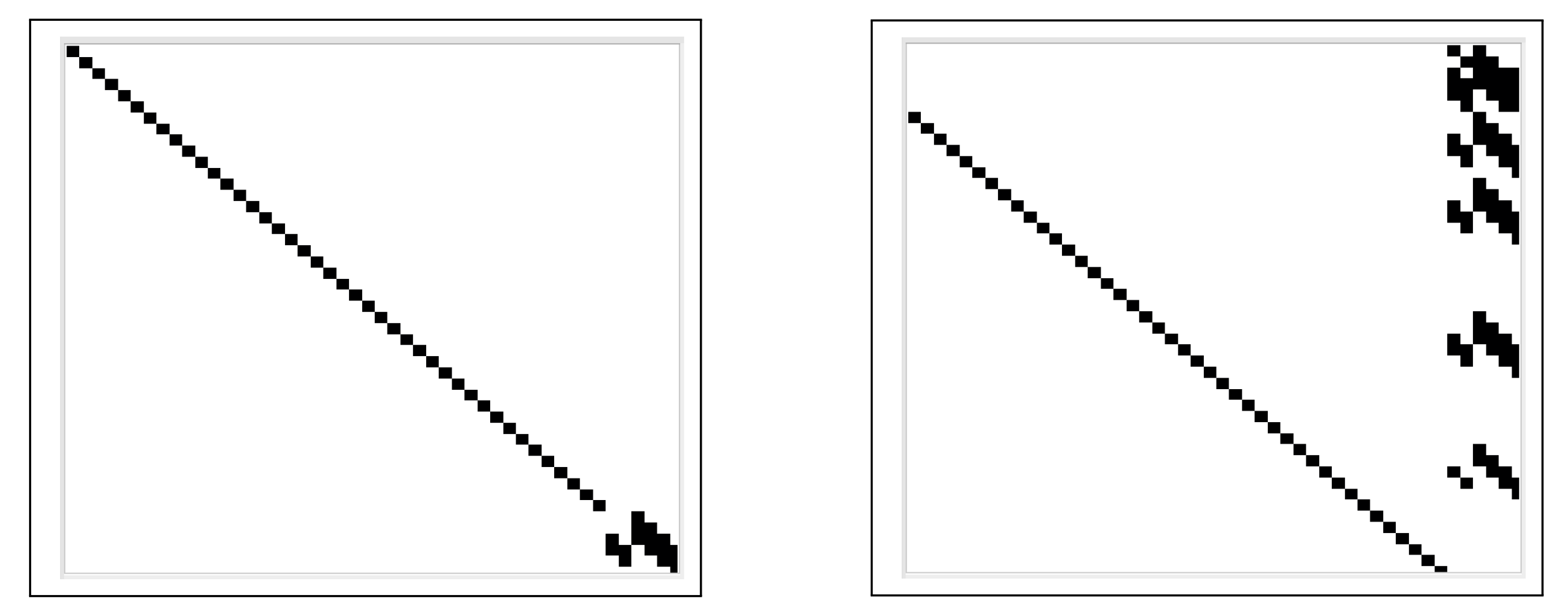
Remark 4.

The determinantal expressions derived for the offset to conics and quadrics show very good behavior when solving intersection queries through a generalized eigenvalue problem: they eliminate infinite eigenvalues and the pencil of matrices derived from these determinants is very sparse. The shape of the two matrices in the previous examples is reflected in Figure 5.

For the previous example, computing the huge polynomial $a_{\delta }(x\left(t\right),y\left(t\right),z\left(t\right))$ takes 0.562 s and determining its real roots 0.579 s, while the pencil of matrices is determined in 0.063 s and computing its generalized eigenvalues requires 0.07 s.

6. Conclusions

Starting from the implicit equations of conics and quadrics, we have introduced a new way to obtain the implicit equation of their corresponding offsets, highly efficient to solve geometric problems such as point positioning or for solving intersection problems. This new method consists of describing the offset directly as the discriminant of a characteristic equation. This new description, on the one hand, avoids the use of complex elimination techniques and, on the other, allows the use of typical tools for numerical matrix analysis, such as the generalized eigenvalues.