Optimal Control of Insect Populations

Abstract

We consider some optimal control problems for systems governed by linear parabolic PDEs with local controls that can move along the domain region $\Omega$ of the plane. We prove the existence of optimal paths and also deduce the first order necessary optimality conditions, using the Dubovitskii–Milyutin’s formalism, which leads to an iterative algorithm of the fixed-point kind. This problem may be considered as a model for the control of a mosquito population existing in a given region by using moving insecticide spreading devices. In this situation, an optimal control is any trajectory or path that must follow such spreading device in order to reduce the population as much as possible with a reasonable not too expensive strategy. We illustrate our results by presenting some numerical experiments.

1. Introduction

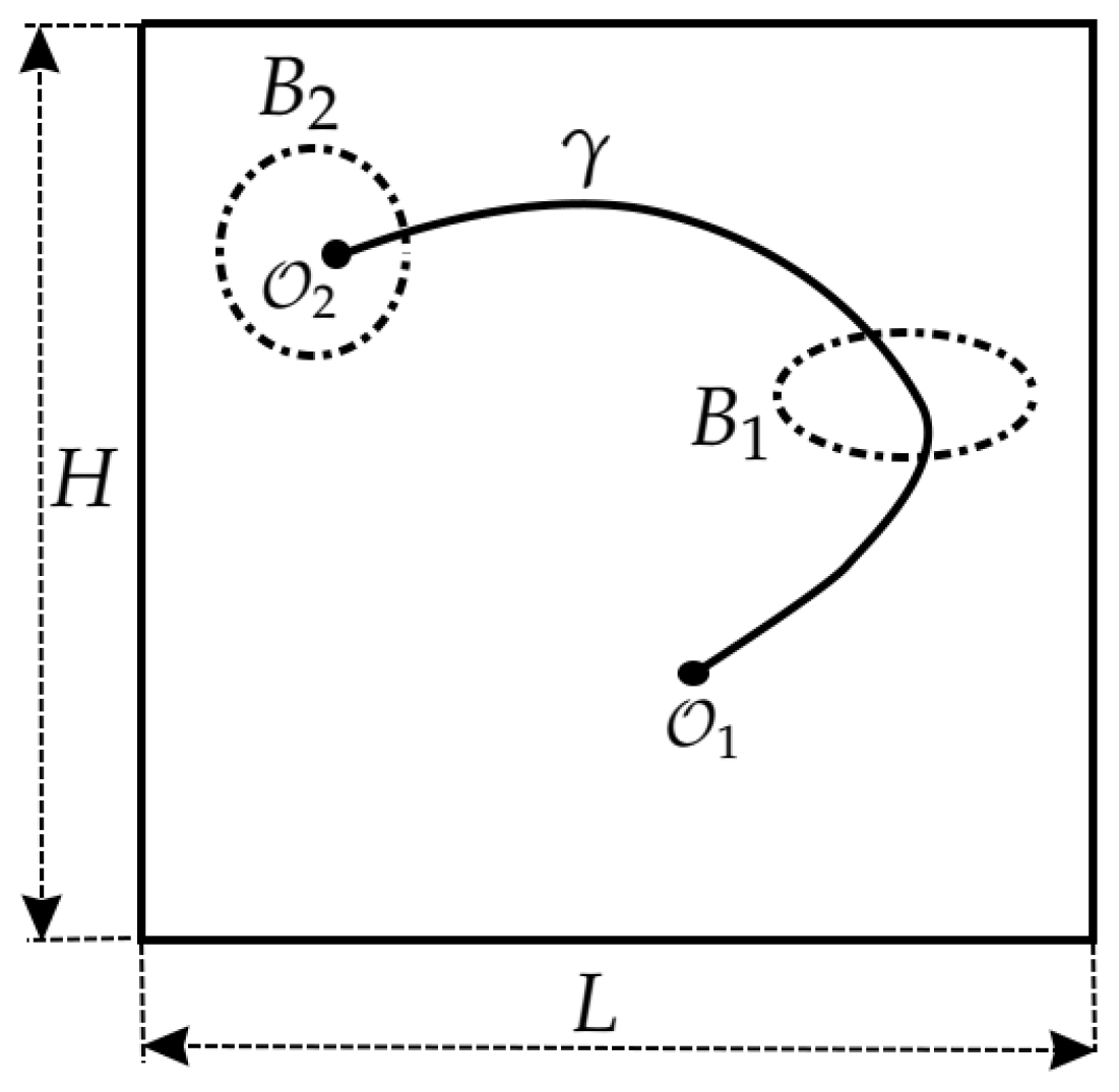
In this paper, we present and solve theoretically and numerically some optimal control problems concerning the extinction of mosquito populations by using moving devices whose main role is to spread insecticide. The controls are the trajectories or paths followed by the devices and the states are the resulting mosquito population densities. Thus, the unknowns in the considered problems are couples $(\gamma ,u)$, where $\gamma$ is a curve in the plane (see Figure 1), and u indicates how many mosquitoes there are and where they stay. The goal is to compute a trajectory leading to a minimal cost, measured in terms of operational costs and total population up to a final time.

The main simplifying assumptions for the model are the following:

Assumption 1.

Mosquitoes grow at a not necessarily constant known rate $a=a(x,t)$ and diffuses at a known constant rate α.

Assumption 2.

The insecticide immediately kills a fixed fraction of the population at a rate that decreases with the distance to the spreading source.

Assumption 3.

There are no obstacles for the admissible trajectories.

These assumptions can be relaxed in several ways.

For the problems considered in this paper, we prove the existence of an optimal solution, that is, a trajectory that leads to the best possible status of the system. We also characterize the optimal control–state pairs by appropriate first order optimality conditions. As usual, this is a coupled system that must be satisfied by any optimal control, its associated state, and an additional variable (the adjoint state) and must be viewed as a necessary condition for optimality.

In this paper, this characterization is obtained by using the so-called Dubovitskii–Milyutin techniques (see, for instance, Girsanov [1]). This relies on the following basic idea: on a local minimizer, the set of descent directions for the functional to minimize must be disjoint to the intersection of the cones of admissible directions determined by the restrictions. Accordingly, in view of Hahn-Banach’s Theorem, there exist elements in the associated dual cones, not all zero, whose sum vanishes. This algebraic condition is in fact the Euler–Lagrange equation for the problem in question. In order to be applied in our context, we must carry out the task of identifying all these (primal and dual) cones.

This formalism has been applied with success to several optimal control problems for PDEs, including the FitzHugh–Nagumo equation Brandao et al. [2]; solidification Boldrini et al. [3], the evolutionary Boussinesq model Boldrini et al. [4]; the heat equation Gayte et al. [5] and, also, some ecological systems that model the interaction of three species Coronel et al. [6].

We remark that part of the results presented here have their origin in ones in the Ph.D. thesis of Araujo [7].

This paper is organized as follows: Section 2 is devoted to describe the main achievements. The next two sections will be devoted to the rigorous proof of the optimality conditions; Section 3 contains some preparatory material and Section 4 deals with the main part of the proof. In Section 5, we deduce optimality conditions for a problem similar to the previous one, including in this case a restriction on the norm of the admissible trajectories. Once the optimality conditions are established, they can be used to devise numerical schemes to effectively compute suitable approximations of optimal trajectories; this will be explained in detail in Section 6. In Section 7, we present the results of numerical experiments performed with the numerical scheme described in the previous section. Finally, in Section 8, we present our conclusions and comment on further possibilities of investigation.

2. Main Achievements

Let $\Omega \subset {\mathbf{R}}^2$ be a non-empty bounded connected open set with boundary $\partial \Omega$ such that either $\partial \Omega$ is of class $C^2$ or $\Omega$ is a convex polygon and let $T>0$ be a given time. We want to find a curve ${\gamma }^{*}:[0,T]\mapsto {\mathbf{R}}^2$ such that

$$F\left({\gamma }^{*}\right)=\underset{\gamma \in \mathcal{V}}{min}F\left(\gamma \right),$$

(1)

where $\mathcal{V}:=\{\gamma \in H^1{(0,T)}^2:\gamma \left(0\right)=0\}$ is the space of admissible controls, and F is the following cost functional:

$${\displaystyle F\left(\gamma \right):={\mu }_0{\int }_0^T{|\gamma |}^{2}dt+{\mu }_1{\int }_0^T|\dot{\gamma }{|}^{2}dt+{\mu }_2\int {\int }_Q{|u|}^{2}dxdt,}$$

(2)

where $\dot{\gamma }$ is the time derivative of $\gamma$, and $u=u(x,t)$ is the associated state, that is, the unique solution to the problem

$$\left\{\begin{array}{cc}{\displaystyle u_t-\alpha \Delta u=a(x,t)u-bk(x-\gamma \left(t\right))u,}\hfill & \mathrm{in}Q:=\Omega \times (0,T),\hfill \\ {\displaystyle \frac{\partial u}{\partial \mathbf{n}}=0,}\hfill & \mathrm{on}S:=\partial \Omega \times (0,T),\hfill \\ u(x,0)=u_0,\hfill & \mathrm{in}\Omega .\hfill \end{array}\right.$$

(3)

Parameters ${\mu }_0\ge 0$, ${\mu }_1>0$, and ${\mu }_2>0$ are given constants. Concerning the interpretation of the cost functional (2), we observe that it can also be written in the form

$$F\left(\gamma \right):={\mu }_0{\parallel \gamma \parallel }_{L^2{(0,T)}^2}^2+{\mu }_1\parallel \dot{\gamma }{\parallel }_{L^2{(0,T)}^2}^2+{\mu }_2{\parallel u\parallel }_{L^2\left(Q\right)}^2.$$

The function $\gamma$ determines the trajectory of the device and $\dot{\gamma }$ is its corresponding velocity; moreover, the same path (geometric locus of the trajectory) can be traveled with different speeds leading to different operational costs. Since ${\parallel \gamma \parallel }_{L^2(0,T)}$ is a measure of the size of $\gamma$ and $\parallel \dot{\gamma }{\parallel }_{L^2(0,T)}$ is a measure of the velocity $\dot{\gamma }$, the quantity ${\mu }_0{\parallel \gamma \parallel }_{L^2(0,T)}^2+{\mu }_1{\parallel \dot{\gamma }\parallel }_{L^2(0,T)}^2$ can be regarded as a measure of the operational costs associated with the trajectory $\gamma$. Parameters ${\mu }_0$ and ${\mu }_1$ weight the relative importance being attributed to the size and the velocity of a trajectory in those operational costs. On the other hand, ${\parallel u\parallel }_{L^2\left(Q\right)}$ is a measure of the size of the mosquito population and ${\mu }_2$ is a constant parameter that weights the importance that is attributed to the decrease of such population.

It is expected that an improvement of the operational costs implies an increase of the effectiveness of the process and consequently leads to a reduction of the mosquito population, while a decrease of the operational costs leads to an increase of the mosquito population. Therefore, the minimization of F, once the parameters ${\mu }_0$, ${\mu }_1$, and ${\mu }_2$ are given, leads to a trajectory that balances the reduction of the mosquito population and the amount of operational costs. We remark that the values of ${\mu }_0$, ${\mu }_1$ and ${\mu }_2$ have a large influence on the shape of a possible optimal trajectory.

In short, $F\left(\gamma \right)$ is thus the sum of three terms, respectively related (but not coincident) to the length of the path travelled by the device, its speed along $(0,T)$ and the resulting population of insects. A maybe more realistic cost functional is indicated in Section 8.

In (3), $\alpha >0$, $b>0$, $a=a(x,t)$ is a non-negative function and $k:{\mathbf{R}}^2\mapsto \mathbf{R}$ is a positive $C^1$-function. The coefficient a is related to insect proliferation. It is standard in dynamics of population. In fact, in (3), the mosquito population u is assumed to have a space-time dependent Malthusian growth; this means that the population growth rate at each position and time is proportional to the number of individuals. The model admits a non-constant a to cope with the possibility of geographical places and times with different effects; for instance, more favorable growth rates occur in places with the presence of bodies of water or during rainy seasons.

As we mentioned in the Introduction, we assume that the insecticide immediately kills a fraction of the mosquito population present at a position x and time t, with a rate that is proportional to the insecticide concentration at that same position and time. At time t, the spreading device is at position $\gamma \left(t\right)$ and spreads a cloud of insecticide around it; the resulting insecticide concentration at any point x then depends on the position of x relative to $\gamma \left(t\right)$ (we expect that such concentration decays with the distance from the device). The spatial distribution of this concentration is then mathematically described as $k(x-\gamma \left(t\right))c_{max}$, where $c_{max}$ is the maximal spreading concentration capacity of the device, and k is a known $C^1$-function such that $0\le k\le 1$ and $k\left(\mathbf{0}\right)=1$. Then, the associated effective killing rate of the mosquito population is proportional to the product of insecticide concentration and the mosquito population. That is, $fk(x-\gamma \left(t\right))c_{max}u(x,t)$ for some proportionality factor f. By introducing $b=f{c}_{max}$, we get that the killing rate at position x and time t is $bk(x-\gamma (t\left)\right)u(x,t)$.

In our present analysis, it is not strictly needed but is natural to view k as an approximation of the Dirac distribution. For instance, it is meaningful to take

$$k\left(z\right):=k_0{e}^{-{|z|}^2/\sigma }$$

for some $k_0,\sigma >0$; this means that the device action in (3) at time t is maximal at $x=\gamma \left(t\right)$ and negligeable far from $\gamma \left(t\right)$. To this respect, see the choice of k in the numerical experiments in Section 7.

Of course, we can consider more elaborate models and include additional (nonlinear) terms in (3) related to competition; this is not done here just for simplicity of exposition.

Any solution $({\gamma }^{*},u^{*})$ to (1) provides an optimal trajectory and the associated population of mosquitoes. The existence of such a pair $({\gamma }^{*},u^{*})$ is established below, see Section 4.

As already mentioned, we also provide in this paper a characterization of optimal control–state pairs. It will be seen that, in the particular case of (1), the main consequence of the Dubovitskii–Milyutin method is the following: if ${\gamma }^{*}$ is an optimal control and $u^{*}$ is the associated state, there exists $p^{*}$ (the adjoint state), such that the following optimality conditions are satisfied:

$$\left\{\begin{array}{cc}{\displaystyle u_t^{*}-\alpha \Delta u^{*}=a(x,t)u^{*}-bk(x-{\gamma }^{*})u^{*},}\hfill & \hfill \mathrm{in}Q,\\ {\displaystyle \frac{\partial u^{*}}{\partial \mathbf{n}}=0,}\hfill & \hfill \mathrm{on}S,\\ {\displaystyle u^{*}(x,0)=u_0,}\hfill & \hfill \mathrm{in}\Omega ,\end{array}\right.$$

(4)

$$\left\{\begin{array}{cc}{\displaystyle -p_t^{*}-\alpha \Delta p^{*}=a(x,t)p^{*}-bk(x-{\gamma }^{*})p^{*}-2{\mu }_2{u}^{*},}\hfill & \hfill \mathrm{in}Q,\\ {\displaystyle \frac{\partial p^{*}}{\partial \mathbf{n}}=0,}\hfill & \hfill \mathrm{on}S,\\ {\displaystyle p^{*}(x,T)=0,}\hfill & \hfill \mathrm{in}\Omega \end{array}\right.$$

(5)

and

$$\left\{\begin{array}{cc}{\displaystyle -2{\mu }_1{\ddot{\gamma }}^{*}+2{\mu }_0{\gamma }^{*}-b{\int }_{\Omega }{p}^{*}{u}^{*}\nabla k(x-{\gamma }^{*})dx=0,}\hfill & \hfill \mathrm{in}(0,T),\\ {\displaystyle {\gamma }^{*}\left(0\right)=0,{\dot{\gamma }}^{*}\left(T\right)=0.}\hfill \end{array}\right.$$

(6)

3. Preliminaries

As usual, $\mathcal{D}(\Omega )$ will stand for the space of the functions in $C^{\infty }(\Omega )$ with compact support in $\Omega$ and $W^{r,p}(\Omega )$ and $H^m(\Omega )=W^{m,2}(\Omega )$ will stand for the usual Sobolev spaces; see Adams [8] for their definitions and properties. The gradient and Laplace operators will be respectively denoted by ∇ and $\Delta$.

The constants ${\mu }_0\ge 0$, ${\mu }_1>0$, ${\mu }_2>0$, $\alpha >0$ and $b>0$ and the functions k, $u_0$ and a are given, with

$$k\in C_b^1\left({\mathbf{R}}^2\right),0\le k\le 1,u_0\in H^1(\Omega )\mathrm{and}a\in L^{\infty }\left(Q\right).$$

In the sequel, C will denote a generic positive constant and the symbol $\langle ··\rangle$ will stand for several duality pairings.

Very frequently, the following spaces will be needed:

$$W_2^{2,1}\left(Q\right):=\{u\in L^2\left(Q\right):D^{\sigma }u\in L^2\left(Q\right)\forall 1\le |\sigma |\le 2,u_t\in L^2\left(Q\right)\}$$

and

$$W_{2,N}^{2,1}\left(Q\right):=\{u\in W_2^{2,1}\left(Q\right):\frac{\partial u}{\partial \mathbf{n}}=0\mathrm{on}S\}.$$

For the main results concerning these spaces, we refer, for instance, to [9]. Let us just recall one of them that is sometimes called the Lions–Peetre Embedding Theorem, see ([10], p. 13):

Lemma 1.

The embedding $W_2^{2,1}\left(Q\right)\hookrightarrow L^r\left(Q\right)$ is compact for all $1\le r<+\infty$.

For any Banach space B, we will denote by ${\parallel ·\parallel }_B$ the corresponding norm. Its topological dual space will be denoted by $B^{\prime }$. Recall that, if $K\subset B$ is a cone, the associated dual cone is the following:

$$K^{*}=\{f\in B^{\prime }:f\left(e\right)\ge 0\forall e\in K\}.$$

Let $A\subset B$ be given and let us assume that $e_0\in A$. It will be said that a nonzero linear form $f\in B^{\prime }$ is a support functional for A at $e_0$ if

$$f\left(e\right)\ge f\left(e_0\right)\forall e\in A.$$

Let Z be a Banach space and let $M:B\mapsto Z$ be a mapping. For any $e_0,e_1\in B$, we will denote by $M^{\prime }\left(e_0\right)e_1$ the Gateaux-derivative of M at $e_0$ in the direction $e_1$ whenever it exists. For obvious reasons, in the particular case $Z=\mathbf{R}$, this quantity will be written in the form $\langle M^{\prime }\left(e_0\right),e_1\rangle$.

The following result is known as Aubin–Lions’ Immersion Theorem. In fact, this version was given by Simon in [11], see p. 85, Corollary 4:

Lemma 2.

Let X, B, and Y be Banach spaces such that $X\hookrightarrow B\hookrightarrow Y$ with continuous embeddings, the first of them being compact and assume that $0<T<+\infty$. Then, the following embeddings are compact:

• ${\displaystyle L^q(0,T;X)\cap \{\varphi :{\varphi }_t\in L^1(0,T;Y)\}\hookrightarrow L^q(0,T;B)}$ for all $1\le q\le \infty$.
• ${\displaystyle L^{\infty }(0,T;X)\cap \{\varphi :{\varphi }_t\in L^r(0,T;Y)\}\hookrightarrow C^0([0,T];B)}$ for all $1<r\le \infty$.

The following result guarantees the existence and uniqueness of a state for each control $\gamma$ in the space of admissible controls $\mathcal{V}$:

Theorem 1.

For each $\gamma \in \mathcal{V}$, there exists a unique solution $u\in W_{2,N}^{2,1}\left(Q\right)$ of problem (3) satisfying the estimate

$${\parallel u\parallel }_{W_2^{2,1}\left(Q\right)}\le C{\parallel u_0\parallel }_{H^1(\Omega )}.$$

The constant C only depends on T, α, ${\parallel a\parallel }_{L^{\infty }\left(Q\right)}$, b, ${\parallel k\parallel }_{L^{\infty }\left({\mathbf{R}}^2\right)}$ and Ω.

For completeness, let us also recall an existence–uniqueness result for the adjoint system:

Theorem 2.

Let $\gamma \in \mathcal{V}$ and $u\in L^2\left(Q\right)$ be given. The linear system

$$\left\{\begin{array}{cc}{\displaystyle -p_t-\alpha \Delta p=a(x,t)p-bk(x-\gamma )p+2{\mu }_{2}u,}\hfill & \hfill \mathrm{in}Q,\\ {\displaystyle \frac{\partial p}{\partial \mathbf{n}}=0,}\hfill & \hfill \mathrm{on}S,\\ {\displaystyle p(x,T)=0,}\hfill & \hfill \mathrm{in}\Omega ,\end{array}\right.$$

(7)

possesses exactly one solution $p\in W_{2,N}^{2,1}\left(Q\right)$ such that

$${\parallel p\parallel }_{W_2^{2,1}\left(Q\right)}\le C{\parallel u_0\parallel }_{H^1(\Omega )},$$

with C as in Theorem 1.

We finish this section by recalling the Dubovitskii–Milyutin method. The presentation is similar to that in Boldrini et al. [3].

Let X be a Banach space and let $J:X\mapsto \mathbf{R}$ be a given function. Consider the extremal problem

$$J\left(e^{*}\right)=\underset{e\in \mathcal{Q}={\bigcap }_{\ell =1}^{n+1}{\mathcal{Q}}_{\ell }}{min}J\left(e\right)$$

(8)

where the ${\mathcal{Q}}_{\ell }$$(\ell =1,\cdots ,n+1)$ are by definition the restriction sets. It is assumed that

$$\mathrm{Int}{\mathcal{Q}}_i\ne Ø\forall 1\le i\le nand\mathrm{Int}{\mathcal{Q}}_{n+1}=Ø.$$

(9)

There are many situations where (9) holds In particular, the following holds:

• For any $1\le i\le n$, ${\mathcal{Q}}_i$ is an inequality restriction set of the form

  $${\mathcal{Q}}_i=\{e\in X:p_i\left(e\right)\le a_i\},$$

  where the $p_i:X\mapsto \mathbf{R}$ are continuous seminorms and the  $a_i>0$.
• ${\mathcal{Q}}_{n+1}$ is the equality restriction set

  $${\mathcal{Q}}_{n+1}=\{e\in X:M\left(e\right)=0\},$$

  where $M:X\mapsto Z$ is a differentiable mapping (Z is another Banach space).

The following theorem is a generalized version of the Dubovitskii–Milyutin principle and will be used in Section 4 and Section 5:

Theorem 3.

Let $e_0\in {\cap }_{\ell =1}^{n+1}{Q}_i$ be a local minimizer of problem (8) Let $D{C}_0$ be the decreasing cone of the cost functional J at $e_0$, let $F{C}_i$ be the feasible (or admissible) cone of ${\mathcal{Q}}_i$ at $e_0$ for $1\le i\le n$, and let $TC$ be the tangent cone to ${\mathcal{Q}}_{n+1}$ at $e_0$. Suppose that

• The cones $D{C}_0$ and $F{C}_i$$(1\le i\le n)$ are non-empty, open, and convex.
• The cone $TC$ is non-empty, closed, and convex.

Then

$$D{C}_0\cap \left(\bigcap _{i=1}^{n}F{C}_i\right)\cap TC=Ø.$$

Consequently, there exist $G_0\in {\left[D{C}_0\right]}^{*}$, $G_i\in {\left[F{C}_i\right]}^{*}$$(1\le i\le n)$ and $G_{n+1}\in {\left[TC\right]}^{*}$, not all zero, such that

$$G_0+\sum _{i=1}^n{G}_i+G_{n+1}=0.$$

In order to identify the decreasing, feasible, and tangent cones, we will use the following well known definitions and facts:

• Assume that $J:X\mapsto \mathbf{R}$ is Fréchet-differentiable. Then, for any $e\in X$, the decreasing cone of J at e is open and convex and is given by

  $$DC=\{h\in X:\langle J^{\prime }\left(e\right),h\rangle <0\},$$

  where $\langle ··\rangle$ stands for the usual duality product associated with X and $X^{\prime }$.
• Suppose that the set $\mathcal{Q}\subset X$ is convex, $\mathrm{Int}\mathcal{Q}\ne Ø$ and $e\in \mathcal{Q}$. Then, the feasible cone of $\mathcal{Q}$ at e is open and convex and is given by

  $$FC=\{\mu (e^{\prime }-e):e^{\prime }\in \mathrm{Int}\mathcal{Q},\mu >0\}.$$
• Finally, we have the celebrated Ljusternik Inverse Function Theorem; see, for instance, ([12], p. 167). The statement is the following: suppose that X and Y are Banach spaces, $M:X\mapsto Y$ is a mapping and the set

  $$\mathcal{Q}:=\{e\in X:M(e)=0\}$$

  is non-empty; in addition, suppose that $e_0\in \mathcal{Q}$, M is strictly differentiable at $e_0$ and $R\left(M^{\prime }\left(e_0\right)\right)=Y$; then, M maps a neighborhood of $e_0$ onto a neighborhood of 0 and the tangent cone to $\mathcal{Q}$ at $e_0$ is the closed subspace:

  $$TC=N\left(M^{\prime }\left(\xi \right)\right)=\{h\in X:M^{\prime }\left(e_0\right)h=0\}.$$

4. A First Optimal Control Problem

In this section, we will consider the optimal control problem (1)–(3). We will introduce an equivalent reformulation as an extremal problem of the kind (8). Then, we will prove that there exist optimal control–state pairs. Finally, we will use Theorem 3 to deduce appropriate (first order) necessary optimality conditions.

Our problem is the following:

$${\displaystyle \underset{(\gamma ,u)\in U_{ad}}{min}J(\gamma ,u),}$$

(10)

where J is given by (2) for any $(\gamma ,u)\in \mathcal{V}\times L^2\left(Q\right)$, and the set of admissible control–state pairs ${\mathcal{U}}_{ad}$ is defined by

$${\mathcal{U}}_{ad}:=\{(\gamma ,u)\in \mathcal{V}\times W_{2,N}^{2,1}\left(Q\right):M(\gamma ,u)=0\}.$$

(11)

Here,

$$M:\mathcal{V}\times W_{2,N}^{2,1}\left(Q\right)\mapsto L^2\left(Q\right)\times H^1(\Omega )$$

is the mapping defined by $M(\gamma ,u)=(\psi ,\phi )$, with

$$\left\{\begin{array}{c}\psi =M_1(\gamma ,u):=u_t-\alpha \Delta u-au+bk(x-\gamma )u\hfill \\ \phi =M_2(\gamma ,u):=u(·0)-u_0.\hfill \end{array}\right.$$

(12)

Theorem 4.

The extremal problem (10) possesses at least one solution.

Proof. 

Let us first check that ${\mathcal{U}}_{ad}$ is non-empty.

Let $\gamma \in \mathcal{V}$ be given. Then, from Theorem 1, there exists a unique solution $u\in W_{2,N}^{2,1}\left(Q\right)$ to (3) that, in particular, satisfies $M(\gamma ,u)=0$. Thus, we have $(\gamma ,u)\in {\mathcal{U}}_{ad}$.

Let us now see that ${\mathcal{U}}_{ad}$ is sequentially weakly closed in $\mathcal{V}\times L^2\left(Q\right)$. Thus, assume that $({\gamma }_n,u_n)\in {\mathcal{U}}_{ad}$ for all n and

$${\gamma }_n\to \gamma \mathrm{weakly}\mathrm{in}\mathcal{V}\mathrm{and}{u}_n\to u\mathrm{weakly}\mathrm{in}{L}^2\left(Q\right).$$

(13)

Then, ${\gamma }_n$ converges uniformly to $\gamma$ in $[0,T]$. Since $u_n$ is the unique solution to (3) with $\gamma$ replaced by ${\gamma }_n$, we necessarily have that u is the state associated with $\gamma$, that is, $(\gamma ,u)\in {\mathcal{U}}_{ad}$ and ${\mathcal{U}}_{ad}$ are certainly sequentially weakly closed.

Obviously, $J(\gamma ,u)$ is a well defined real number for any $(\gamma ,u)\in {\mathcal{U}}_{ad}$. Furthermore, $J:\mathcal{V}\times L^2\left(Q\right)\mapsto \mathbf{R}$ is continuous and (strictly) convex. Consequently, J is sequentially weakly lower semicontinuous in $\mathcal{V}\times L^2\left(Q\right)$.

Finally, J is coercive, i.e., it satisfies

$$J({\gamma }_n,u_n)\to +\infty \mathrm{as}{\parallel ({\gamma }_n,u_n)\parallel }_{\mathcal{V}\times L^2\left(Q\right)}\to +\infty .$$

Therefore, J attains its minimum in the weakly closed set ${\mathcal{U}}_{ad}$, and the result holds.    □

Remark 1.

Note that, although J is strictly convex, we cannot guarantee the uniqueness of solution to (10), since the admissible set ${\mathcal{U}}_{ad}$ is not necessarily convex. See, however, Remark 3 for a discussion on uniqueness.

In the next result, we specify the optimality conditions that must be satisfied by any solution to the extremal problem (10):

Theorem 5.

Let $({\gamma }^{*},u^{*})\in \mathcal{V}\times W_{2,N}^{2,1}\left(Q\right)$ be an optimal control–state pair for (10). Then, there exists $p^{*}\in W_{2,N}^{2,1}\left(Q\right)$ such that the triplet $({\gamma }^{*},u^{*},p^{*})$ satisfies (4)–(6).

We will provide a proof based on the Dubovitskii–Milyutin’s formalism, i.e., Theorem 3. Before, let us establish some technical results.

First of all, the functional $J:\mathcal{V}\times L^2\left(Q\right)\mapsto \mathbf{R}$ is obviously $C^{\infty }$ and the derivative of J at $(\gamma ,u)$ in the direction $(\beta ,v)$ is given by

$$\left\{\begin{array}{c}{\displaystyle \langle J^{\prime }(\gamma ,u),(\beta ,v)\rangle =2{\mu }_0{\int }_0^T\gamma ·\beta dt+2{\mu }_1{\int }_0^T\dot{\gamma }·\dot{\beta }dt+2{\mu }_2\int {\int }_{Q}uvdxdt}\hfill \\ {\displaystyle \forall (\gamma ,u),(\beta ,v)\in \mathcal{V}\times L^2\left(Q\right).}\hfill \end{array}\right.$$

(14)

Consequently, we have the following:

Lemma 3.

For each $(\gamma ,u)\in \mathcal{V}\times L^2\left(Q\right)$, the cone of decreasing directions of J at $(\gamma ,u)$ is

$$DC(\gamma ,u)=\{(\beta ,v)\in \mathcal{V}\times L^2\left(Q\right):\langle J^{\prime }(\gamma ,u),(\beta ,v)\rangle <0\}.$$

The associated dual cone is

$${\left[DC(\gamma ,u)\right]}^{*}=\{-\lambda J^{\prime }(\gamma ,u):\lambda \ge 0\}.$$

Lemma 4.

Let $(\gamma ,u)\in \mathcal{V}\times W_{2,N}^{2,1}\left(Q\right)$ be given.

(i)

Then, M is G-differentiable at $(\gamma ,u)$. The G-derivative of M at $(\gamma ,u)$ in the direction $(\beta ,v)$ is given by

$$M^{\prime }(\gamma ,u)(\beta ,v)=(M_1^{\prime }(\gamma ,u)(\beta ,v),M_2^{\prime }(\gamma ,u)(\beta ,v)),$$

where

$$\left\{\begin{array}{c}{M}_1^{\prime }(\gamma ,u)(\beta ,v):=v_t-\alpha \Delta v-av+bk(x-\gamma )v-b(\nabla k(x-\gamma )·\beta )u,\hfill \\ M_2^{\prime }(\gamma ,u)(\beta ,v):=v\left(0\right).\hfill \end{array}\right.$$

(15)

(ii)

The mapping M is $C^1$ in a neighborhood of $(\gamma ,u)$. Furthermore, $M^{\prime }(\gamma ,u)$ is surjective.

Proof. 

In order to prove (i), we use the definition of the Gâteaux-derivative. First, note that

$$\begin{array}{c}{\displaystyle \frac{1}{h}\left(M_1(\gamma +h\beta ,u+hv)-M_1(\gamma ,u)\right)-M_1^{\prime }(\gamma ,u)(\beta ,v)}\hfill \\ {\displaystyle =b\left[k(x-(\gamma +h\beta \left)\right)-k(x-\gamma )\right]v}\hfill \\ {\displaystyle +b\left(\frac{1}{h}\left[k(x-(\gamma +h\beta \left)\right)-k(x-\gamma )\right]-\nabla k(x-\gamma )·\beta \right)u,}\hfill \end{array}$$

while

$$\frac{1}{h}\left(M_2(\gamma +h\beta ,u+hv)-M_2(\gamma ,u)\right)-M_2^{\prime }(\gamma ,u)(\beta ,v)\equiv 0.$$

Therefore, in view of the assumptions on k, (15) and Lebesgue’s Theorem, it follows that

$$\frac{1}{h}\left(M(\gamma +h\beta ,u+hv)-M(\gamma ,u)\right)-M^{\prime }(\gamma ,u)(\beta ,v)\to 0\mathrm{as}h\to 0$$

strongly in $L^2\left(Q\right)\times H^1(\Omega )$, which proves (i).

We will now prove (ii). It is clear that, for any $(\gamma ,u)\in \mathcal{V}\times W_{2,N}^{2,1}\left(Q\right)$, $M^{\prime }(\gamma ,u)$ is a well defined continuous linear operator on $\mathcal{V}\times W_{2,N}^{2,1}\left(Q\right)$. Let $(\beta ,v)\in \mathcal{V}\times W_{2,N}^{2,1}\left(Q\right)$ be given and let us assume that $({\gamma }_n,u_n)\in \mathcal{V}\times W_{2,N}^{2,1}\left(Q\right)$ for all n and $({\gamma }_n,u_n)\to (\gamma ,u)$ strongly in $\mathcal{V}\times W_{2,N}^{2,1}\left(Q\right)$ as $n\to +\infty$. Then,

$$\begin{array}{c}{\displaystyle \parallel M_1^{\prime }({\gamma }_n,u_n)(\beta ,v)-M_1^{\prime }(\gamma ,u)(\beta ,v){\parallel }_{L^2\left(Q\right)}}\\ {\displaystyle \le b\parallel (k(·-{\gamma }_n)-k(·-\gamma )){v\parallel }_{L^2\left(Q\right)}+b\parallel (u_n\nabla k(·-{\gamma }_n)-u\nabla k(·-\gamma ))·\beta {)\parallel }_{L^2\left(Q\right)}.}\end{array}$$

In the last line, the first norm can be bounded as follows:

$$\parallel (k(·-{\gamma }_n)-k(·-\gamma )){v\parallel }_{L^2\left(Q\right)}\le \left(\underset{Q}{sup}|k(x-{\gamma }_n\left(t\right))-k(x-\gamma \left(t\right))|\right){\parallel v\parallel }_{L^2\left(Q\right)}.$$

Hence, from the hypotheses on k and the fact that ${\gamma }_n\to \gamma$ uniformly in $[0,T]$, we find that

$$\parallel (k(·-{\gamma }_n)-k(·-\gamma )){v\parallel }_{L^2\left(Q\right)}\le {ϵ}_n{\parallel v\parallel }_{L^2\left(Q\right)},\mathrm{with}{ϵ}_n\to 0.$$

(16)

On the other hand, we can deduce the following inequalities:

$$\begin{array}{c}{\displaystyle \parallel (u_n\nabla k(·-{\gamma }_n)-u\nabla k(·-\gamma ))·\beta {)\parallel }_{L^2\left(Q\right)}}\hfill \\ {\displaystyle \le \parallel (u_n-u)\nabla k(·-{\gamma }_n)·{\beta )\parallel }_{L^2\left(Q\right)}+\parallel u(\nabla k(·-{\gamma }_n)-\nabla k(·-\gamma ))·\beta {)\parallel }_{L^2\left(Q\right)}}\hfill \\ {\displaystyle \le \left(\underset{Q}{sup}|\nabla k(x-{\gamma }_n\left(t\right))·\beta \left(t\right)|\right){\parallel u_n-u\parallel }_{L^2\left(Q\right)}}\hfill \\ {\displaystyle +\left(\underset{Q}{sup}|(\nabla k(x-{\gamma }_n\left(t\right))-\nabla k(x-\gamma \left(t\right)))·\beta \left(t\right)|\right){\parallel u\parallel }_{L^2\left(Q\right)}}\hfill \\ {\displaystyle \le C\left[\parallel u_n{-u\parallel }_{L^2\left(Q\right)}+\left(\underset{Q}{sup}|\nabla k(x-{\gamma }_n\left(t\right))-\nabla k(x-\gamma \left(t\right))|\right){\parallel u\parallel }_{L^2\left(Q\right)}\right]{\parallel \beta \parallel }_{H^1{(0,T)}^2}.}\hfill \end{array}$$

Consequently, using again the hypotheses on k and the uniform convergence of ${\gamma }_n$, we can also write that

$$\parallel (u_n\nabla k(·-{\gamma }_n)-u\nabla k(·-\gamma ))·{\beta )\parallel }_{L^2\left(Q\right)}\le {ϵ}_n^{\prime }{\parallel \beta \parallel }_{H^1{(0,T)}^2},\mathrm{with}{ϵ}_n^{\prime }\to 0.$$

(17)

From (16) and (17), we find that

$$\parallel M_1^{\prime }({\gamma }_n,u_n)(\beta ,v)-M_1^{\prime }(\gamma ,u)(\beta ,v){\parallel }_{L^2\left(Q\right)}\le C({ϵ}_n+{ϵ}_n^{\prime }){\parallel (\beta ,v)\parallel }_{H^1{(0,T)}^2\times L^2\left(Q\right)}.$$

Since $M_2^{\prime }(\gamma ,u)$ is independent of $(\gamma ,u)$, we deduce that $(\gamma ,u)\mapsto M^{\prime }(\gamma ,u)$, regarded as a mapping from $\mathcal{V}\times W_{2,N}^{2,1}\left(Q\right)$ into $\mathcal{L}(\mathcal{V}\times W_{2,N}^{2,1}(Q);L^2(Q)\times H^1(\Omega ))$, is continuous.

Let us finally see that $M^{\prime }(\gamma ,u)$ is surjective.

Thus, let $(\phi ,\psi )$ be given in $L^2\left(Q\right)\times H^1(\Omega )$. We have to find $(\beta ,v)$ such that

$$M^{\prime }(\gamma ,u)(\beta ,v)=(\phi ,\psi ),(\beta ,v)\in \mathcal{V}\times W_{2,N}^{2,1}\left(Q\right).$$

(18)

However, this is easy: it suffices to first choose $\beta \in \mathcal{V}$ arbitrarily and then solve the linear problem:

$$\left\{\begin{array}{cc}{\displaystyle v_t-\alpha \Delta v=a(x,t)v-bk(x-\gamma )v+b(\nabla k(x-\gamma )·\beta )u+\phi }\hfill & \mathrm{in}Q\hfill \\ {\displaystyle \frac{\partial v}{\partial \mathbf{n}}=0}\hfill & \mathrm{on}S\hfill \\ v(x,0)=\psi \hfill & \mathrm{in}\Omega .\hfill \end{array}\right.$$

(19)

Obviously, the couple $(\beta ,v)$ satisfies (18).    □

From this lemma and Ljusternik’s Theorem, we obtain the following characterization of any tangent cone to ${\mathcal{U}}_{ad}$:

Lemma 5.

Let $(\gamma ,u)$ be given in ${\mathcal{U}}_{ad}$. Then, the tangent cone to ${\mathcal{U}}_{ad}$ at $(\gamma ,u)$ is the set

$$\begin{array}{c}{\displaystyle TC(\gamma ,u)=N\left(M^{\prime }(\gamma ,u)\right)}\hfill \\ {\displaystyle \phantom{TC(\gamma ,u)}:=\{(\beta ,v)\in \mathcal{V}\times W_{2,N}^{2,1}\left(Q\right):M^{\prime }(\gamma ,u)(\beta ,v)=0\}.}\hfill \end{array}$$

The associated dual cone is given by

$${\left[TC(\gamma ,u)\right]}^{*}=\{(\eta ,\zeta )\in {\mathcal{V}}^{\prime }\times W_{2,N}^{2,1}{\left(Q\right)}^{\prime }:\langle (\eta ,\zeta ),(\beta ,v)\rangle =0\forall (\beta ,v)\in TC(\gamma ,u)\}.$$

We can now present the proof of Theorem 5.

Proof of Theorem 5.

Let $({\gamma }^{*},u^{*})\in \mathcal{V}\times W_2^{2,1}\left(Q\right)$ be a solution to (10). The cone of decreasing directions of J at $({\gamma }^{*},u^{*})$ is

$$DC:=DC({\gamma }^{*},u^{*})=\{(\beta ,v)\in \mathcal{V}\times W_{2,N}^{2,1}(\Omega ):\langle J^{\prime }({\gamma }^{*},u^{*}),(\beta ,v)\rangle <0\}$$

and

$${\left[DC\right]}^{*}=\{-\lambda J^{\prime }({\gamma }^{*},u^{*}):\lambda \ge 0\}.$$

In addition, $({\gamma }^{*},u^{*})\in {\mathcal{U}}_{ad}$, the cone of tangent directions to ${\mathcal{U}}_{ad}$ at this point is

$$TC:=TC({\gamma }^{*},u^{*})=\{(\beta ,v)\in \mathcal{V}\times W_{2,N}^{2,1}\left(Q\right):M^{\prime }({\gamma }^{*},u^{*})(\beta ,v)=0\}$$

and

$${\left[TC\right]}^{*}=\{(\eta ,\zeta )\in {\mathcal{V}}^{\prime }\times W_{2,N}^{2,1}{\left(Q\right)}^{\prime }:\langle (\eta ,\zeta ),(\beta ,v)\rangle =0\forall (\beta ,v)\in TC\}.$$

From Theorem 3, we know that

$$DC\cap TC=Ø,$$

whence there must exist $G_0=-{\lambda }_0{J}^{\prime }({\gamma }^{*},u^{*})\in {\left[DC\right]}^{*}$ and also $G=(\eta ,\zeta )\in {\left[TC\right]}^{*}$, not simultaneously zero, such that

$$G_0+G=0.$$

Since ${\lambda }_0\ge 0$ and $G_0$ and G cannot be simultaneously zero, we necessarily have ${\lambda }_0>0$, and it can be assumed that ${\lambda }_0=1$.

Accordingly,

$$G=-G_0=J^{\prime }({\gamma }^{*},u^{*})$$

and

$${\displaystyle \langle (\eta ,\zeta ),(\beta ,v)\rangle =2\left({\displaystyle {\int }_0^T[{\mu }_0{\gamma }^{*}·\beta +{\mu }_1{\dot{\gamma }}^{*}·\dot{\beta }]dt+{\mu }_2\int {\int }_Q{u}^{*}vdxdt}\right)}$$

for all $(\beta ,v)\in \mathcal{V}\times W_{2,N}^{2,1}\left(Q\right)$. In particular, we see that

$${\displaystyle {\int }_0^T[{\mu }_0{\gamma }^{*}·\beta +{\mu }_1{\dot{\gamma }}^{*}·\dot{\beta }]dt+{\mu }_2\int {\int }_Q{u}^{*}vdxdt=0\forall (\beta ,v)\in TC.}$$

(20)

Now, let $\gamma \in \mathcal{V}$ be an arbitrary admissible control. Let w be the unique solution to the linear system:

$$\left\{\begin{array}{cc}{\displaystyle w_t-\alpha \Delta w=aw-bk(x-{\gamma }^{*})w+b(\nabla k(x-{\gamma }^{*})·\gamma )u^{*}}\hfill & \mathrm{in}Q\hfill \\ {\displaystyle \frac{\partial w}{\partial \mathbf{n}}=0}\hfill & \mathrm{on}S\hfill \\ {\displaystyle w(x,0)=0}\hfill & \mathrm{in}\Omega .\hfill \end{array}\right.$$

(21)

It follows from Lemma 5 that $(\gamma ,w)\in TC$, whence

$${\displaystyle {\int }_0^T\left[{\mu }_0{\gamma }^{*}·\gamma +{\mu }_1{\dot{\gamma }}^{*}·\dot{\gamma }\right]dt+{\mu }_2\int {\int }_Q{u}^{*}wdxdt=0.}$$

(22)

Let us introduce the adjoint system (5) and let us denote by $p^{*}$ its unique solution. By multiplying (21) by $-p^{*}$ and (5) by w, summing, integrating with respect to x and t and performing integrations by parts, we easily get that

$$\begin{array}{c}\hfill {\displaystyle b\int {\int }_Q{p}^{*}{u}^{*}(\nabla k(x-{\gamma }^{*})·\gamma )dxdt+{\displaystyle 2{\mu }_2\int {\int }_Q{u}^{*}wdxdt}=0.}\end{array}$$

(23)

Taking into account (22), we thus find that

$$\left\{\begin{array}{c}{\displaystyle {\int }_0^T\left[2{\mu }_0{\gamma }^{*}·\gamma +2{\mu }_1{\dot{\gamma }}^{*}·\dot{\gamma }\right]dt-b\int {\int }_Q{p}^{*}{u}^{*}\nabla k(x-{\gamma }^{*})·\gamma dxdt=0}\hfill \\ {\displaystyle \forall \gamma \in \mathcal{V};{\gamma }^{*}\in \mathcal{V}.}\hfill \end{array}\right.$$

(24)

However, this is just the weak formulation of the boundary problem (6). Indeed, standard arguments show that ${\gamma }^{*}$ solves (24) if and only if ${\gamma }^{*}\in H^1{(0,T)}^2$, the second-order integro-differential equation

$${\displaystyle -2{\mu }_1{\ddot{\gamma }}^{*}+2{\mu }_0{\gamma }^{*}-b{\int }_{\Omega }{p}^{*}(x,t)u^{*}(x,t)\nabla k(x-{\gamma }^{*}\left(t\right))dx=0}$$

holds in the distributional sense in $(0,T)$, ${\gamma }^{*}\left(0\right)=0$ and ${\dot{\gamma }}^{*}\left(T\right)=0$. Thus, the triplet $({\gamma }^{*},u^{*},p^{*})$ satisfies (4)–(6).

This ends the proof.    □

Remark 2.

There are other ways to prove Theorem 5. For instance, it is possible to apply an argument relying on Lagrange multipliers, starting from the Lagrangian

$$L(\gamma ,u,p):=J(\gamma ,u)+\langle p,M(\gamma ,u)\rangle .$$

That $({\gamma }^{*},u^{*})$ is an optimal control–state pair, and $p^{*}$ is an associated adjoint state (resp. that $({\gamma }^{*},u^{*},p^{*})$ satisfies the optimality conditions (4)–(6)) is formally equivalent to say that the triplet $({\gamma }^{*},u^{*},p^{*})$ is a saddle point (resp. a stationary point) of L.

Remark 3.

As already said, in general, there is no reason to expect uniqueness. However, in view of Theorem 5, it is reasonable to believe that, under appropriate assumptions on b and k, the solution is unique. Indeed, taking into account that $k^{\prime }$ is uniformly bounded in ${\mathbf{R}}^2$, if b is sufficiently small, $({\gamma }^i,u^i)$ is an optimal pair for $i=1,2$ and one sets $\gamma :={\gamma }^1-{\gamma }^2$, $u:=u^1-u^2$, the following is not difficult to prove:

• The $u^i$ are uniformly bounded (for instance) in $L^2\left(Q\right)$ by a constant of the form $e^{C(1+b)}$.
• u and p are bounded in $L^2\left(Q\right)$ by a constant of the form $b{e}^{C(1+b)}{\parallel \gamma \parallel }_{L^{\infty }}$.
• γ is bounded in $L^{\infty }(0,T)$ by a constant of the form $b{e}^{C(1+b)}{\parallel \gamma \parallel }_{L^{\infty }}$.

In these estimates, C depends on ${\parallel k\parallel }_{W^{1,\infty }\left({\mathbf{R}}^2\right)}$ and the other data of the problem but is independent of b. Consequently, if b is small enough, the solution to the optimal control problem is unique.

5. A Second Optimal Control Problem

This section deals with a more realistic second optimal control problem. Specifically, we will analyze the constrained problem

$$F\left({\gamma }^{*}\right)=\underset{\gamma \in \mathcal{B}}{min}F\left(\gamma \right),$$

(25)

where

$$\mathcal{B}:=\{\gamma \in H^1{(0,T)}^2:\gamma \left(0\right)=0,\parallel \gamma {\parallel }_{H^1{(0,T)}^2}\le R_0\}$$

(26)

and F is given by (2). Here, $R_0>0$ is a prescribed constant. We can interpret the constraint $\gamma \in \mathcal{B}$ as a limitation on the positions and the speed of the device; roughly speaking, a solution to (25) furnishes a strategy that leads to a minimal insect population (in the $L^2$ sense) with few resources.

For this problem, we will also prove the existence of optimal controls, and we will also find the optimality conditions furnished by the Dubovitskii–Milyutin formalism.

Thus, let ${\gamma }^{*}$ be an optimal control for this new problem, let $u^{*}$ and $p^{*}$ be the associated state and adjoint state and let us introduce the notation

$$m(\gamma ,\beta ):={\int }_0^T\left(2{\mu }_0\gamma ·\beta +2{\mu }_1\dot{\gamma }·\dot{\beta }\right)dt.$$

(27)

Then, it will be shown that the associated optimality conditions of first order are (4), (5) and

$$\left\{\begin{array}{c}{\displaystyle m({\gamma }^{*},\gamma -{\gamma }^{*})-b\int {\int }_Q{u}^{*}{p}^{*}\nabla k(x-{\gamma }^{*})(\gamma -{\gamma }^{*})dxdt\ge 0}\hfill \\ {\displaystyle \forall \gamma \in \mathcal{B};{\gamma }^{*}\in \mathcal{B}.}\hfill \end{array}\right.$$

(28)

The problem can be rewritten in the form

$${\displaystyle \underset{(\gamma ,u)\in {\mathcal{Z}}_{ad}}{min}J(\gamma ,u),}$$

(29)

where J is given by (2) and the set of admissible pairs ${\mathcal{Z}}_{ad}$ is

$${\mathcal{Z}}_{ad}:=\{(\gamma ,u)\in \mathcal{V}\times W_{2,N}^{2,1}\left(Q\right):M(\gamma ,u)={0,\parallel \gamma \parallel }_{H^1{(0,T)}^2}\le R_0\}.$$

(30)

Recall that $M=(M_1,M_2)$ is given by (12).

One has:

Theorem 6.

The extremal problem (29) possesses at least one solution.

The proof is similar to the proof of Theorem 4. Indeed, it is easy to check that ${\mathcal{Z}}_{ad}$ is a non-empty weakly closed subset of $\mathcal{V}\times L^2\left(Q\right)$. Since $J:\mathcal{V}\times L^2\left(Q\right)\mapsto \mathbf{R}$ is continuous, (strictly) convex and coercive, it also attains its minimum in ${\mathcal{Z}}_{ad}$, and this proves that (29) is solvable.

Theorem 7.

Let $({\gamma }^{*},u^{*})\in \mathcal{V}\times W_2^{2,1}\left(Q\right)$ be an optimal control–state pair for (29). Then, there exists $p^{*}\in W_2^{2,1}\left(Q\right)$ such that the triplet $({\gamma }^{*},u^{*},p^{*})$ satisfies (4), (5) and (28), where the bilinear form $m(··)$ is given by (27).

Proof. 

We will argue as in the proof of Theorem 5.

First, notice that ${\mathcal{Z}}_{ad}$ can be written in the form

$${\mathcal{Z}}_{ad}={\mathcal{U}}_{ad}\cap (\mathcal{B}\times L^2\left(Q\right))$$

Let $({\gamma }^{*},u^{*})\in \mathcal{V}\times W_2^{2,1}\left(Q\right)$ be a solution to (29). Then, the feasible cone of $\mathcal{B}\times L^2\left(Q\right)$ at $({\gamma }^{*},u^{*})$ is the set

$$FC:=FC({\gamma }^{*},u^{*})=\{(\mu (\gamma -{\gamma }^{*}),v):\gamma \in \mathrm{Int}\mathcal{B},\mu >0,v\in L^2\left(Q\right)\}$$

and

$${\left[FC\right]}^{*}=\{(h,0):h\mathrm{is}\mathrm{a}\mathrm{support}\mathrm{functional}\mathrm{of}\mathcal{B}\mathrm{at}{\gamma }^{*}\}.$$

Recall that the latter means that $h\in {\mathcal{V}}^{\prime }$ and

$$\langle h,\gamma \rangle \ge \langle h,{\gamma }^{*}\rangle \forall \gamma \in \mathcal{B}.$$

(31)

From Theorem 3, we now have

$$DC\cap TC\cap FC=Ø,$$

whence there exist $G_0=-{\lambda }_0{J}^{\prime }({\gamma }^{*},u^{*})\in {\left[DC\right]}^{*}$, $G=(\eta ,\zeta )\in {\left[TC\right]}^{*}$ and $H=(h,0)\in {\left[FC\right]}^{*}$, not simultaneously zero, such that

$$G_0+G+H=0.$$

As before, we necessarily have ${\lambda }_0>0$. Indeed, if ${\lambda }_0=0$, then

$$\langle (\eta ,\zeta ),(\gamma ,w)\rangle +\mu \langle h,\gamma \rangle =0\forall (\beta ,v)\in \mathcal{V}\times W_{2,N}^{2,1}\left(Q\right).$$

However, for any $\gamma \in \mathcal{V}$, we can always construct w in $W_{2,N}^{2,1}\left(Q\right)$ such that $(\gamma ,w)\in TC$. Hence, we would have $\langle (\eta ,\zeta ),(\gamma ,w)\rangle =0$ and $\mu \langle h,\gamma \rangle =0$ for all $\gamma \in \mathcal{V}$, which is impossible.

We can thus assume that ${\lambda }_0=1$ and

$$G+H=-G_0=J^{\prime }({\gamma }^{*},u^{*}).$$

In particular, we get:

$${\displaystyle {\int }_0^T[{\mu }_0{\gamma }^{*}·\beta +{\mu }_1{\dot{\gamma }}^{*}·\dot{\beta }]dt+{\mu }_2\int {\int }_Q{u}^{*}vdxdt=\langle h,\beta \rangle \forall (\beta ,v)\in TC.}$$

(32)

Let us consider again the adjoint system (5) and let us denote by $p^{*}$ its unique solution. Let $\gamma \in \mathcal{B}$ be an arbitrary admissible control and let w be the unique solution to (21). Since $(\gamma ,w)\in TC$ and we still have (23), we get:

$${\displaystyle {\displaystyle {\int }_0^T\left[2{\mu }_0{\gamma }^{*}·\gamma +2{\mu }_1{\dot{\gamma }}^{*}·\dot{\gamma }\right]dt}-b\int {\int }_Q{p}^{*}{u}^{*}\nabla k(x-{\gamma }^{*})·\gamma dxdt=\langle h,\gamma \rangle .}$$

(33)

Taking into account that $\gamma$ is arbitrary in $\mathcal{B}$ and (31) holds, we deduce that (28) is satisfied, and the result is proved.    □

6. A Numerical Scheme

In this section, we present a numerical scheme to find an approximate solution to (1)–(3). To this purpose, we will use the optimality conditions (4)–(6).

Obviously, we will have to approximate the equations in time and space. With respect to the time variable, we will incorporate finite differences taking into account the following:

• Since the equation (4) is parabolic, in order to guarantee unconditional stability, we discretize in time by using a backward Euler method. For the same reason, we discretize M in time in by using a forward Euler method.
• Since (6) is a second order two-point boundary value problem, we approximate there the time derivatives with a standard (centered) finite difference scheme.

Let N be a positive (large) integer and let us consider a partition ${\Lambda }_N=\{0=t_0,t_1,\dots ,t_N=T\}$ of the time interval $[0,T]$ in N subintervals. For simplicity, we assume that this partition is uniform, with time step $\Delta t:=T/N$.

On the other hand, the approximation in space will be performed via a finite element method. Thus, let ${\mathcal{T}}_h$ be a triangular mesh of a polynomial approximation ${\Omega }_h$ of $\Omega$ and let us denote by $V_h$ a suitable finite element space associated with ${\mathcal{T}}_h$. For instance, $V_h$ can be the usual $P_1$-Lagrange space, formed by the continuous piecewise linear functions on ${\Omega }_h$.

Then, given an approximation $u_h(·0)\in V_h$ of $u_0$, we must compute functions $u_h^N\left(t_i\right)$ and $p_h^N\left(t_i\right)$ and vectors ${\gamma }_h^N(t_i)=({\gamma }_{h,1}^N(t_i),{\gamma }_{h,2}^N(t_i))$ such that:

$$\left\{\begin{array}{c}{\displaystyle {\int }_{\Omega }\frac{u_h^N\left(t_i\right)-u_h^N\left(t_{i-1}\right)}{\Delta t}vdx+{\int }_{\Omega }\alpha \nabla u_h^N\left(t_i\right)·\nabla vdx}\hfill \\ {\displaystyle ={\int }_{\Omega }a(x,t_i)u_h^N\left(t_i\right)vdx-{\int }_{\Omega }bk(x-{\gamma }_h^N\left(t_i\right))u_h^N\left(t_i\right)vdx\forall v\in V_h}\hfill \\ u_h^N\left(t_0\right)=u_h(x,0),\hfill \end{array}\right.$$

(34)

$$\left\{\begin{array}{c}{\displaystyle {\int }_{\Omega }-\frac{p_h^N\left(t_i\right)-p_h^N\left(t_{i-1}\right)}{\Delta t}qdx+{\int }_{\Omega }\alpha \nabla p_h^N\left(t_{i-1}\right)·\nabla qdx}\hfill \\ {\displaystyle ={\int }_{\Omega }a(x,t)p_h^N\left(t_{i-1}\right)qdx-{\int }_{\Omega }bk(x-{\gamma }_h^N\left(t_{i-1}\right))p_h^N\left(t_{i-1}\right)qdx}\hfill \\ {\displaystyle -{\int }_{\Omega }2{\mu }_2{u}_h^N\left(t_{i-1}\right)qdx\forall q\in V_h}\hfill \\ p_h^N\left(t_N\right)=0,\hfill \end{array}\right.$$

(35)

$$\left\{\begin{array}{c}{\displaystyle -2{\mu }_1\frac{{\gamma }_h^N\left(t_{k-1}\right)-2{\gamma }_h^N\left(t_k\right)+{\gamma }_h^N\left(t_{k+1}\right)}{{(\Delta t)}^2}+2{\mu }_0{\gamma }_h^N\left(t_k\right)}\hfill \\ {\displaystyle -b{\int }_{\Omega }{p}_h^N\left(t_k\right)u_h^N\left(t_k\right)·\nabla k(x-{\gamma }_h^N\left(t_k\right))dx=0}\hfill \\ \mathrm{for}k=2,\dots ,N-1\hfill \\ {\displaystyle {\gamma }_h^N\left(t_0\right)=0,D_h{\gamma }_h^N\left(t_N\right)=0.}\hfill \end{array}\right.$$

(36)

In the last line of (36), $D_h$ denotes a suitable discrete operator associated with the time derivative. In our code, to preserve second order approximation in time, we took $D_h{\gamma }_h^N\left(t_N\right):=[{\gamma }_h^N\left(t_{N-1}\right)-{\gamma }_h^N\left(t_{N+1}\right)]/2\Delta t$, where $t_{N+1}=t_N+\Delta t$ is an additional time-mesh point. This implies that ${\gamma }_h^N\left(t_{N-1}\right)={\gamma }_h^N\left(t_{N+1}\right)$ and, thus, the required Neumann boundary condition can be imposed just using a reduced form of the finite difference operator at $t_N$, that is, ${\displaystyle [{\gamma }_h^N\left(t_{N-1}\right)-2{\gamma }_h^N\left(t_N\right)+{\gamma }_h^N\left(t_{N+1}\right)]{(\Delta t)}^2=[2{\gamma }_h^N\left(t_{N-1}\right)-2{\gamma }_h^N\left(t_N\right)]/{(\Delta t)}^2}$.

6.1. An Iterative Algorithm for Fixed N and ${\mathcal{T}}_h$

The previous finite dimensional system is nonlinear and, consequently, cannot be solved exactly. Accordingly, an iterative algorithm has been devised to obtain a solution. It is the following:

Base step:

Choose tolerances ${ϵ}_{\mathrm{outer}}>0$ and ${ϵ}_{\mathrm{inner}}>0$; by starting with ${\gamma }_{h,0}^N\equiv 0$, proceed recursively for $n=1,2,\dots$ in an outer iteration scheme as follows:

First step: Find $u_{h,n}^N$.

Since ${\gamma }_{h,n-1}^N\left(t_i\right)$ is known, advance in time to find $u_{h,n}^N\left(t_i\right)$, for $i=1,\dots ,N$, by successively solving the linear problems

$$\left\{\begin{array}{c}{\displaystyle {\int }_{\Omega }\frac{u_{h,n}^N\left(t_i\right)-u_{h,n}^N\left(t_{i-1}\right)}{\Delta t}vdx+{\int }_{\Omega }\alpha \nabla u_{h,n}^N\left(t_i\right)·\nabla vdx}\hfill \\ {\displaystyle ={\int }_{\Omega }a(x,t_i)u_{h,n}^N\left(t_i\right)vdx-{\int }_{\Omega }bk(x-{\gamma }_{h,n-1}^N\left(t_i\right))u_{h,n}^N\left(t_i\right)vdx\forall v\in V_h}\hfill \\ {\displaystyle u_{h,n}^N\left(t_0\right)=u_h\left(t_0\right).}\hfill \end{array}\right.$$

(37)

Second step: Find $p_{h,n}^N$.

Since ${\gamma }_{h,n-1}^N\left(t_i\right)$ and $u_{h,n}^N$ are known, proceed backwards in time to find $p_{h,n}^N\left(t_i\right)$, for $i=N-1,\dots ,0$, by solving the problems

$$\left\{\begin{array}{c}{\displaystyle {\int }_{\Omega }-\frac{p_{h,n}^N\left(t_i\right)-p_{h,n}^N\left(t_{i-1}\right)}{\Delta t}qdx+{\int }_{\Omega }\alpha \nabla p_{h,n}^N\left(t_{i-1}\right)·\nabla qdx}\hfill \\ {\displaystyle ={\int }_{\Omega }a(x,t)p_{h,n}^N\left(t_{i-1}\right)qdx-{\int }_{\Omega }bk(x-{\gamma }_{h,n-1}^N\left(t_{i-1}\right))p_{h,n}^N\left(t_{i-1}\right)qdx}\hfill \\ {\displaystyle -{\int }_{\Omega }2{\mu }_2{u}_{h,n}^N\left(t_{i-1}\right)qdx\forall q\in V_h}\hfill \\ p_{h,n}^N\left(t_N\right)=0.\hfill \end{array}\right.$$

(38)

Third step: Find ${\gamma }_{h,n}^N$.

This is done by applying an inner iteration scheme. Thus, by starting with ${\tilde{\gamma }}_0={\gamma }_{h,n-1}^N$, find recursively ${\{{\tilde{\gamma }}_m\}}_{m=1}^{\infty }$ by repeating the following for $m=1,2,\dots$:

$$\left\{\begin{array}{c}{\displaystyle -2{\mu }_1\frac{{\tilde{\gamma }}_m\left(t_{k-1}\right)-2{\tilde{\gamma }}_m\left(t_k\right)+{\tilde{\gamma }}_m\left(t_{k+1}\right)}{{(\Delta t)}^2}+2{\mu }_0{\tilde{\gamma }}_m\left(t_k\right)}\hfill \\ {\displaystyle -b{\int }_{\Omega }{p}_h^N\left(t_k\right)u_h^N\left(t_k\right)·\nabla k(x-{\tilde{\gamma }}_{m-1}\left(t_k\right))dx=0}\hfill \\ \mathrm{for}k=2,\dots ,N-1\hfill \\ {\displaystyle {\tilde{\gamma }}_m\left(t_0\right)=0,D_h{\tilde{\gamma }}_m\left(t_N\right)=0,}\hfill \end{array}\right.$$

(39)

with a meaning similar to above for $D_h{\tilde{\gamma }}_m\left(t_N\right)=0$. This is a finite linear system for ${\tilde{\gamma }}_m={[{\tilde{\gamma }}_m\left(t_1\right),\dots ,{\tilde{\gamma }}_m\left(t_N\right)]}^{\prime }$ where the coefficient matrix is independent of m and can thus be inverted only once, at the beginning of the process.

The relative stopping criterion for the iteration process is

$$max\left\{\frac{\parallel {\tilde{\gamma }}_m-{\tilde{\gamma }}_{m-1}\parallel }{\parallel {\tilde{\gamma }}_m\parallel },\frac{\parallel {\tilde{\gamma }}_m-{\tilde{\gamma }}_{m-1}\parallel }{\parallel {\tilde{\gamma }}_{m-1}\parallel }\right\}\le {ϵ}_{\mathrm{inner}}.$$

where $\parallel ·\parallel$ denotes the usual discrete $L^2$-norm. When this stopping criterion is satisfied, take ${\gamma }_{h,n}^N={\tilde{\gamma }}_n$ and proceed to the next step.

Fourth step: Compare ${\gamma }_{h,n}^N$ and ${\gamma }_{h,n-1}^N$.

When the overall relative stopping criterion

$$max\left\{\frac{\parallel u_{h,n}^N-u_{h,n-1}^N\parallel }{\parallel u_{h,n}^N\parallel },\frac{\parallel p_{h,n}^N-p_{h,n-1}^N\parallel }{\parallel p_{h,n}^N\parallel },\frac{\parallel {\gamma }_{h,n}^N-{\gamma }_{h,n-1}^N\parallel }{min\left(\parallel {\gamma }_{h,n}^N\parallel ,\parallel {\gamma }_{h,n-1}^N\parallel \right)}\right\}\le {ϵ}_{\mathrm{outer}}$$

is satisfied, stop the iterative process and take

$$u_h^N=u_{h,n}^N,p_h^N=p_{h,n}^N\mathrm{and}{\gamma }_h^N={\gamma }_{h,n}^N$$

as the computed approximated solutions. Otherwise, increase n by one and go back to the First step.

Acceleration of Algorithm

To accelerate the process, ${ϵ}_{inner}$ can be taken larger than ${ϵ}_{outer}$. In addition, to get a better resolution, in the final iterative scheme, we have allowed for a decrease of the time-step by increasing the number of time intervals N.

The resulting iterates are as follows:

Base step:

Give tolerances ${ϵ}_{\gamma }>0$, ${ϵ}_{\mathrm{outer}}>0$, ${ϵ}_{\mathrm{inner}}>0$ and an initial number of discrete time intervals $N_0\ge 1$.

First step:

Take $N=N_0$ and apply the previous iterative algorithm, to obtain $u_h^N$, $p_h^N$ and ${\gamma }_h^N$. Define ${\gamma }_{\mathrm{before}}={\gamma }_h^{N_0}$.

Second step:

Double the value of N and apply the previous algorithm to obtain new $u_h^N$, $p_h^N$ and ${\gamma }_h^N$.

Third step:

Compare ${\gamma }_h^N$ and ${\gamma }_{\mathrm{before}}$. If the convergence criterion

$$\frac{\parallel {\gamma }_h^N-{\gamma }_{\mathrm{before}}\parallel }{\parallel {\gamma }_h^N\parallel }\le {ϵ}_{\gamma }$$

is satisfied, stop the iterates and take as approximated solutions

$$u^{*}=u_{h,n}^N,p^{*}=p_{h,n}^N\mathrm{and}{\gamma }^{*}={\gamma }_{h,n}^N.$$

Otherwise, go back to the Second step and repeat the process.

7. Numerical Experiments

In order to illustrate the behavior of the previous algorithm, let us present the results of some experiments with $\Omega =[-2.5,2.5]\times [-2.5,2.5]$.

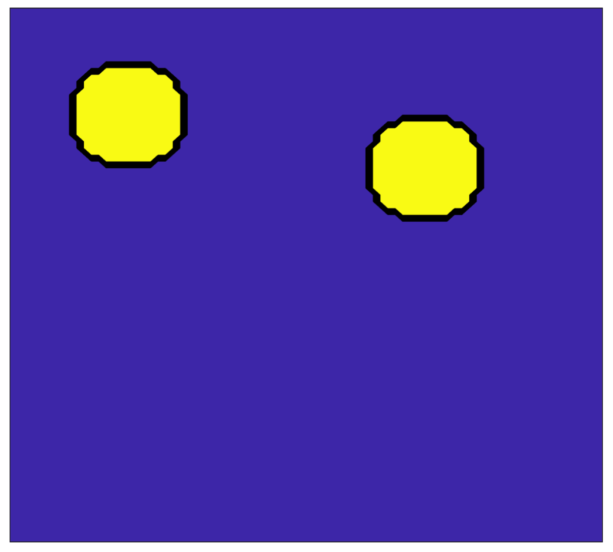
Let us denote by ${\mathbf{1}}_{\omega }$ the indicator function of $\omega$ for any $\omega \subset \Omega$; we consider an initial mosquito population given by

$$u_0\left(x\right)\equiv 10.0\times {\mathbf{1}}_{B_1}(x,y)+10.0\times {\mathbf{1}}_{B_2}(x,y),$$

where $B_1$ and $B_2$ are, respectively, the circle of center $(-1.5,1.5)$ and radius $0.5$ and the circle of center $(1.0,1.0)$ and radius $0.5$. This means that the mosquito population is initially concentrated in two disjoint circles with the same radius and the same amount of population, see Figure 2.

We also consider the following values for the parameters and functions in (3):

$$\alpha =1.0,b=10.0,k(x,y)\equiv exp[-(x^2+y^2)/{\left(0.5\right)}^2].$$

For the stopping criteria, we have taken

$${ϵ}_{\mathrm{outer}}=0.05\mathrm{and}{ϵ}_{\mathrm{inner}}=0.2.$$

The computations have been performed by using the software FreeFem++, [13] and all figures were made with Octave [14].

7.1. Convergence Behavior

In this section, we test the convergence of the algorithm described in Section 6.1. We take $a(x,t)\equiv 1.0$ in (3) and ${\mu }_0={\mu }_1={\mu }_2=1$. The numerical solution of the optimality system (4)–(6) is computed for several values of the final time T and the number of subintervals N:

$$\begin{array}{ccc}\hfill T& =& 2,4,6;\hfill \\ \hfill N& =& 50,100,200.\hfill \end{array}$$

Moreover, we consider three different regular meshes ${\mathcal{T}}_{h_k},k=1,2,3$, with $m\times m$ lateral nodes.

Table 1. Details of the meshes.

Number of Lateral	Mesh Nodes $\mathit{m}\times \mathit{m}$	Number of Size ${\mathit{h}}_{\mathit{k}}$	Number of Vertices ${\mathit{n}}_{\mathit{v}}$	Triangles ${\mathit{n}}_{\mathit{T}}$
Mesh 1	$20\times 20$	0.3536	441	800
Mesh 2	$40\times 40$	0.1768	1681	3200
Mesh 3	$80\times 80$	0.0884	6561	12,800

shows the size $h_k$, the number of vertices $n_v$, and the number of triangles $n_T$ for each mesh.

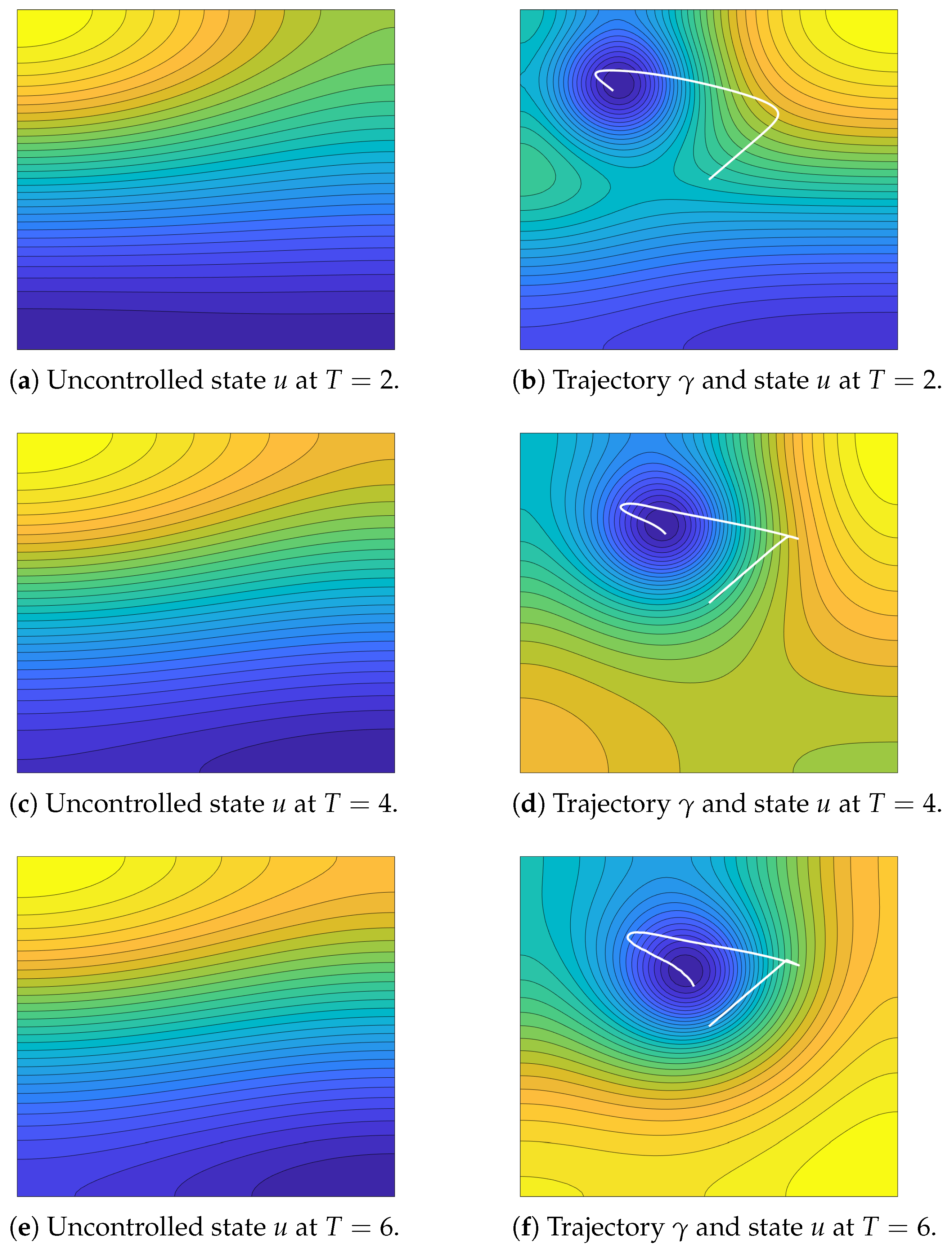
With no control, i.e., $b=0$ in (3), the solution evolves to a final state that is displayed in Figure 3a,c,e for $T=2,4$ and 6, respectively. In these figures, we observe that the mosquito population spreads and increases in $\Omega$. When we apply the control, due to the initial distribution of population, it is expected to obtain a solution that starts traveling in the direction of the nearest herd of mosquitos (the circle $B_2$ in the present case) and, then, changes course in the direction of the farthest herd ($B_1$). This is what is found in each case, as can be seen respectively in Figure 3b,d,f), where, besides the trajectories, the respective computed optimal states are also shown at the final time.

Table 2. Minimal and maximal values of the state u at $T=2,4,6$ for Figure 3.

Values for $T=2$	Figure 3a		Figure 3b
	$u_{min}$	$u_{max}$	$u_{min}$	$u_{max}$
	1.6517	8.3723	0.8906	3.4263
Values for $T=4$	Values for Figure 3c		Values for Figure 3d
	$u_{min}$	$u_{max}$	$u_{min}$	$u_{max}$
	24.0696	46.0825	2.9007	13.5890
Values for $T=6$	Values for Figure 3e		Values for Figure 3f
	$u_{min}$	$u_{max}$	$u_{min}$	$u_{max}$
	229.9722	305.1255	16.3627	77.1129

reports the minimal and maximal values of the control u in all cases depicted in Figure 3;

Table 3. Number of outer iterations (o.i.) and cost for each final time T, time subintervals N and meshes.

N	Mesh	$\mathit{T}=2$		$\mathit{T}=4$		$\mathit{T}=6$
		o.i.	Cost	o.i.	Cost	o.i.	Cost
	$20\times 20$	10	72.2095	8	923.973	12	34,349.7
50	$40\times 40$	11	109.81	10	1603.25	11	65,883.5
	$80\times 80$	11	117.87	10	1765.48	11	73,208.5
	$20\times 20$	9	72.1707	8	828.703	12	25,471.3
100	$40\times 40$	11	110.059	11	1426.18	11	48,688.7
	$80\times 80$	11	118.189	11	1566.38	11	54,065
	$20\times 20$	9	72.0812	8	816.119	11	22,673.7
200	$40\times 40$	11	110.172	9	1398.03	11	42,226.1
	$80\times 80$	11	118.333	11	1516.09	11	46,869.8

presents the required number of outer iterations and the obtained values of the cost functional F for the three considered meshes.

From the results in Table 3, we can observe that, for $T=2,4$, the change in the cost is lower to 4% for the third mesh and $N=200$. For this reason, we select these parameters to perform the simulations in the following sections. To keep the computational cost at a reasonable level, we also use the same parameters for $T=6$, where the relative change is about 13%.

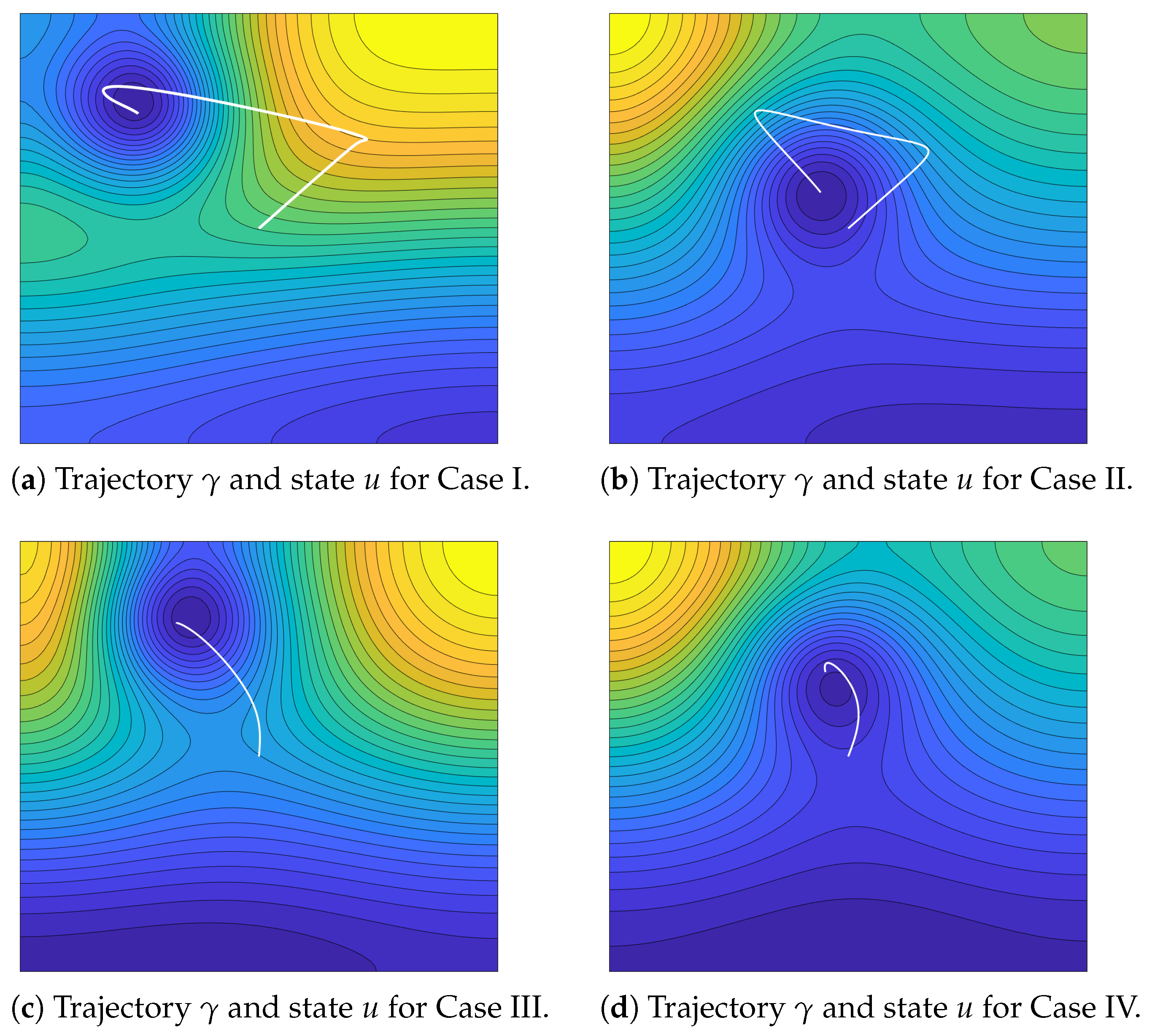
7.2. Influence of the Functional Weights

In this section, we study the influence of the functional weights. As in the previous section, we take $a(x,t)\equiv 1.0$.

Table 4. Number of outer iterations (o.i.) and cost for three final times T and four cases.

				$\mathit{T}=2$		$\mathit{T}=4$		$\mathit{T}=6$
	${\mathit{\mu }}_0$	${\mathit{\mu }}_1$	${\mathit{\mu }}_2$	o.i.	Cost	o.i.	Cost	o.i.	Cost
Case I	1	1	10	12	799.843	11	14,175.4	11	467,884
Case II	10	1	1	11	157.0	11	1589.28	11	46,938.6
Case III	1	10	1	8	179.831	10	1969.46	11	47,592.8
Case IV	10	10	1	5	201.137	10	2043.81	11	47,662.2

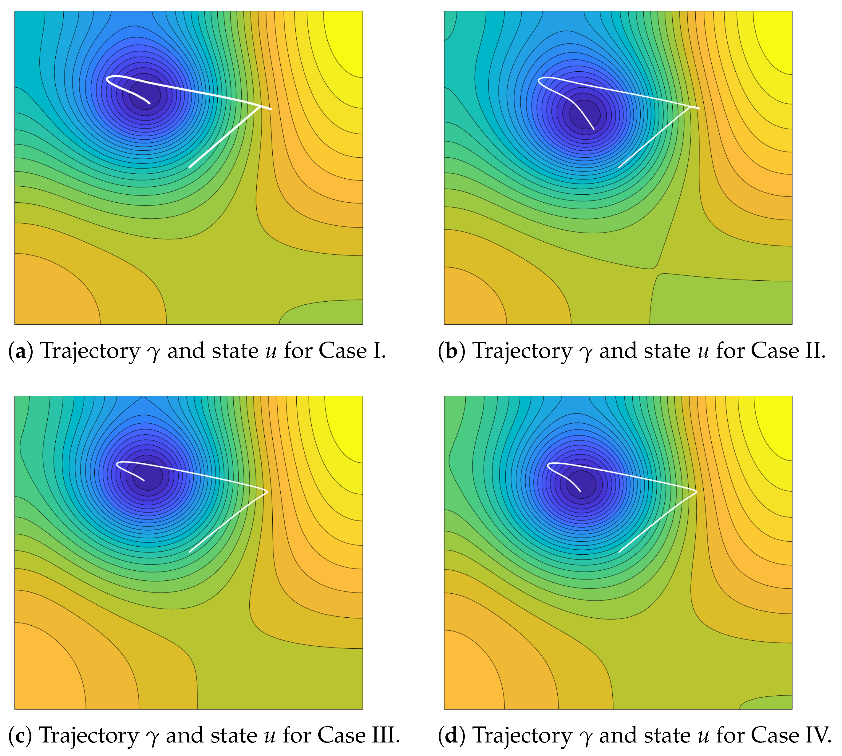
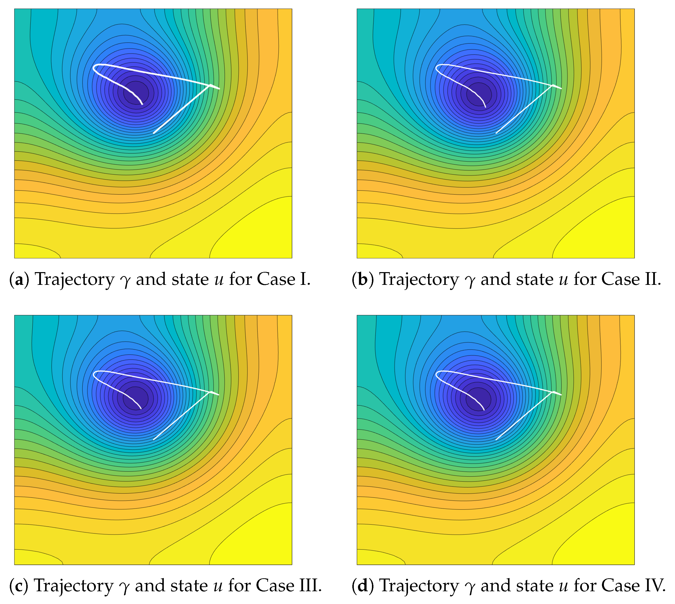
presents the required number of outer iterations, and the values of the cost functional in four cases I, II, III, and IV for three values of the final time: $T=2,4$, and 6. Calculations were made by using $N=200$ time steps and the third spatial mesh of Table 1.

From the results in Table 4, we see that the cost is larger in case I for small T. This seems to indicate that, when we assign major relevance to the remaining population, short time operations are not satisfactory. For larger T, the device cost becomes more important. We see, however, that, as T grows, the costs have a tendency to equalize (and the particular values of the ${\mu }_i$ seem to lose relevance).

Figure 4, Figure 5 and Figure 6 depict the trajectories and states u, respectively, at $T=2,4,6$ for all cases described in Table 4. The minimal and maximal values of the mosquito population u for each case are reported in

Table 5. Minimal and maximal values of the controlled state u at $T=2,4,6$ for cases I, II, III, and IV depicted in Figure 4, Figure 5 and Figure 6.

	Values for $\mathit{T}=2$		Values for $\mathit{T}=4$		Values for $\mathit{T}=6$
	Figure 4		Figure 5		Figure 6
	${\mathit{u}}_{\mathbf{min}}$	${\mathit{u}}_{\mathbf{max}}$	${\mathit{u}}_{\mathbf{min}}$	${\mathit{u}}_{\mathbf{max}}$	${\mathit{u}}_{\mathbf{min}}$	${\mathit{u}}_{\mathbf{max}}$
(a)	0.7468	2.9680	2.8730	13.5205	16.3729	77.1137
(b)	0.8214	4.9817	3.0829	13.5843	16.5243	77.0914
(c)	1.2411	4.7836	3.2204	14.2664	16.2753	77.1378
(d)	1.1635	6.6453	3.2603	14.2821	16.3462	77.1164

.

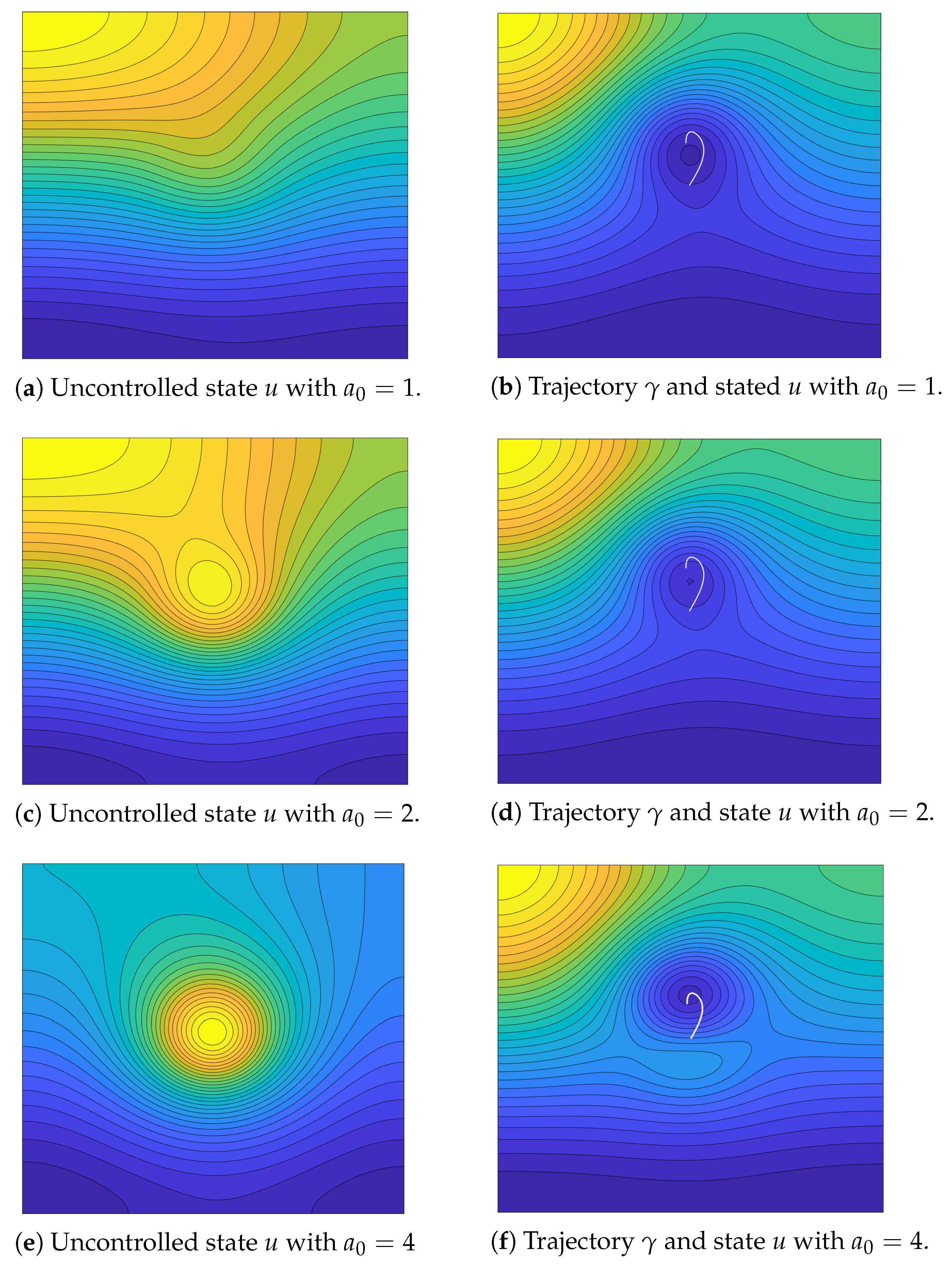
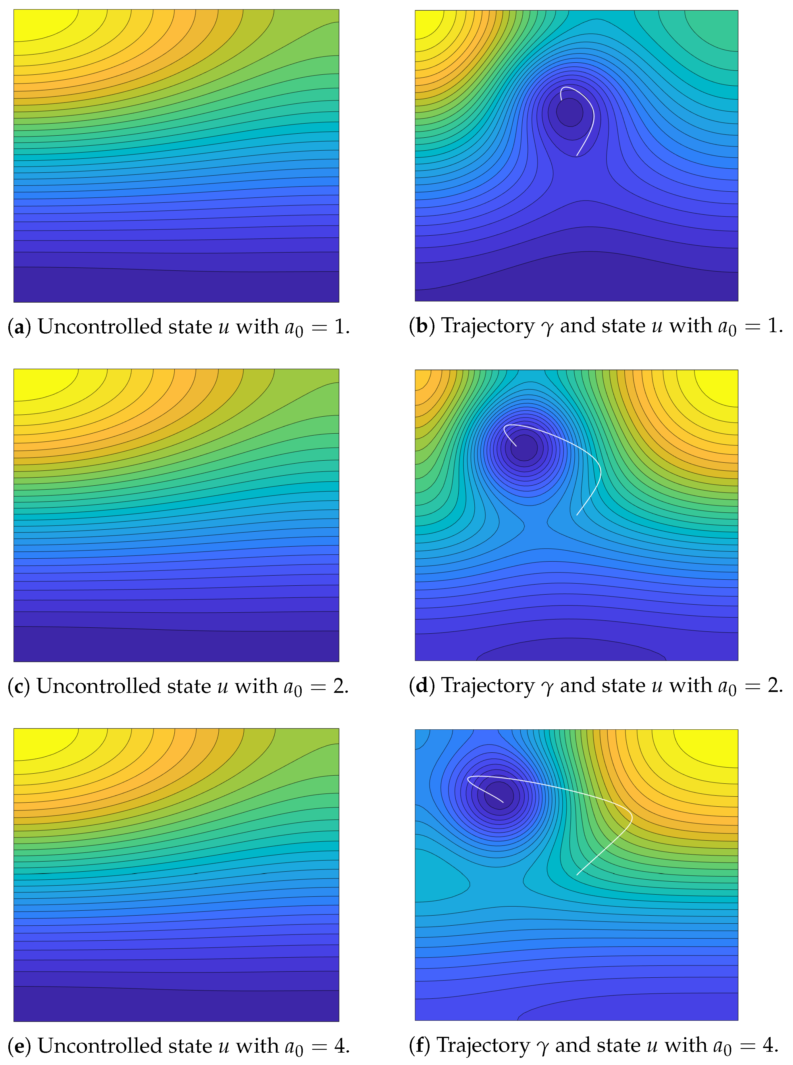
7.3. Two Examples with $a(·,·)$ Variable

In this section, we present the calculations obtained by considering the following two different definitions of the function a:

$$\begin{array}{ccc}\hfill a(x,t)& =& a_{0}max\left\{1-\sqrt{x^2+y^2},0\right\},\hfill \end{array}$$

(40)

$$\begin{array}{ccc}\hfill a(x,t)& =& a_{0}max\left\{1-t,0\right\}.\hfill \end{array}$$

(41)

with $a_0$ a positive constant associated with the proliferation velocity of the insect population. With these choices, we will study separately the influence of a in the spatial and time behavior of the state u and the control $\gamma$.

Calculations were carried out by considering $T=2$ with $N=200$ time steps, the third spatial mesh of Table 1 and the following values for $a_0$, and the weights of the functional F:

$$a_0=1,2,4,{\mu }_0={\mu }_1={\mu }_2=1.$$

Table 6. Number of outer iterations (o.i.) and values of the cost functional.

${\mathit{a}}_0$	$\mathit{a}(\mathit{x},\mathit{t})={\mathit{a}}_{0}max\left\{1-\sqrt{{\mathit{x}}^2+{\mathit{y}}^2},0\right\}$		$\mathit{a}(\mathit{x},\mathit{t})={\mathit{a}}_{0}max\left\{1-\mathit{t},0\right\}$
	o.i.	Cost	o.i.	Cost
1	4	28.2127	5	50.0751
2	3	28.5942	13	92.2256
4	3	29.4916	12	350.886

details the values of the number of outer iterations and the respective values of the cost functional in the case of $a(x,t)$ defined in (40) and (41) by considering three different values of $a_0$.

Figure 7 depicts the uncontrolled state, the controlled state, and the respective trajectory $\gamma$ for $T=2$ in the case of $a(x,t)$ defined in (40) by considering three different values of $a_0$: 1 (Figure 7a,b), 2 (Figure 7c,d), and 4 (Figure 7e,f). We observe that the optimal control trajectories are qualitatively similar in all cases and stay close to the initial point. This is because the non-zero values of a (where the insects proliferate) depend on the spatial coordinate and are located in the unit ball centered at this point.

Figure 8 depicts the uncontrolled state, the controlled state, and the respective trajectory $\gamma$ for $T=2$ in the case of $a(x,t)$ defined in (41) by considering three different values of $a_0$: 1 (Figure 8a,b), 2 (Figure 8c,d), and 4 (Figure 8e,f). In these cases, we can observe the influence of the time coordinate t: the length of the trajectory $\gamma$ increases when the value of $a_0$ does, giving a similar behavior for the case $a=1$ studied in Section 7.1.

The respective minimal and maximal values of the uncontrolled and controlled states corresponding to Figure 7 and Figure 8 are reported in

Table 7. Minimal and maximal values of the state u at $T=2$ for Figure 7 and Figure 8.

	Values for Figure 7		Values for Figure 8
	${\mathit{u}}_{\mathbf{min}}$	${\mathit{u}}_{\mathbf{max}}$	${\mathit{u}}_{\mathbf{min}}$	${\mathit{u}}_{\mathbf{max}}$
(a)	0.2341	1.1472	0.3595	1.8495
(b)	0.1579	0.9652	0.2517	1.4524
(c)	0.2547	1.1726	0.5950	3.0458
(d)	0.1678	0.9859	0.3769	1.5651
(e)	0.3181	2.3765	1.6465	8.3448
(f)	0.1982	1.0071	0.8043	3.6763

. The influence of the control $\gamma$ on the state u by decreasing their minimal and maximal values is clearly observed.

8. Conclusions

We have performed a rigorous analysis of an optimal control problem concerning the spreading of mosquito populations; the optimality conditions have been used to devise a suitable numerical scheme and compute an optimal trajectory.

The success in completing these tasks with the help of appropriate theoretical and numerical tools seems to indicate that a similar analysis can be performed in other more complex cases. Thus, it can be more natural to consider, instead of (2), the cost functional

$${\displaystyle F\left(\gamma \right):={\mu }_0{\int }_0^T|\gamma |dt+{\mu }_1{\int }_0^T|\dot{\gamma }|dt+{\mu }_2\int {\int }_{Q}udxdt.}$$

Indeed, in this functional, the three terms can be respectively viewed as measures of the true length of the path traveled by the device, the total fuel needed in the process, and the total mosquito population along $(0,T)$. The $L^1$ norms of $\gamma$, $\dot{\gamma }$ and u represent quantities more adequate to the model, although the analysis of the corresponding control problem is more involved.

Other realistic situations can also be taken into account. For instance, a very interesting setup appears when there are obstacles to the admissible trajectories. In addition, instead of the Malthusian growth rate for the mosquito population assumed in the present work, we could assume a Verhustian or Gomperzian growth rate. The corresponding models and their associated control problems are being investigated at present.