A Simple Analytical Method for Estimation of the Five-Parameter Model: Second-Order with Zero Plus Time Delay

Abstract

Process models play an important role in the process industry. They are used for simulation purposes, quality control, fault detection, and control design. Many researchers have been engaged in model identification. However, it is difficult to find an analytical identification method that provides a good model and requires a relatively simple experiment. This is the advantage of the method of moments. In this paper, an analytical method based on the measurement of the process moments (characteristic areas) is proposed, to identify the five-parameter model (second-order process with zero plus time delay) from either the closed-loop or open-loop time responses of the process (in the time-domain), or the general-order transfer function with time delay (in the frequency-domain). The only parameter required by the user is the type of process (minimum phase or non-minimum phase process), which in practice can be easily determined from the time response of the process. The method can also be used to reduce the higher-order process model. The proposed identification method was tested on several illustrative examples, and compared to other identification methods. The comparison with existing methods showed the superiority of the proposed method. Moreover, the tests confirmed that the algorithm of the proposed method works properly for a wide family of process models, even in the presence of moderate process noise.

1. Introduction

A process model is a set of equations that describe the input and output relationships of the actual process. Process models can be derived for a variety of purposes, such as process simulation, fault detection, or control system design. The performance of the control system usually correlates with the quality and complexity of the process model. However, a complex process model usually leads to a complex controller structure, higher sensitivity of the control loop, and lower robustness to process parameter perturbations [1].

The goal of a control system is to force the control system to behave with the desired dynamics. The success of this goal often depends on the existence of an accurate mathematical model of the process [1,2,3]. According to [4], “the primary goal of system or process identification is to determine a model that matches the performance of the system or process being identified”. Models are used for simulation purposes, quality control, fault detection, and control design [1,5]. According to [5], “models can be used to simulate the expected process behaviour with a proposed control system”. Moreover, models are often “embedded” in the controller itself; in fact, the controller may use a process model to anticipate the effect of a control action”. They also play an important role when real-time system experiments are dangerous or costly [1,5]. In this paper, we focus on linear time-invariant (LTI) single-input single-output (SISO) processes.

The model parameters are identified by feeding a set of input signals into the system. Then, the response of the system is acquired by taking measurements with appropriate sensors that are affected by the measurement noise [1,2,4,5]. Different input data signals can be used, such as step, pulse, a square wave, sine, and pseudorandom binary sequences (PRBS). To prevent the process output from drifting too far from the setpoint, process identification can also be performed in a closed-loop configuration, although this is not possible in all cases. According to [6], “for safety and economic reasons, many industrial processes of the type integrating and unstable processes are not permitted to run in an open-loop manner”.

Based on the information obtained, identification methods can be divided into time-domain and frequency-domain methods [2,4]. A comprehensive review of identification methods was presented in [6,7].

The most common frequency-domain identification method is a relay feedback identification method [2,8,9]. Several variants of relay identification methods have been proposed in the literature [9,10,11,12,13,14,15,16,17,18,19,20,21,22,23,24]. According to [6] and [7], they can be categorized into three main groups: describing function method, curve fitting approach, and frequency response estimation for model fitting. The advantage of relay feedback methods is that process identification is in a closed-loop configuration. Moreover, the relay identification solution that was proposed by Šekara and Mataušek [20] is implemented without breaking the control loop while the controller is running. Relay identification is widely used for controller tuning [9,10,13,21,23]. According to [22], “the success of relay feedback auto-tunes lines on the fact that it identifies one important point on the Nyquist curve: the point at the crossover frequency (ultimate frequency)”. Moreover, relay identification has been improved with a shifting method [11,12,13,16,24], which is still based on biased relay feedback. This shifting method can find up to three points on the frequency characteristics [16]. Frequency identification methods based on the input step response of the process usually apply a two-step identification procedure: the estimation of the process response in two frequency ranges [25]. Some of the less used frequency-domain methods use sinusoidal or impulse process input signals. The sinusoidal test is usually time consuming, and the impulse test is not suitable for nonlinear systems [6].

The step test is the most commonly used method in the time-domain because of its simplicity. It can be further divided into the model-fitting approach, and the time integral approach [6,25]. Model fitting techniques roughly estimate the process model, such as the first-order plus time delay (FOTD) model or the second-order plus time delay (SOPTD) model, based on two-point fitting [26,27,28]. According to [3,28], for the purpose of controller tuning, the lower order model can effectively describe the higher-order linear process (HO). Later, the three-point fitting was proposed [29,30,31,32], as well as a method for obtaining the HO model with time delay [33], for stable processes with underdamped responses. To improve the identification accuracy and robustness to high-frequency noise, the time integral approach was proposed [28,34,35,36]. In [35], it was shown by benchmark examples that the time integral algorithm improves the identification accuracy and robustness to high-frequency noise, compared to that of other stage identification methods. At this point, classical identification methods for estimating ARMAX models using regression should also be mentioned [37].

Another method for process identification in the time-domain is the method of moments [38,39,40]. This method uses successive (multiple) integrations of the input and output time responses of the process [39] to obtain so-called moments or “characteristic areas” of the process. The characteristic areas can be computed from any change of the process steady-state in the closed-loop or open-loop configuration (time-domain approach). Moreover, it has been shown in [41,42] that the characteristic areas can also be obtained from integrating processes, and that the characteristic areas can be easily used for model reduction.

On the other hand, the same characteristic areas can also be obtained from any process transfer function with a time delay (frequency-domain approach) [43], and conversely, SOPDT (four-parameter model) can be calculated analytically from the moments or characteristic areas, as shown in [28,44]. However, since the SOPDT model does not contain a zero, it is not suitable for certain applications; see, for example, a calculation of higher-order reference filter parameters in [42].

In this paper, we propose a method to identify the five-parameter model from characteristic areas: the second-order process with zero plus time delay. This method can also be used to reduce the HO process model, to obtain the process model from the original infinite order model (e.g., heat transfer), or to obtain the process model containing the sum of the different process delays. Note that the proposed identification method is not suitable for unstable processes.

The content of this paper is organized as follows. First, a method for a nonparametric identification of the process is presented. In Section 3, the proposed method for a second-order identification of the process with zero plus time delay (five-parameter model) is presented. In Section 4, the proposed identification method is tested in a frequency- and time-domain and compared with other identification methods. Additionally, sensitivity to the process noise was tested.

2. Characteristic Areas (Process Moments)

In this section, we present a method for process identification, based on measured or calculated moments (characteristic areas) of the process [38,39,40]. As mentioned before, the characteristic areas can be calculated from an arbitrary change in the steady-state of the process, in the closed-loop or open-loop configuration (time-domain approach). On the other hand, the characteristic areas can also be obtained from the arbitrary process transfer function with a time delay (frequency-domain approach). Both approaches are equivalent [42,43].

The process is represented by the next stable proportional transfer function:

$$G_{\mathrm{P}}\left(s\right)=K_{\mathrm{PR}}\frac{1+b_{1}s+b_2{s}^2+\cdots +b_{\mathrm{m}}{s}^m}{1+a_{1}s+a_2{s}^2+\cdots +a_{\mathrm{n}}{s}^n}{e}^{-s{T}_{\mathrm{delay}}},$$

(1)

where T_delay is the process time delay, and parameters a₁ to a_n and b₁ to b_m are the dynamic process parameters. To simplify the further derivation, the Function (1) can be developed into an infinite Taylor series around s = 0:

$$G_{\mathrm{P}}\left(s\right)=G_{\mathrm{P}}\left(0\right)+\frac{s}{1!}{\left.\frac{d{G}_{\mathrm{P}}\left(s\right)}{ds}\right|}_{s=0}+\frac{s^2}{2!}{\left.\frac{d^2{G}_{\mathrm{P}}\left(s\right)}{d{s}^2}\right|}_{s=0}+\cdots =A_0-A_{1}s+A_2{s}^2-A_3{s}^3+\cdots ,$$

(2)

where A_i represents the moments (characteristic areas) of the Function (1). By solving (2), the characteristic areas can be expressed by the parameters of the process transfer function (1):

$$\begin{gathered} A_0=K_{\mathrm{PR}} \\ {A}_1=K_{\mathrm{PR}}\left(a_1-b_1+T_{\mathrm{delay}}\right) \\ {A}_2=K_{\mathrm{PR}}\left(b_2-a_2-T_{\mathrm{delay}}{b}_1+\frac{T_{\mathrm{delay}}{}^2}{2!}\right)+A_1{a}_1 \\ {A}_3=K_{\mathrm{PR}}\left(a_3-b_3+T_{\mathrm{delay}}{b}_2-\frac{T_{\mathrm{delay}}{}^2{b}_1}{2!}+\frac{T_{\mathrm{delay}}{}^3}{3!}\right)+A_2{a}_1-A_1{a}_2 \\ {A}_4=K_{\mathrm{PR}}\left(-a_4+b_4-T_{\mathrm{delay}}{b}_3+\frac{T_{\mathrm{delay}}{}^2{b}_2}{2!}-\frac{T_{\mathrm{delay}}{}^3{b}_1}{3!}+\frac{T_{\mathrm{delay}}{}^4}{4!}\right)+ \\ {A}_3{a}_1-A_2{a}_2+A_1{a}_3 \\ ⋮ \\ {A}_{\mathrm{k}}=K_{\mathrm{PR}}\left({\left(-1\right)}^{k+1}\left(a_{\mathrm{k}}-b_{\mathrm{k}}\right)+{\displaystyle \sum }_{i=1}^k{\left(-1\right)}^{k+i}\frac{T_{\mathrm{delay}}{}^i{b}_{\mathrm{k}-i}}{i!}\right)+ \\ {{\displaystyle \sum }}_{i=1}^{k-1}{\left(-1\right)}^{k+i-1}{A}_{\mathrm{i}}{a}_{\mathrm{k}-i}. \end{gathered}$$

(3)

As can be seen above, the characteristic areas can be calculated directly and analytically from the process transfer function [42,43].

In addition, the characteristic areas can also be calculated directly from the time response of the process. This is achieved by changing the steady-state of the process (by changing the process input signal) and calculating subsequent (multiple) integrations of the process input (u(t)) and output(y(t)) time responses:

$$\begin{array}{cc}{u}_0=\frac{u\left(t\right)-u\left(0\right)}{\Delta U}& y_0\left(t\right)=\frac{y\left(t\right)-y\left(0\right)}{\Delta U}\\ I_{U1}\left(t\right)=\underset{0}{\overset{t}{{\displaystyle \int }}}{u}_0\left(\tau \right)d\tau & I_{Y1}\left(t\right)=\underset{0}{\overset{t}{{\displaystyle \int }}}{y}_0\left(\tau \right)d\tau \\ I_{U2}\left(t\right)=\underset{0}{\overset{t}{{\displaystyle \int }}}{I}_{U1}\left(\tau \right)d\tau & I_{Y2}\left(t\right)=\underset{0}{\overset{t}{{\displaystyle \int }}}{I}_{Y1}\left(\tau \right)d\tau \\ ⋮& ⋮,\end{array}$$

(4)

where u₀ represents the normalized process input signal, y₀ the normalized process output signal and

$$\Delta U=u\left(\infty \right)-u\left(0\right).$$

(5)

The characteristics areas (time integrals) can be calculated as follows [43]:

$$\begin{array}{ll}{A}_0& =y_0\left(\infty \right); y_1=A_0{I}_{U1}\left(t\right)-I_{Y1}\left(t\right)\\ A_1& =y_1\left(\infty \right); y_2=A_1{I}_{U1}\left(t\right)-A_0{I}_{U2}\left(t\right)+I_{Y2}\left(t\right)\\ A_2& =y_2\left(\infty \right); y_3=A_2{I}_{U1}\left(t\right)-A_1{I}_{U2}\left(t\right)+A_0{I}_{U3}\left(t\right)-I_{Y3}\left(t\right)\\ & ⋮\end{array}$$

(6)

Note that $\dot{y}\left(0\right)=\ddot{y}\left(0\right)=\stackrel{⃛}{y}\left(0\right)=\cdots =\dot{y}\left(\infty \right)=\ddot{y}\left(\infty \right)=\stackrel{⃛}{y}\left(\infty \right)=\cdots =0$ and that A₀ is equal to the steady-state gain of the process, K_PR. In practice, the computation of Expressions (4) can be terminated when the process has settled down. Note that the Expressions (4) can also be computed recursively, and that the characteristic areas can be obtained from any change of the process steady-state [42,43]. A more detailed procedure, including some practical guidelines for computing characteristic areas from the process input and output time signals, even in noisy environments, is given in [45].

Note that the characteristic areas can also be obtained for integrating processes [42]. In this case, Expression (4) is changed to:

$$\begin{gathered} \begin{array}{ll}{u}_0=\frac{u\left(t\right)-u\left(0\right)}{\Delta U} \\ {I}_{U1}\left(t\right)=\underset{0}{\overset{t}{{\displaystyle \int }}}{u}_0\left(\tau \right)d\tau \\ {I}_{U2}\left(t\right)=\underset{0}{\overset{t}{{\displaystyle \int }}}{I}_{U1}\left(\tau \right)d\tau \\ ⋮& I_{Y1}\left(t\right)=\frac{y\left(t\right)-y\left(0\right)-\dot{y}\left(0\right)\cdot t}{\Delta U} \\ {I}_{Y2}\left(t\right)=\underset{0}{\overset{t}{{\displaystyle \int }}}{I}_{Y1}\left(\tau \right)d\tau \\ ⋮\end{array} \end{gathered}$$

(7)

To save the reader effort and time, all MATLAB files that are needed to implement the calculation of the characteristic areas are available online [46].

3. Model Identification

In [28], it was shown that higher-order systems can also be successfully approximated by the second-order process model with time delay (four-parameter model):

$$G_{\mathrm{M}}\left(s\right)=\frac{K_{\mathrm{M}}{e}^{-T_{\mathrm{dm}}s}}{1+a_{1\mathrm{m}}s+a_{2\mathrm{m}}{s}^2},$$

(8)

where T_dm and K_M represent the process time delay and the steady-state gain, respectively. a_1m and a_2m are the corresponding dynamic parameters. Vrečko et al. [44] have shown that all parameters of the Process model (8) can be calculated analytically from the Expressions (3). Therefore, the process model can be obtained directly from the characteristic areas.

As explained earlier, a model without zero is not suitable for certain applications. Therefore, the modelling method proposed by Vrečko et al. [44] is extended here. The chosen process model is a second-order process with a zero and a time delay

$$G_{\mathrm{M}}\left(s\right)=\frac{K_{\mathrm{M}}\left(1+b_{1\mathrm{m}}s\right)e^{-T_{\mathrm{dm}}s}}{1+a_{1\mathrm{m}}s+a_{2\mathrm{m}}{s}^2},$$

(9)

where b_1m represents the process zero.

In order to express the parameters of the Model (9), in terms of the characteristic areas A₀–A₄, Expression (9) is inserted into Expressions (3). The following result is obtained:

$$\begin{gathered} A_0=K_{\mathrm{M}} \\ {A}_1=K_{\mathrm{M}}\left(a_1-b_1+T_{\mathrm{dm}}\right) \\ {A}_2=K_{\mathrm{M}}\left(-a_2-T_{\mathrm{dm}}{b}_1+\frac{T_{\mathrm{dm}}{}^2}{2!}\right)+A_1{a}_1. \\ {A}_3=K_{\mathrm{M}}\left(-\frac{T_{\mathrm{dm}}{}^2{b}_1}{2!}+\frac{T_{\mathrm{dm}}{}^3}{3!}\right)+A_2{a}_1-A_1{a}_2 \\ {A}_4=K_{\mathrm{M}}\left(-\frac{T_{\mathrm{dm}}{}^3{b}_1}{3!}+\frac{T_{\mathrm{dm}}{}^4}{4!}\right)+A_3{a}_1-A_2{a}_2 \end{gathered}$$

(10)

As can be seen from Expressions (10), the characteristic area A₀ is equal to the steady-state process gain. The remaining process model parameters can then be calculated directly from Expressions (10). The time delay can be calculated from the following sixth-order polynomial:

$$\alpha T_{\mathrm{dm}}{}^6+\beta T_{\mathrm{dm}}{}^5+\gamma T_{\mathrm{dm}}{}^4+\delta T_{\mathrm{dm}}{}^3+\mathsf{\epsilon }{T}_{\mathrm{dm}}{}^2+\vartheta T_{\mathrm{dm}}+\mathsf{\rho }=0,$$

(11)

where

$$\begin{array}{ll}\mathsf{\alpha }& =A_0{}^3,\\ \beta & =-6A_1{A}_0{}^2,\\ \gamma & =6\left(-A_2{A}_0{}^2+3A_1{}^2{A}_0\right),\\ \delta & =24\left(A_3{A}_0{}^2-A_1{}^3\right),\\ \epsilon & =72\left(A_4{A}_0{}^2+A_2{A}_1{}^2-2A_3{A}_1{A}_0\right),\\ \vartheta & =144\left(A_3{A}_1{}^2-A_2{}^2{A}_1-A_4{A}_1{A}_0+A_3{A}_2{A}_0\right),\\ \rho & =144\left(A_4{A}_1{}^2+A_3{}^2{A}_0+A_2{}^3-A_4{A}_2{A}_0-2A_3{A}_2{A}_1\right).\end{array}$$

(12)

Expression (11) has six solutions for the time delay T_dm, which can be real or complex. The selection of the appropriate T_dm values will be shown later. Then, the zero of the process model can be calculated from the following expression:

$$b_{1\mathrm{m}}=\frac{A_0{}^3{T}_{\mathrm{dm}}{}^3-3A_1{A}_0{}^2{T}_{\mathrm{dm}}{}^2-6A_2{A}_0{}^2{T}_{\mathrm{dm}}-6A_3{A}_0{}^2+6A_1{}^2{A}_0{T}_{\mathrm{dm}}+12A_2{A}_1{A}_0-6A_1{}^3}{3\left(A_0{}^3{T}_{\mathrm{dm}}{}^2-2A_1{A}_0{}^2{T}_{\mathrm{dm}}-2A_2{A}_0{}^2+2A_1{}^2{A}_0\right)},$$

(13)

and the denominator’s parameters a_1m and a_2m from the following expressions:

$$\begin{gathered} a_{1\mathrm{m}}=\frac{A_1}{A_0}+b_{1\mathrm{m}}-T_{\mathrm{dm}}, \\ {a}_{2\mathrm{m}}=-\frac{A_2}{A_0}+\frac{T_{\mathrm{dm}}{}^2}{2}-b_{1\mathrm{m}}{T}_{\mathrm{dm}}+\frac{A_1\left(A_1+A_0{b}_{1\mathrm{m}}-A_0{T}_{\mathrm{dm}}\right)}{A_0{}^2}. \end{gathered}$$

(14)

The flowchart for calculating the model parameters, according to the proposed model-fitting method, is shown in Figure 1.

At the beginning, the time delay T_dm0 (when the process model zero is fixed to b_1m = 0) is determined by blocks A–D. The value T_dm0 is used for decision making, and is calculated by block A from the following third-order polynomial [44]:

$$\frac{T_{\mathrm{d}m0}{}^3}{6}-\frac{T_{\mathrm{dm}0}{}^2{A}_1}{2A_0}+T_{\mathrm{dm}0}\left(\frac{A_1{}^2}{A_0{}^2}-\frac{A_2}{A_0}\right)-\frac{A_1{}^3}{A_0{}^3}+\frac{2A_1{A}_2}{A_0{}^2}+\frac{A_3}{A_0}=0.$$

(15)

Expression (15) has three solutions for T_dm0, which may be real or complex. The time delay must be real and non-negative to represent a feasible solution. These constraints can be expressed as follows:

$$\begin{array}{c}\Im \left(T_{\mathrm{dm}0}\right)=0\\ \Re \left(T_{\mathrm{dm}0}\right)\ge 0\end{array}.$$

(16)

The correct result is the smallest positive real number, resulting from blocks B and C. Condition D checks if the solution exists, otherwise, T_dm0 is set to 0.

Next, block E computes the time delay T_dm from Expressions (11) and (12). The time delay must be real and non-negative to represent a feasible solution. These constraints (block F) can be expressed as follows:

$$\begin{array}{c}\Im \left(T_{\mathrm{dm}}\right)=0\\ \Re \left(T_{\mathrm{dm}}\right)\ge 0\end{array}.$$

(17)

The condition G checks if the feasible solution(s) exist, otherwise T_dm = T_dm0 (calculated time delay for b_1m = 0). The model parameters b_1m, a_1m, and a_2m are calculated according to Expressions (13) and (14), as shown in block H.

The process model must be stable, i.e., a_1m and a_2m must be non-negative. These boundary conditions (block I) can be expressed as follows:

$$\begin{array}{c}{a}_{1\mathrm{m}}\ge 0\\ a_{2\mathrm{m}}\ge 0\end{array}.$$

(18)

If there are multiple solutions (block J), the appropriate solution is selected according to the process type (block K), i.e., for a minimum phase or non-minimum phase process. Note that the process type must be specified by the user beforehand. In the case of a minimum phase process, the correct solution is the one with T_dm ≥ T_dm0 and vice versa. These constraints can be expressed as follows:

$$\begin{array}{cc}{T}_{\mathrm{dm}}\ge T_{\mathrm{dm}0}& \mathrm{process}=\mathrm{minimum} \mathrm{phase}\\ T_{\mathrm{dm}}<T_{\mathrm{dm}0}& \mathrm{process}=\mathrm{non}-\mathrm{minimum} \mathrm{phase}\end{array}.$$

(19)

The final condition (block L) checks whether there is a matching solution. If the condition is satisfied, the loop is terminated. Otherwise, the algorithm sets T_dm = T_dm0 (time delay at b_1m = 0), and then blocks H–K are called again. Note that block L is called only once to avoid unwanted code loops.

As has been shown, the second-order process model (9) can be estimated from the characteristic areas, and the only parameter required by the user is the type of process (minimum phase or non-minimum phase process), which in practice can be easily obtained from the process time response. To save the reader effort and time, all MATLAB files that are required to implement the proposed identification method and calculate the process model parameters from the characteristic areas are available online [46].

4. Illustrative Examples

The proposed identification method was tested and compared with other identification methods. The calculation of the characteristic areas was performed either in the frequency-domain (directly from the process transfer function) or in the time-domain (from the process open-loop time response).

Two fitting criteria were used to evaluate the performance of the model identification. The step response difference was evaluated using the following time-domain criterion:

$$\mathrm{IAE}=\frac{{{\displaystyle \int }}_0^{\infty }\left|e\right|\left(t\right)dt}{\left|\max \left(y_{G_{\mathrm{P}}}\right)-\min \left(y_{G_{\mathrm{P}}}\right)\right|},$$

(20)

where e is the open-loop step response difference between the actual process ( $y_{G_{\mathrm{P}}}$) and the identified process model output signal ( $y_{G_{\mathrm{M}}}$):

$$e=y_{G_{\mathrm{P}}}-y_{G_{\mathrm{M}}}.$$

(21)

The frequency response error was evaluated using the following criterion:

$$\mathrm{ERR}=\underset{\omega \in \left[{\omega }_0,{\omega }_{\mathrm{c}}\right]}{\mathrm{mean}}\left\{\left|G_{\mathrm{P}}\left(j\omega \right)-G_{\mathrm{M}}\left(j\omega \right)\right|\right\},$$

(22)

where jω is the complex angular frequency. The lower (ω₀) and upper (ω_C) frequency bounds were selected to cover the process frequency response from around 0 to the frequency corresponding to ∠G_P(jω) = −180°. This is a common choice when the purpose of the process model is a controller design. The frequency points were chosen in geometric progression, as arithmetic progression would disproportionately favour higher frequency regions. Due to the geometric progression, ω₀ is not zero, but a relatively low frequency, defined by the following expression:

$${\omega }_0=\frac{A_0}{A_1}\times \frac{1}{100},$$

(23)

where the characteristic areas A₀ and A₁ are calculated from the actual process G_P(s). As already mentioned, the upper bound (cutoff) angular frequency ω_C is corresponding to ∠G_P(jω) = −180°. The frequency vector ω has been defined from ω₀ to ω_C with 10⁵ points per decade.

4.1. Model Identification from a General-Order Transfer Function with a Time Delay

In this subsection, the proposed identification method was tested in the frequency-domain, i.e., the characteristic areas are calculated from a process transfer function. For this purpose, the method was tested on the following family of the process models:

$$G_{\mathrm{P}1}\left(s\right)=\frac{\left(1+bs\right)e^{-T_{\mathrm{delay}}s}}{{\left(1+Ts\right)}^n},$$

(24)

where b, T_delay, T, and n represent the process numerator time constant, the time delay, the time constant, and the process order, respectively. The test experiments were performed for different values on all four parameters of the Process (24). The time constant T was calculated from the selected process order and time delay as follows:

$$T=\frac{1-T_{\mathrm{delay}}}{n}.$$

(25)

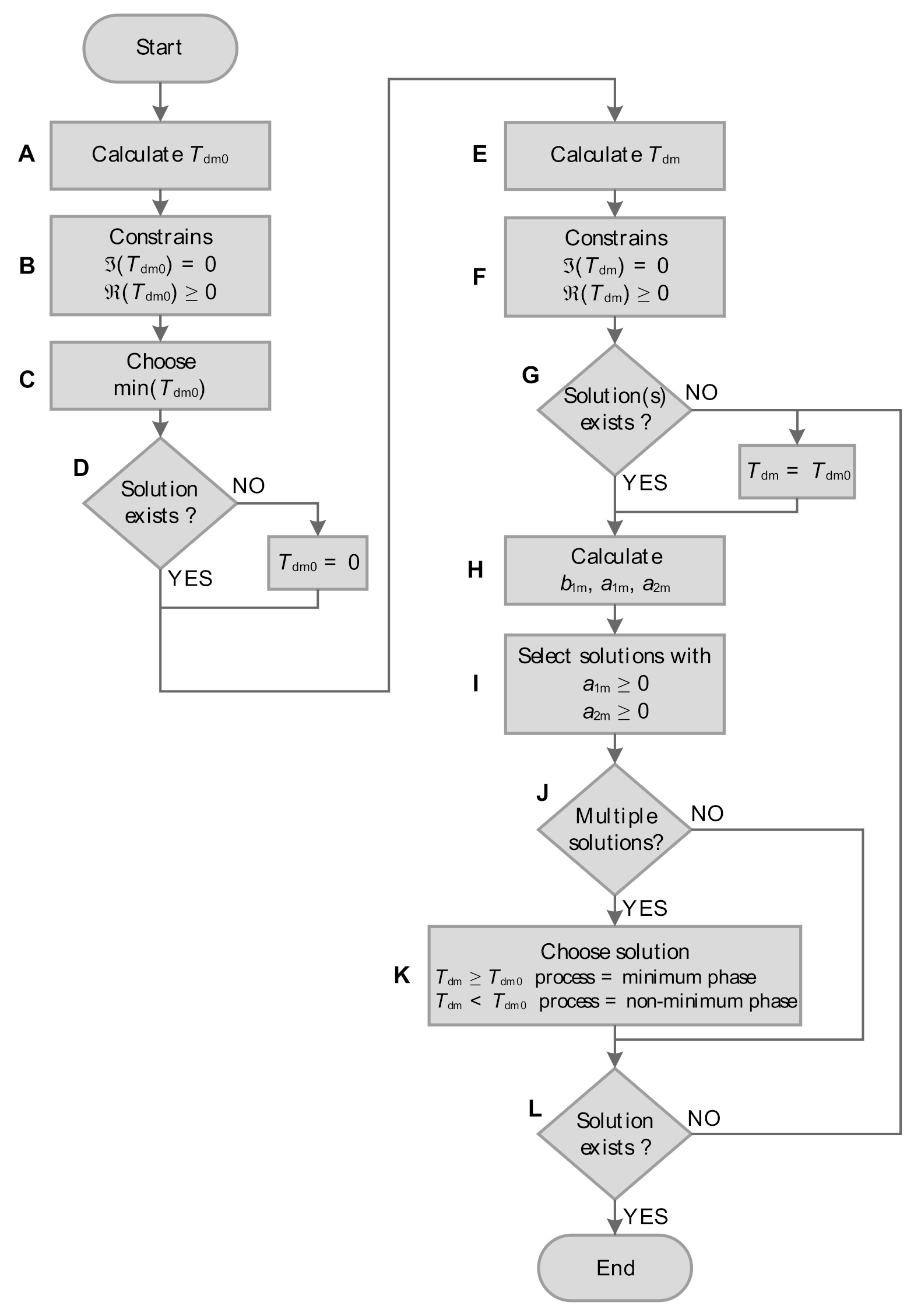
Expression (3) was used to calculate the characteristic areas from the transfer function of the Process (24). Then, the parameters of the Process model (9) were calculated from the characteristic areas, according to the flowchart shown in Figure 1.

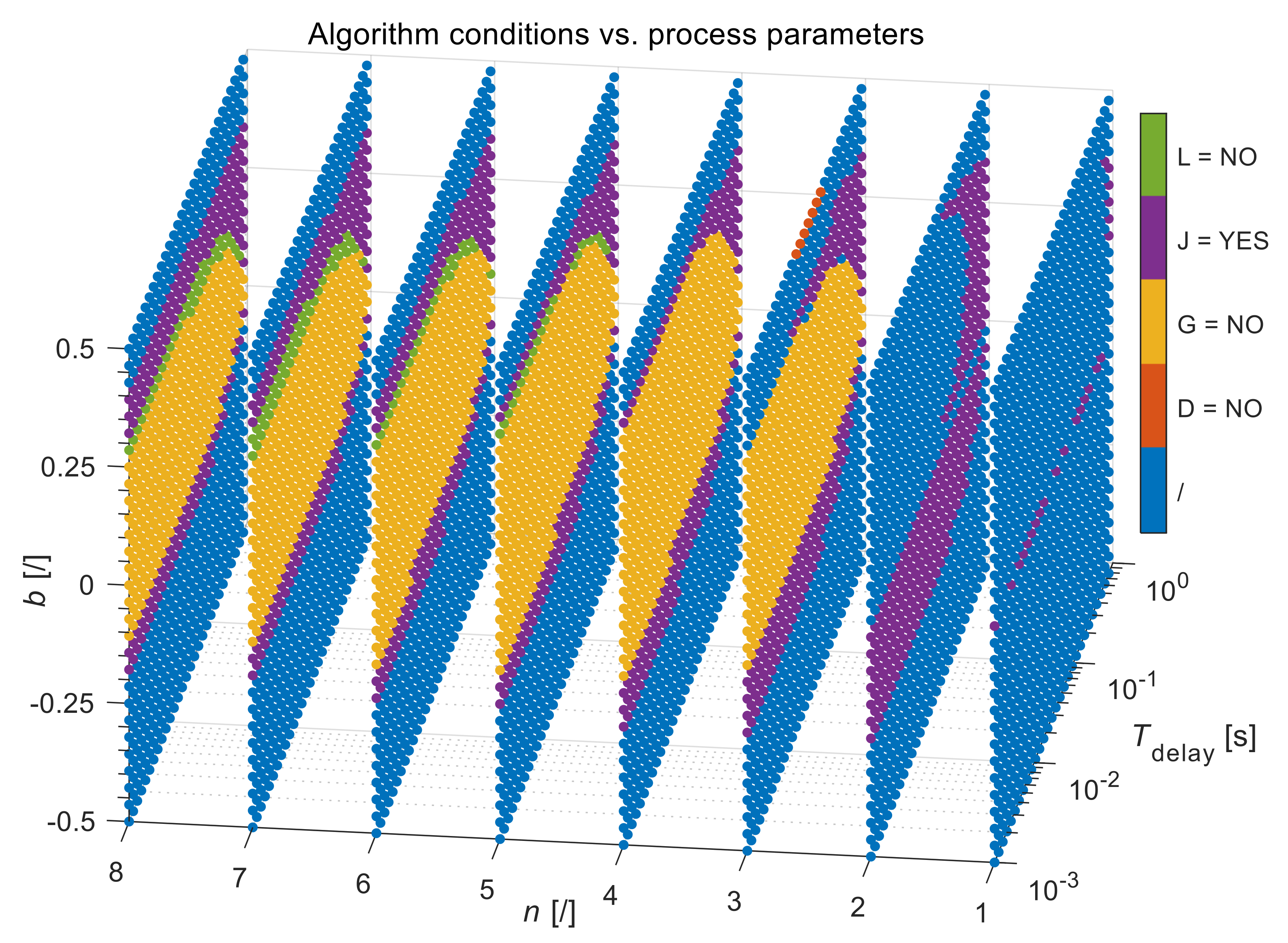
The actual flow of the algorithm in Figure 1 depends on the selection of the parameters in the Process (24). The results of all the conditions (rhomboid-shaped blocks in Figure 1) for a different selection of the process parameters (process zero, time delay, time constant, and process order) are shown in Figure 2. The conditions shown represent all the decisions made by the algorithm. For example, D = NO, means that the answer of block D in Figure 1 is NO (there is no real positive solution for the process model time delay T_dm0), G = NO means that there is no real positive solution for the process model time delay T_dm, J = YES means that there are multiple solutions for computing the dynamic process parameters a_1m and a_2m, and L = NO indicates that there are no solutions for the model parameters when T_dm is used, so in the next iteration T_dm = T_dm0. Note that for each process, only one of the conditions shown in the figure is met so that there is no overlap.

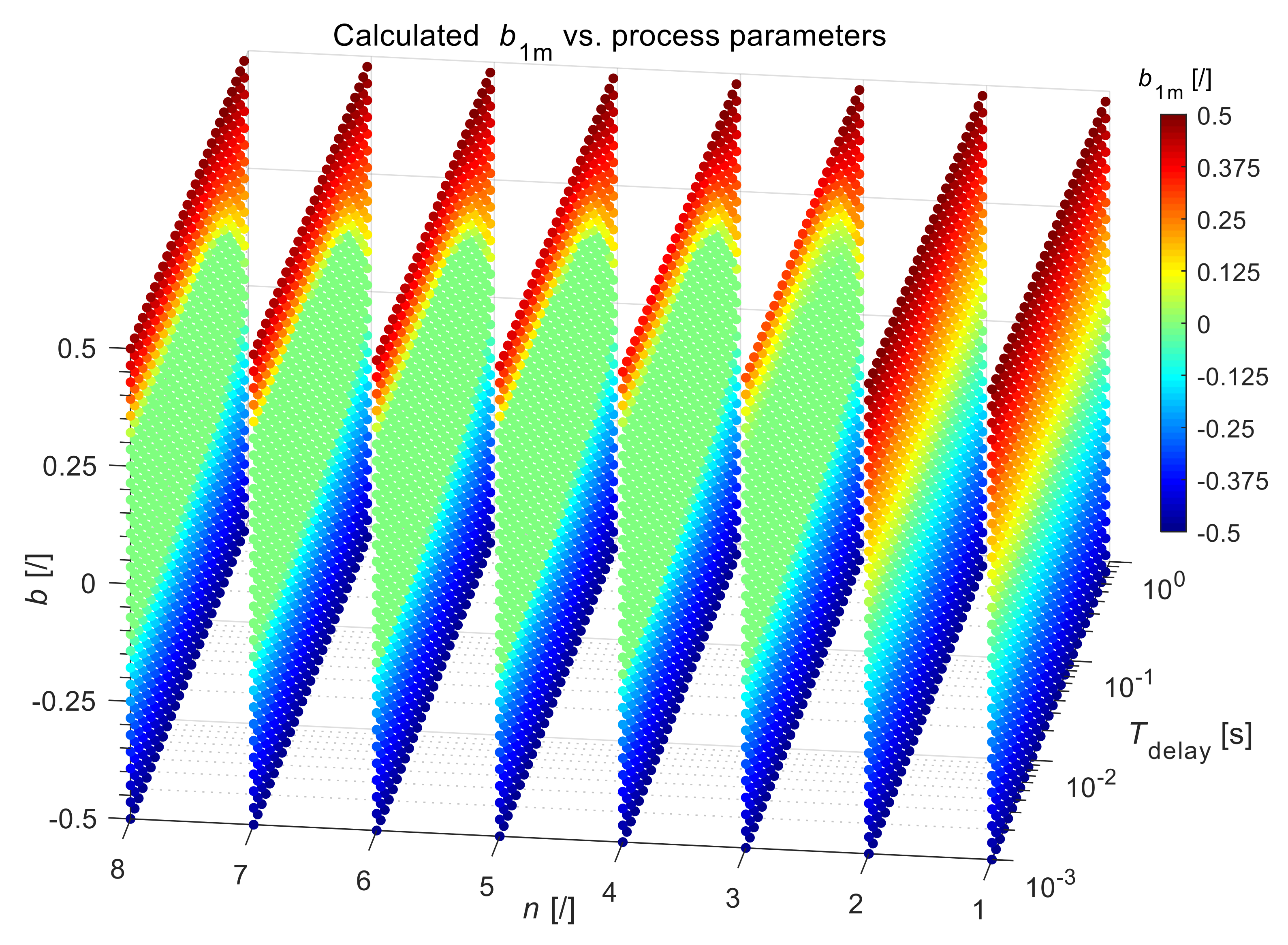
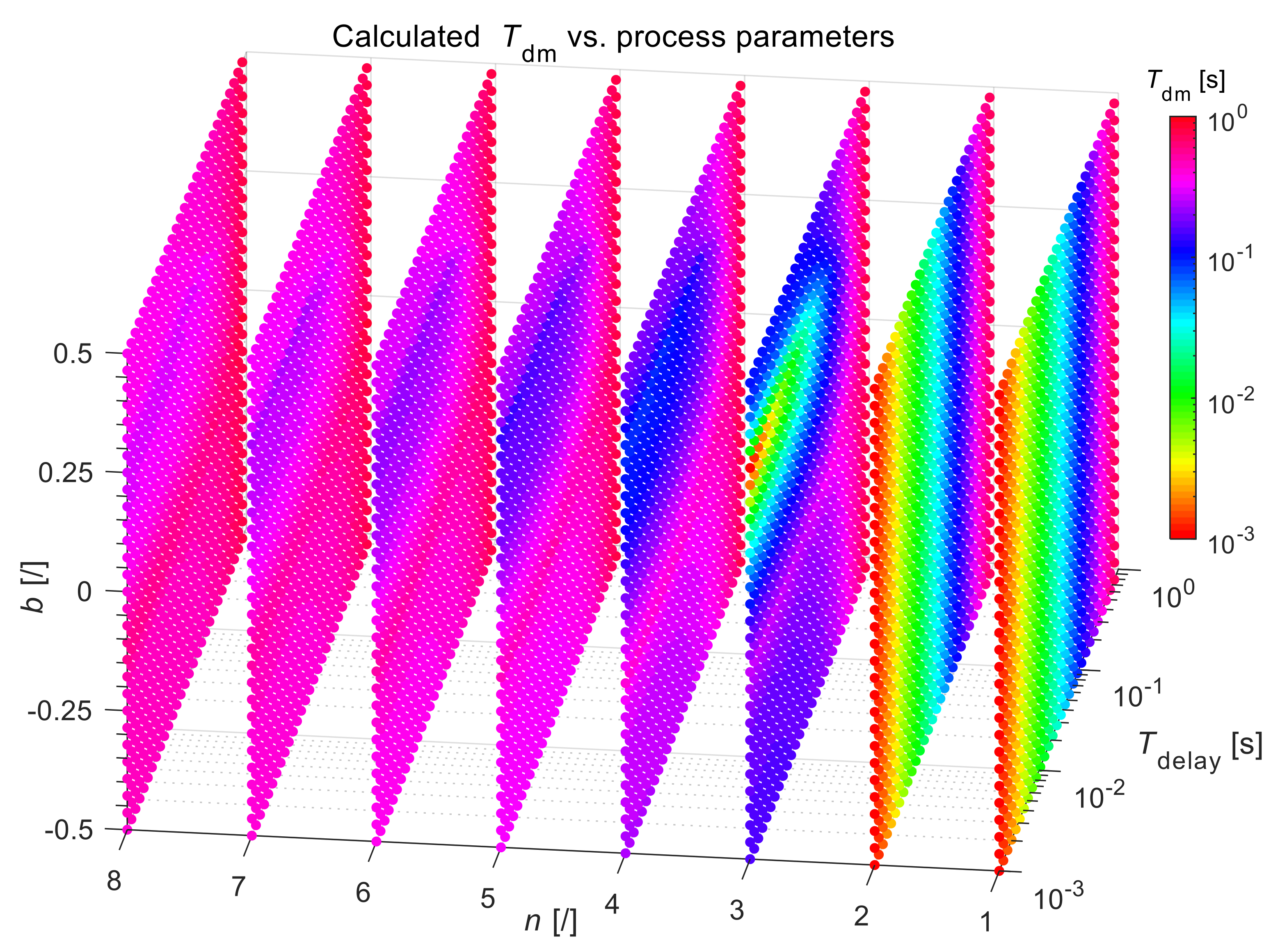
The calculated Process model (9) parameters b_1m and T_dm for the selected process G_P1 parameters are shown in Figure 3 and Figure 4, respectively. As can be seen from Figure 3 and Figure 4, the calculated process model parameters b_1m and T_dm for lower-order processes (n = 1, 2) are identical to the actual process parameters b and T_delay. For higher-order processes (n = 3–8), the calculated b_1m deviates from b, and becomes zero for a wider set of actual process parameters, while the calculated time delay T_dm becomes higher than the actual time delay T_delay, as expected.

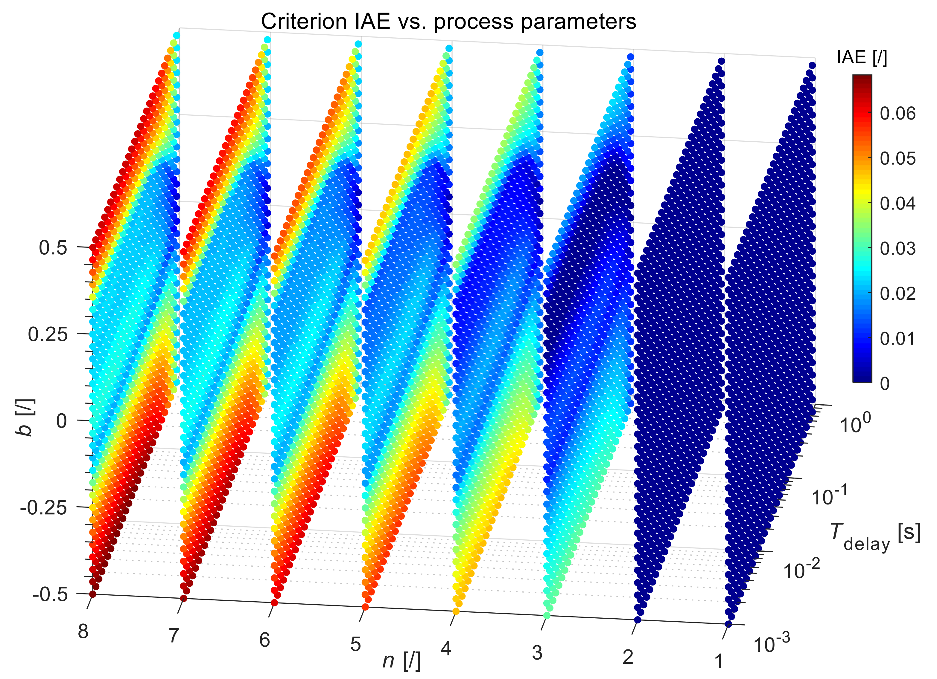
The IAE criterion values for the process G_P1 are shown in Figure 5. The IAE criterion is 0 for the first- and the second-order processes (perfect fit), and it increases as the process order and numerator time constant b increase. However, the maximum value of IAE remains relatively low (0.068).

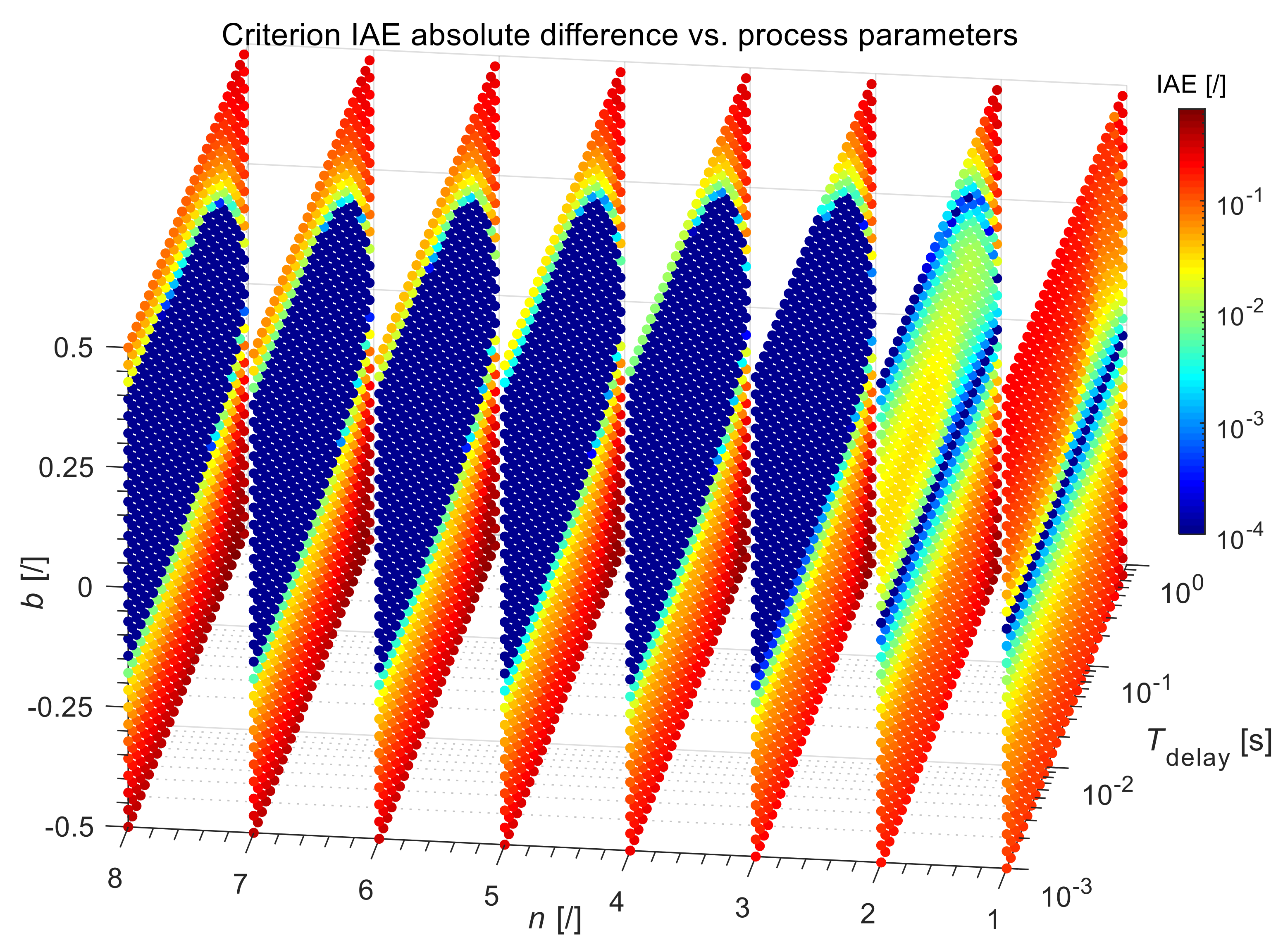
Next, the proposed model identification method was compared with that of Vrečko et al. [44] (the method with fixed b_1m = 0). For this purpose, the absolute difference of IAE criteria was calculated by the following expression:

$${\mathrm{IAE}}_{\Delta }={\mathrm{IAE}}_{\mathrm{Vrecko}}-{\mathrm{IAE}}_{\mathrm{proposed}}.$$

(26)

If the performance of both methods is identical, the calculated criterion difference will be 0, otherwise, the value will be larger.

The absolute difference of the IAE criterion for the process G_P1 is shown in Figure 6. As expected, the IAE values of both methods are identical in the cases where b_1m = 0. However, in other cases, the difference of IAE criteria confirms the superiority of the proposed model identification method. Note that the maximum difference of the IAE_Δ criterion is 0.67.

4.2. Model Identification from an Open-Loop Time Response of the Process

In this subsection, the proposed identification method was tested in the time-domain, i.e., the characteristic areas of the process are identified from an open-loop time response of a process during the steady-state change. For this purpose, the following common process models were selected:

$$\begin{gathered} G_{\mathrm{P}1}\left(s\right)=\frac{\left(1-0.2s\right)e^{-0.2s}}{\left(1+s\right)\left(1+0.2s\right)}, \\ {G}_{\mathrm{P}2}\left(s\right)=\frac{1}{{\left(1+0.25s\right)}^8}, \\ {G}_{\mathrm{P}3}\left(s\right)=\frac{0.5\left(1-0.5s\right)e^{-0.7s}}{\left(1+0.4s\right)\left(1+0.1s\right)\left(1+0.5s\right)}, \\ {G}_{\mathrm{P}4}\left(s\right)=\frac{2.15\left(1-2.7s\right)\left(1+6s+158.5s^2\right)e^{-14s}}{{\left(1+17.5s\right)}^4\left(1+20s\right)}, \\ {G}_{\mathrm{P}5}\left(s\right)=\frac{e^{-2s}}{\left(1+s\right)\left(1+10s\right)}, \\ {G}_{\mathrm{P}6}\left(s\right)=\frac{\left(1-s\right)e^{-s}}{{\left(1+s\right)}^5}., \\ {G}_{P7}\left(s\right)=\frac{\left(1-0.5s\right)e^{-s}}{{\left(1+s\right)}^2}. \end{gathered}$$

(27)

A step-change input signal was applied to the presented processes. Note that the sampling period was set to T_S = 1 ms. The output responses of the processes were then used to calculate the areas and consequently the parameters of the models.

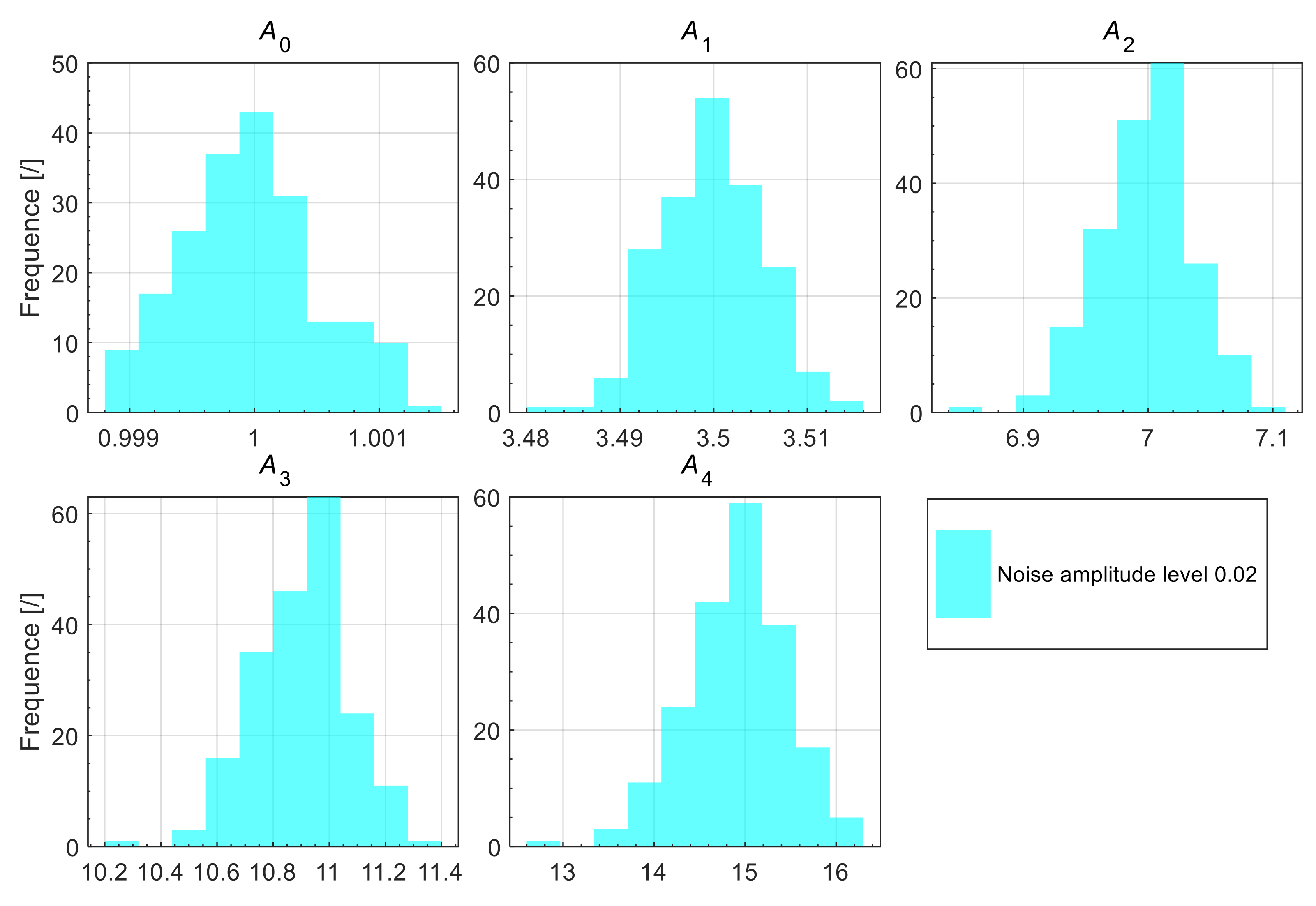
The calculated characteristic areas A₀–A₄ from the process responses are given in

Table 1. The calculated characteristic areas from the time responses of the process models.

	A0	A1	A2	A3	A4
GP1	1	1.6	1.78	1.82	1.83
GP2	1	2	2.25	1.875	1.289
GP3	0.5	1.1	1.252	1.0333	0.7114
GP4	2.15	216.51	12,942.13	594,451.35	23,117,961.95
GP5	1	13	135	1356.33	13,570.22
GP6	1	7	26.5	73.17	166.04
GP7	1	3.5	7	10.90	14.89

, according to the Expressions (4)–(6). Note that in order to reduce the numerical error, processes G_P1–G_P6 input and output signals were first filtered with a first-order low-pass filter with a time constant of 10 ms. Then, the parameters of Model (9) were calculated from the characteristic areas, according to the flowchart shown in Figure 1.

The processes G_P1–G_P3 were compared with three other model identification methods [28,33]. All the chosen methods provide analytical tuning formulas for calculating the model parameters. The first one was the method of Broida [33], which is intended for estimating the higher-order processes. The method provides the next model transfer function:

$$G_{\mathrm{M}}\left(s\right)=\frac{K_{\mathrm{M}}{e}^{-T_{\mathrm{dm}}s}}{{{\displaystyle \prod }}_{k=1}^n\left(1+\frac{a_{1\mathrm{m}}}{k}s\right)},$$

(28)

where n is the order of the model (1)–(6). The second was Åström’s method (time integral approach) [28], hereafter referred to as Åström (time integral). The method obtains the next second-order model:

$$G_{\mathrm{M}}\left(s\right)=\frac{K_{\mathrm{M}}{e}^{-T_{\mathrm{dm}}s}}{1+a_{1\mathrm{m}}s+a_{2\mathrm{m}}{s}^2}.$$

(29)

The third was Åström’s method (model-fitting approach) [28], hereafter referred to as Åström (model-fitting). The method obtains the next first-order model:

$$G_{\mathrm{M}}\left(s\right)=\frac{K_{\mathrm{M}}{e}^{-T_{\mathrm{dm}}s}}{1+a_{1\mathrm{m}}s}.$$

(30)

The identified model parameters (28)–(30) were calculated from the step responses of the processes.

Processes G_P4–G_P6 are compared with other step and relay identification methods that will be described individually. The model parameters for these methods were taken from the literature.

The sensitivity to the process noise was tested on the process G_P7.

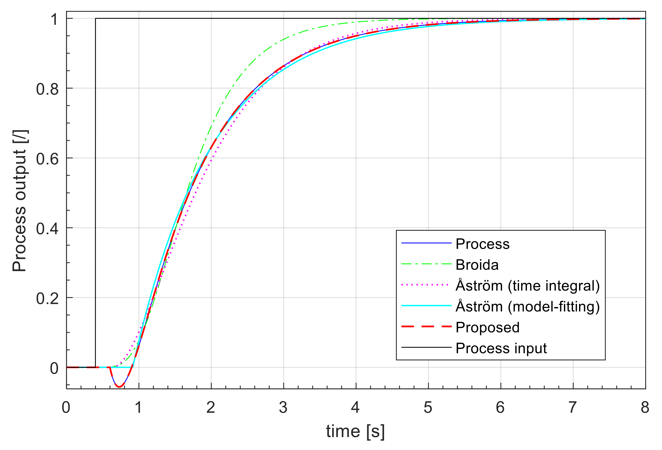
Case 1

The Broida, two Åströms methods, and the proposed method were tested on the second-order process with zero plus time delay. The estimated model parameters process G_P1 are given in

Table 2. The estimated model parameters for the process G_P1.

	KM	a1m	a2m	Tdm	b1m	n
Broida [33]	1	0.5679	/	0	/	6
Åström (time integral) [28]	1	1.3661	0.46657	0.2338	/	/
Åström (model-fitting) [28]	1	1.0857	/	0.5142	/	/
Proposed	1	1.2	0.2	0.2	–0.2	/

.

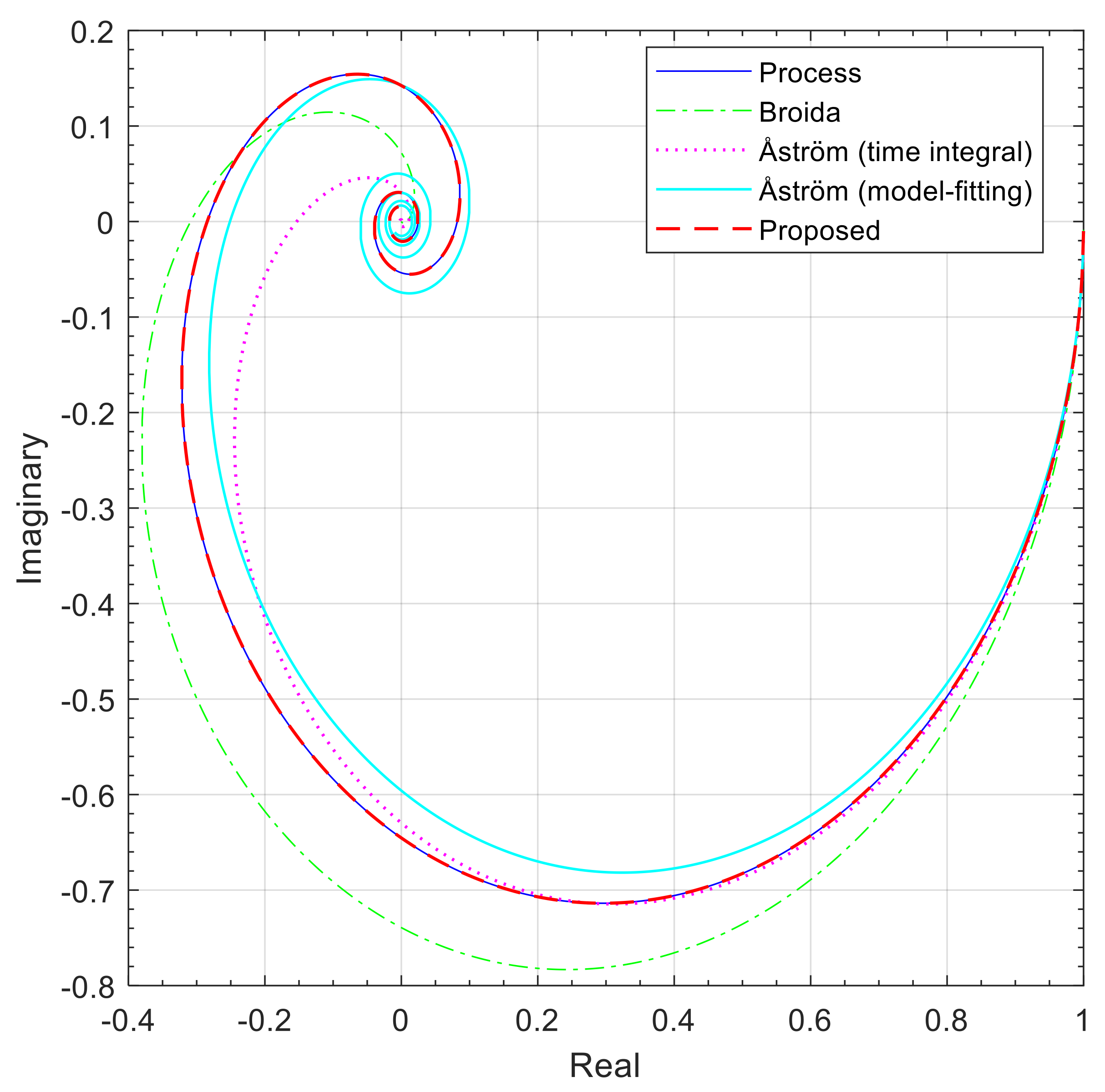
Figure 7, Figure 8 and Figure 9 compare the step responses for u = 1, Bode, and Nyquist plots of the aforementioned identification methods. The criteria values are given in

Table 3. The criteria values for the process G_P1.

	IAE	ERR
Broida [33]	0.208	0.0446
Åström (time integral) [28]	0.085	0.0213
Åström (model-fitting) [28]	0.0565	0.0139
Proposed	6.813 × 10–5	1.884 × 10–5

. Note that for the calculation of the criterion ERR, ω₀ = 6.25 × 10^–3 and ω_C = 3.369 rad/s. The Nyquist plot in all the examples is plotted in the frequency range from ω₀ to ω₀ × 10⁴ rad/s. Similarly, the Bode graph in all the examples is plotted in the frequency range from ω₀ × 10 to ω_C rad/s.

The figures show that the proposed identification method gives a perfect fit between the identified and the actual process model. This is confirmed by the lowest criteria in the time- and the frequency-domain. The Åström (model-fitting) method was ranked second.

Case 2

The Broida, two Åströms methods, and the proposed method were tested on the higher-order process. The estimated model parameters for the process G_P2 are given in

Table 4. The estimated model parameters for the process G_P2.

	KM	a1m	a2m	Tdm	b1m	n
Broida [33]	1	0.6736	/	0.4259	/	6
Åström (time integral) [28]	1	1.0313	0.26589	0.9687	/	/
Åström (model-fitting) [28]	1	0.92323	/	1.0767	/	/
Proposed	1	1.1309	0.3895	0.8690	0	/

.

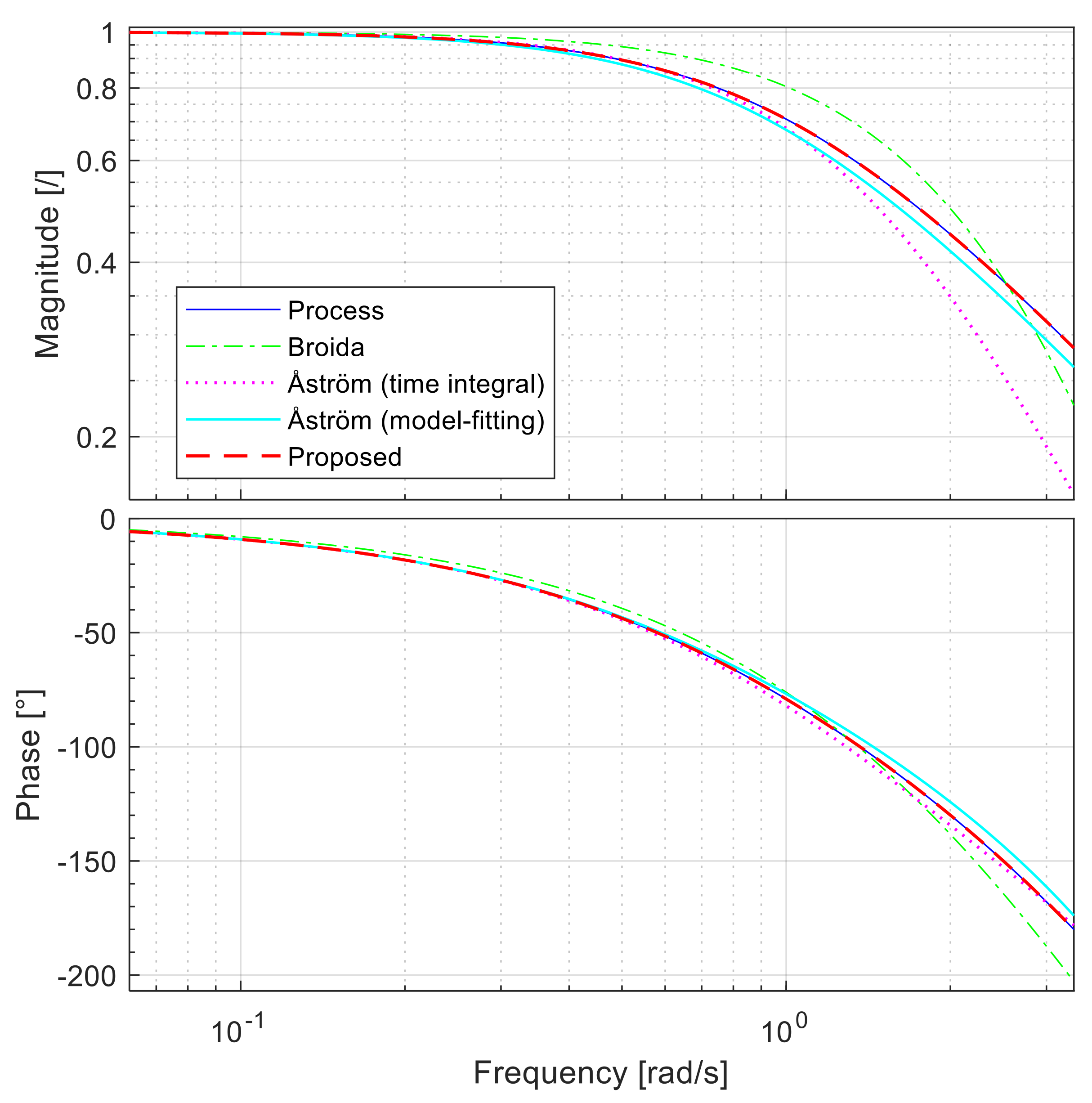
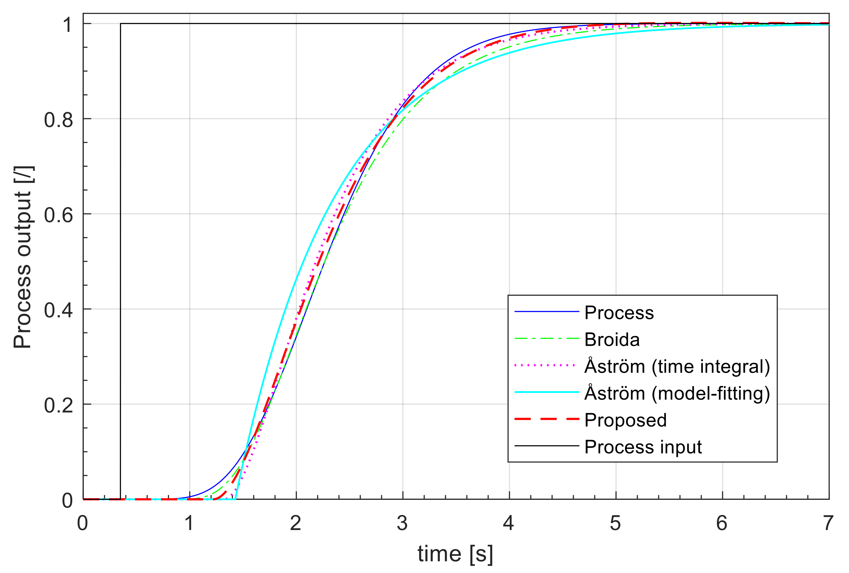
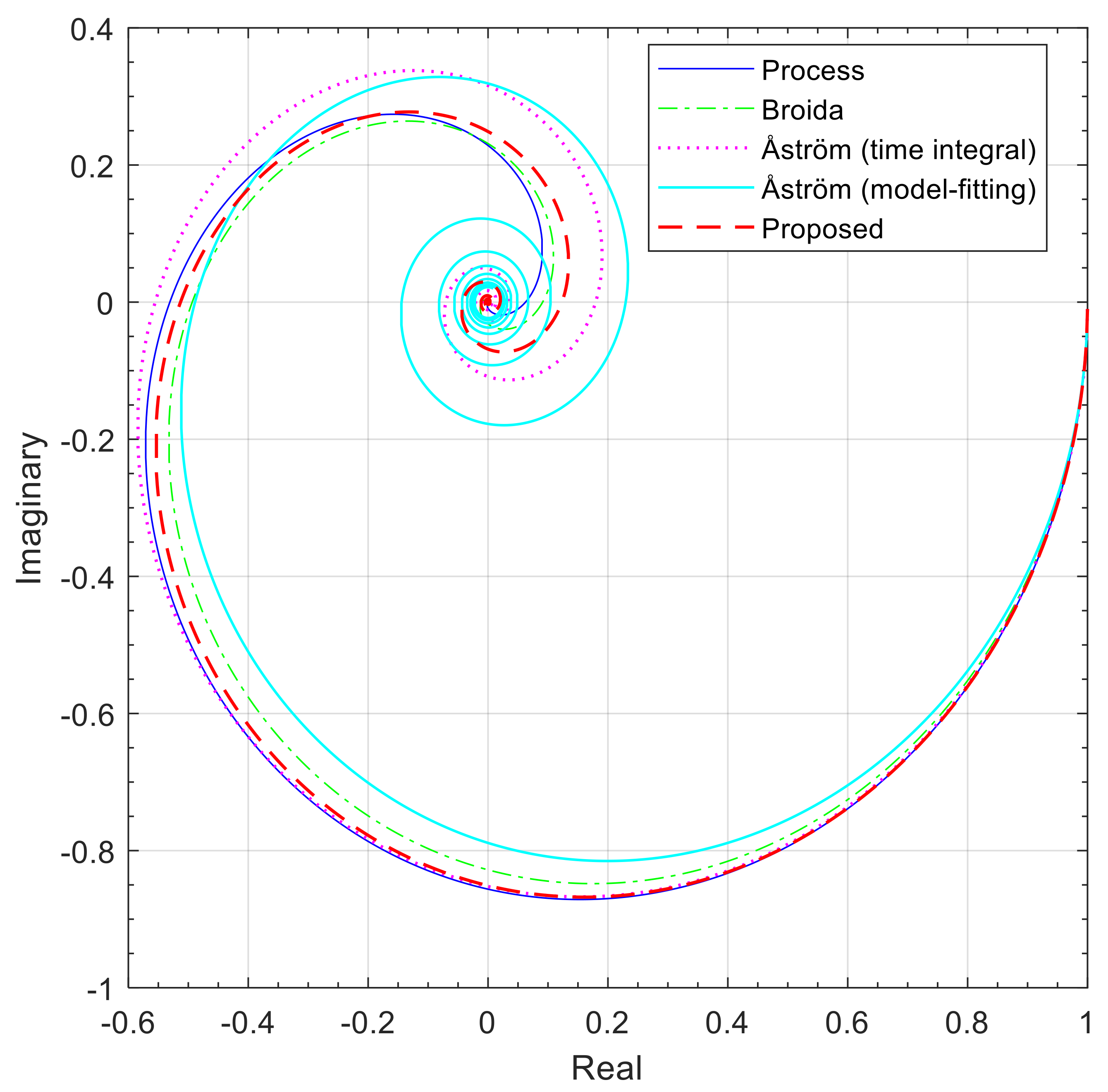
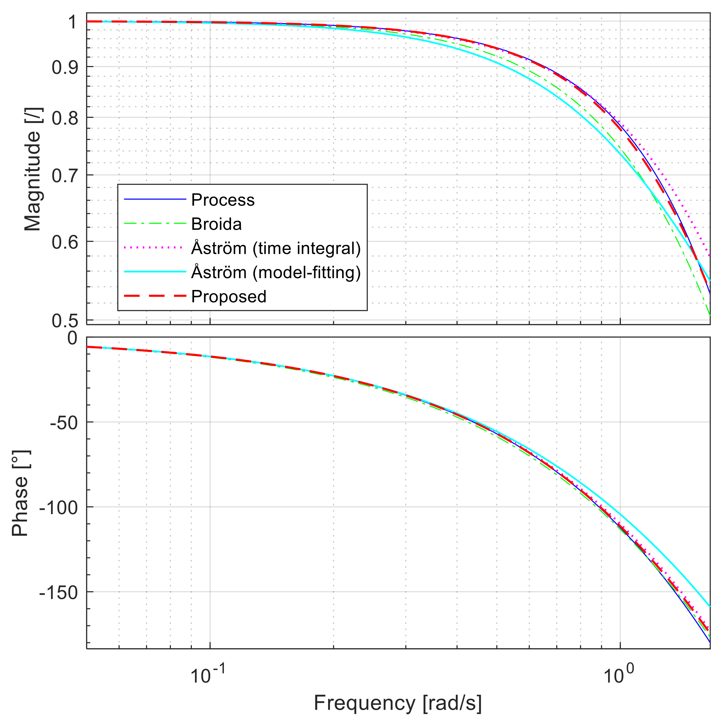
Figure 10, Figure 11 and Figure 12 compare the step responses for u = 1, Bode, and Nyquist plots on the aforementioned identification methods. The criteria values are given in

Table 5. The criteria values for the process G_P2.

	IAE	ERR
Broida [33]	0.0781	0.0143
Åström (time integral) [28]	0.0814	7 × 10–3
Åström (model-fitting) [28]	0.199	0.0258
Proposed	0.0537	3.22 × 10–3

. Note that for the calculation of the criterion ERR, ω₀ = 5 × 10^–3 and ω_C = 1.6569 rad/s.

The figures show that the proposed identification method gives an excellent approximation of the process at low frequencies. At higher frequencies, some smaller deviation can be observed. Nevertheless, the proposed method achieves the lowest criteria values in the time- and frequency-domain. The second was Åström (time integral) in the frequency-domain and Broida method in the time-domain.

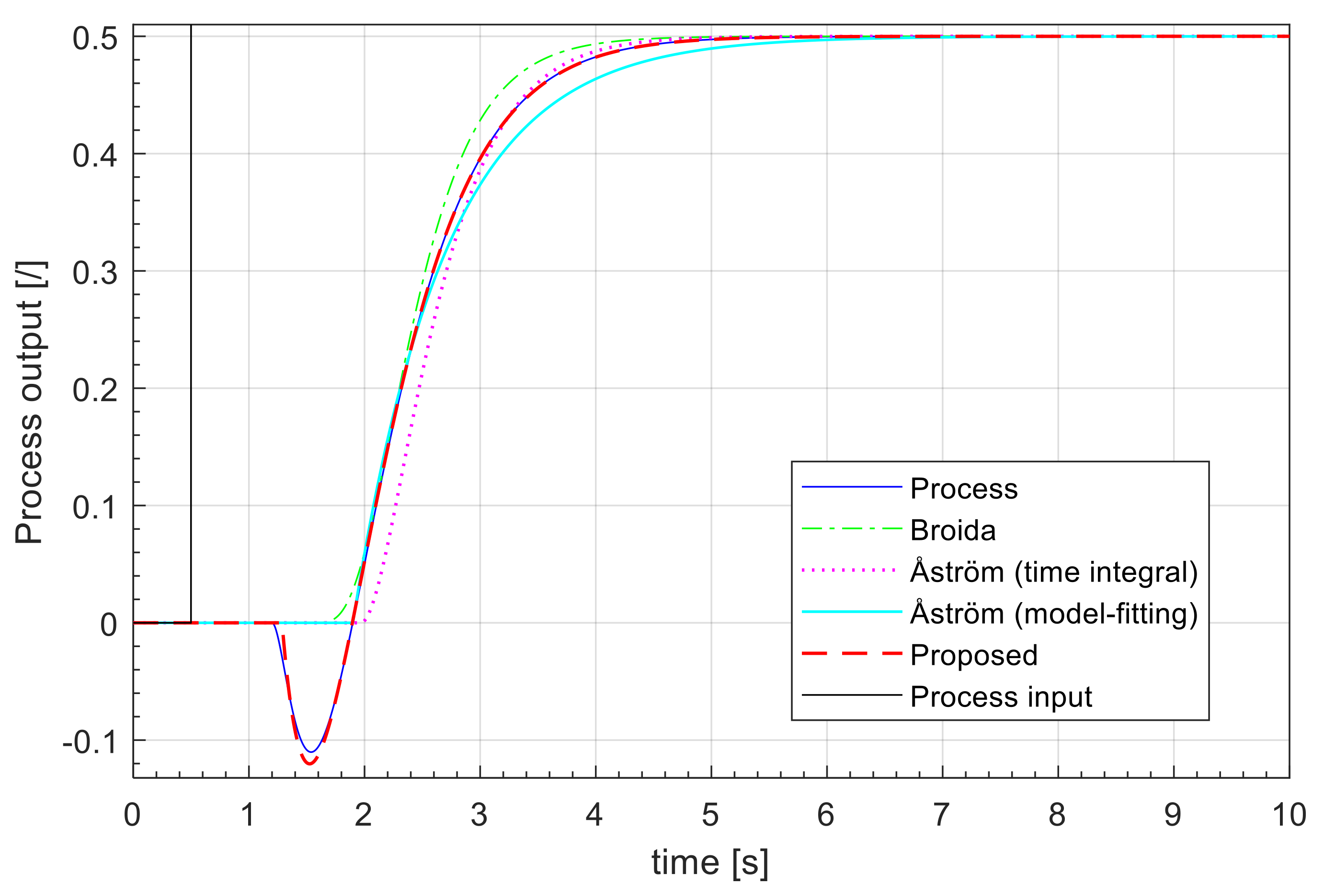
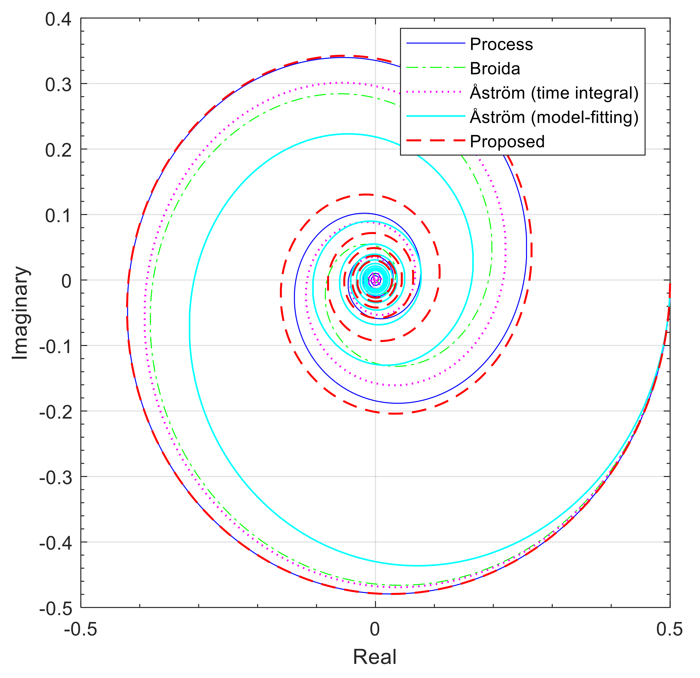
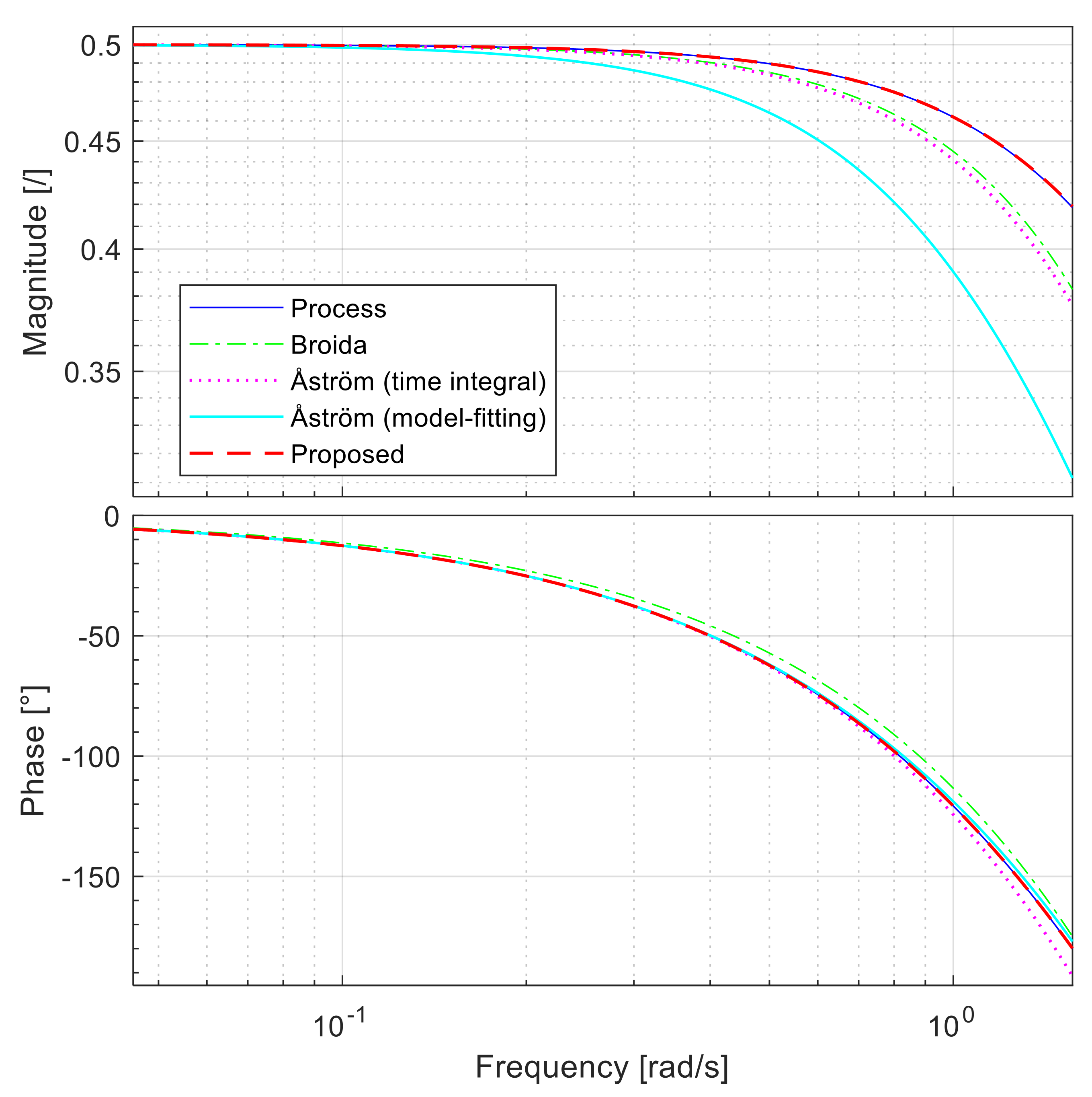
Case 3

The Broida method, two Åströms methods, and the proposed method were tested on a third-order process with zero plus time delay. This process was described in [47,48,49]. The estimated model parameters for the process G_P3 are given in

Table 6. The estimated model parameters for the process G_P3.

	KM	a1m	a2m	Tdm	b1m	n
Broida [33]	0.5	0.4067	/	1.0067	/	6
Åström (time integral) [28]	0.5	0.73243	0.13411	1.4675	/	/
Åström (model-fitting) [28]	0.5	0.8012	/	1.3988	/	/
Proposed	0.5	0.9149	0.2093	0.7867	–0.4984	/

.

Figure 13, Figure 14 and Figure 15 compare the step responses for u = 1, Bode, and Nyquist plots on the aforementioned identification methods. The criteria values are given in

Table 7. The criteria values for the process G_P3.

	IAE	ERR
Broida [33]	0.161	0.0188
Åström (time integral) [28]	0.176	7.21 × 10–3
Åström (model-fitting) [28]	0.165	0.015
Proposed	0.0103	4.36 × 10–5

. Note that for the calculation of the criterion ERR, ω₀ = 4.55 × 10^–3 and ω_C = 1.567 rad/s.

The figures show that the model, obtained by the proposed identification method, provides an excellent approximation of the process in a wide frequency range. At very high frequencies (Nyquist plot), some deviation can be seen. From Figure 13, it can be seen that the proposed method also provides a good approximation in the time-domain. This is confirmed by the lowest criteria in the time- and the frequency-domain. The Åström method (time integral) was ranked second in the frequency-domain, and the Broida method was ranked second in the time-domain.

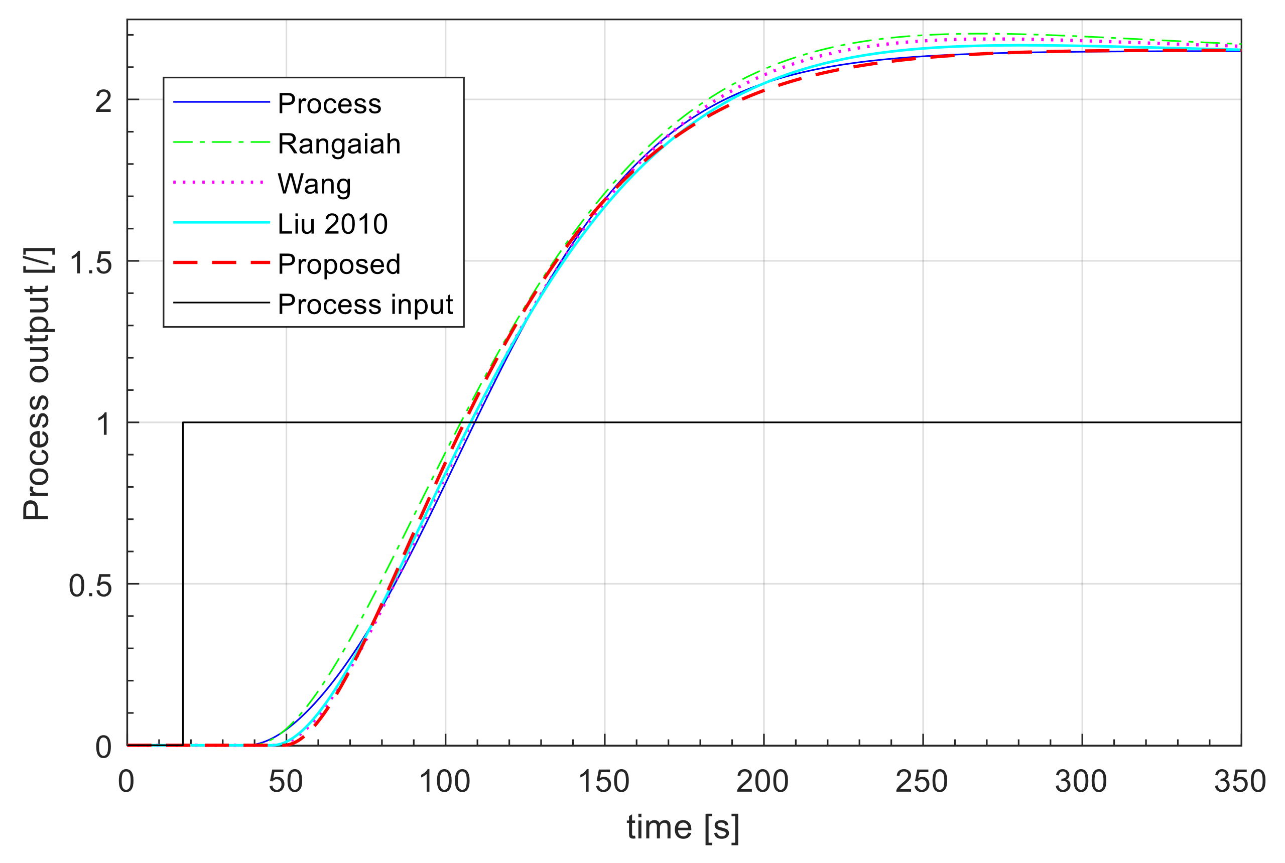
Case 4

The process G_P4 (higher-order process with a higher-order numerator and time delay) was compared with the three-step identification methods [25,31,50]. The first one is the method of Rangaiah and Krishnaswamy [31], hereafter referred to as Rangaiah. The method for estimating the model uses three-point fitting. The estimated model parameters for process G_P4 in this method are published in [7]. The second method is the method of Wang and Zhang [50], hereafter referred to as Wang. The method for estimating the model uses a time integral approach. The third method is the method of Liu and Gao [25], hereafter referred to as Liu 2010. The method for estimating the model uses a frequency response fitting. All the methods presented provide the second-order model with time delay (8). The estimated model parameters for all presented and proposed methods for process G_P4 are given in

Table 8. The estimated model parameters for the process G_P4.

	KM	a1m	a2m	Tdm	b1m
Rangaiah [31]	2.15	71.99	2234.7	21.56	/
Wang [50]	2.15	69.63	1939.4	28.58	/
Liu 2010 [25]	2.14	70.98	1903.1	27.96	/
Proposed	2.15	69.04	1433.8	31.66	0

.

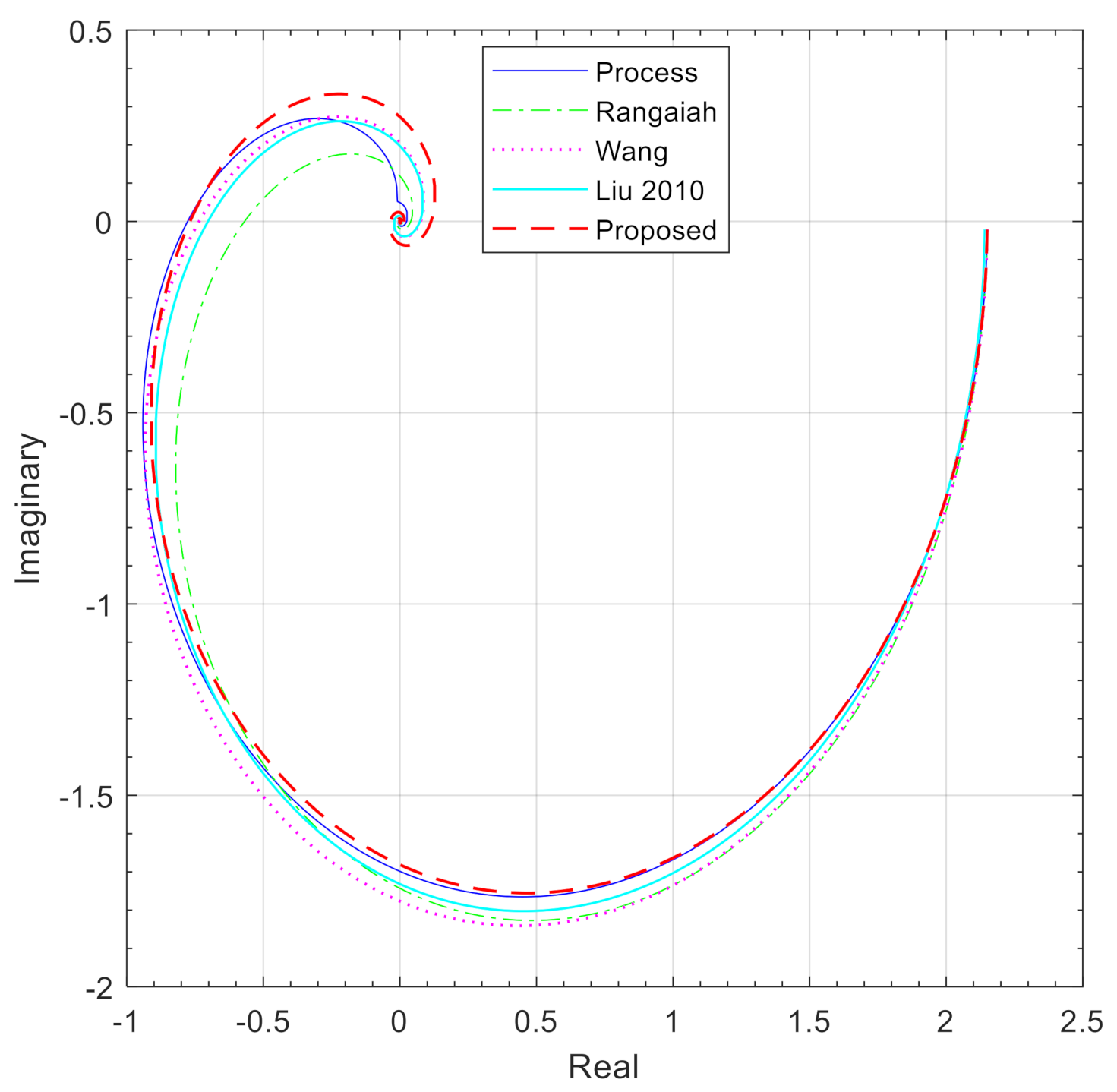
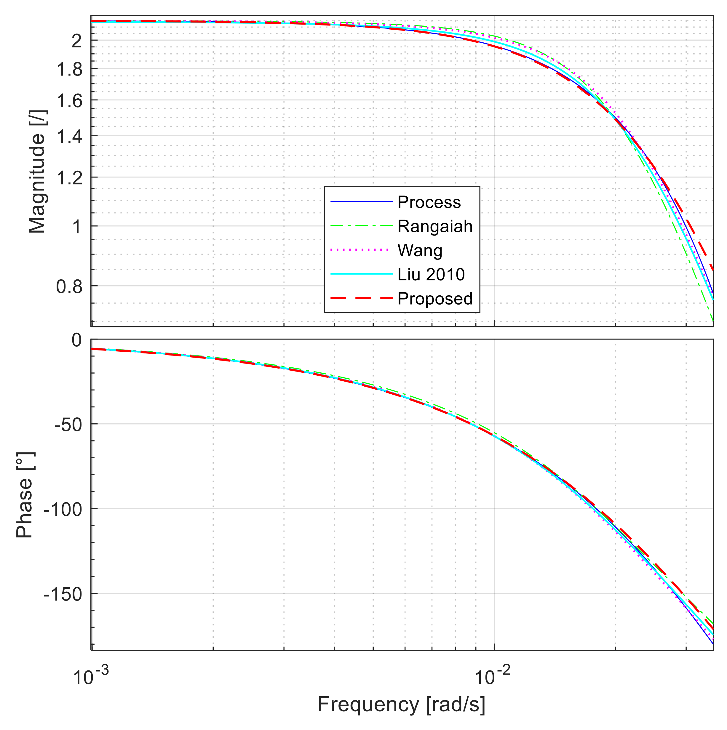
Figure 16, Figure 17 and Figure 18 compare the step responses for u = 1, Bode, and Nyquist plots between the aforementioned identification methods. The criteria values are given in

Table 9. The criteria values for the process G_P4.

	IAE	ERR
Rangaiah [31]	7.304	0.0401
Wang [50]	3.971	0.0233
Liu 2010 [25]	5.250	0.0185
Proposed	2.968	0.0111

. For the calculation of the criterion ERR, ω₀ = 9.931 × 10^–5 and ω_C = 3.505 × 10^–2 rad/s.

The figures show that the proposed identification method gives an excellent approximation of the process at low frequencies, while some deviations can be seen at higher frequencies. Nevertheless, the proposed method obtained the lowest criterion values in the time- and frequency-domain. The Liu 2010 method was ranked second in the frequency-domain, and the Wang method was ranked second in the time-domain.

Case 5

The process G_P5 (second-order process with time delay) was compared with the three relay identification methods [51,52,53]. The first is the describing function approach of Li et al. [51], hereafter referred to as Li. The second is the method of Liu et al. [52], hereafter referred to as Liu 2008. The Liu method for estimating the model uses a curve-fitting approach. The third is the method of Ramakrishnan and Chidambaram [53], hereafter referred to as Ramakrishnan. The method for estimating the model uses frequency response fitting. All the methods presented provide the second-order model with time delay (8). The estimated model parameters for all presented and proposed methods for process G_P5 are given in

Table 10. The estimated model parameters for the process G_P5.

	KM	a1m	a2m	Tdm	b1m
Li [51]	0.853	8.566	8.528	2	/
Liu 2008 [52]	1	11.00	10.07	1.999	/
Ramakrishnan [53]	1.05	11.04	12.41	1.814	/
Proposed	1	11.00	10.03	2.071	0.0743

.

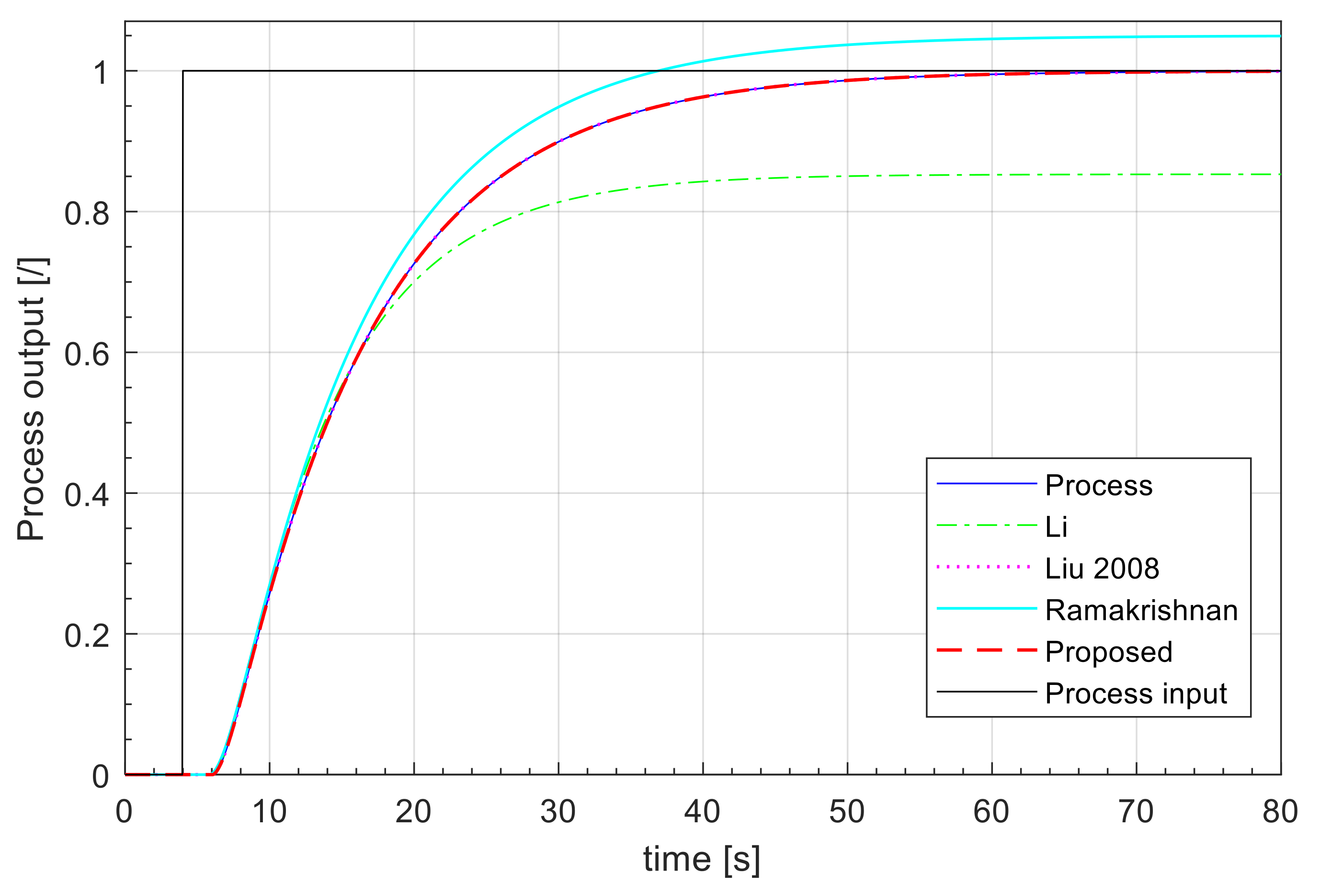
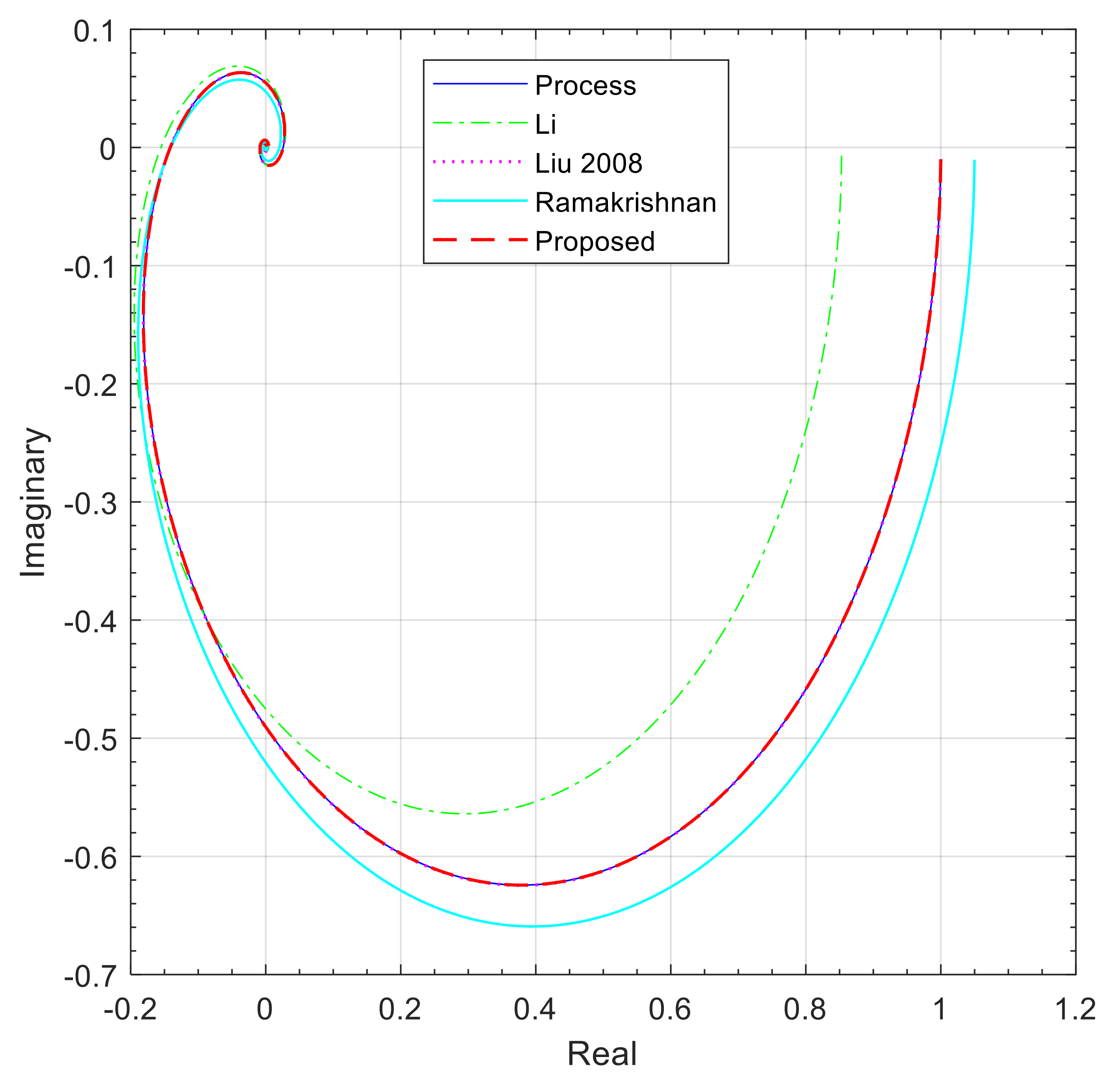
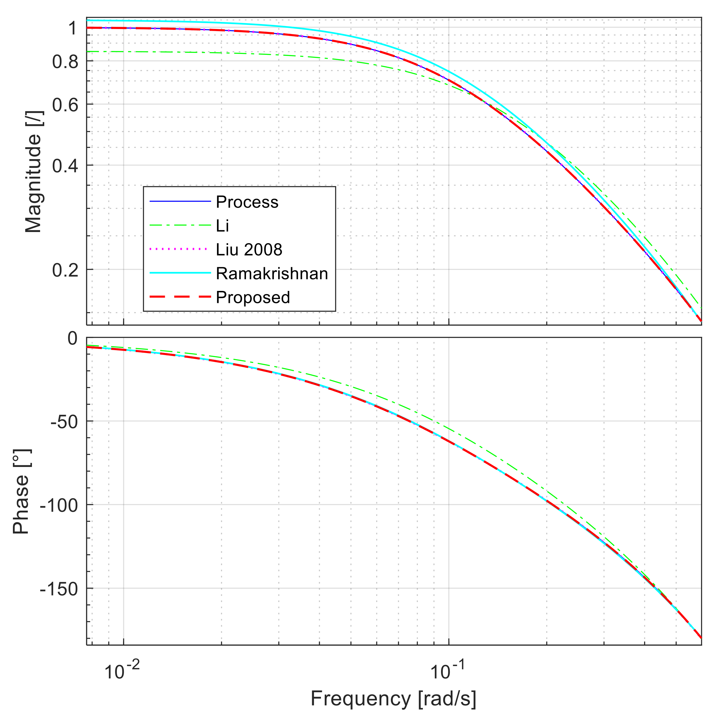
Figure 19, Figure 20 and Figure 21 compare the step responses for u = 1, Bode, and Nyquist plots between the aforementioned identification methods. The criteria values are given in

Table 11. The criteria values for the process G_P5.

	IAE	ERR
Li [51]	30.86	0.1148
Liu 2008 [52]	4.806 × 10–3	1.451 × 10–4
Ramakrishnan [53]	11.31	0.04147
Proposed	2.237 × 10–4	7.284 × 10–6

. The criterion ERR is calculated in the frequency region from ω₀ = 7.692 × 10^–4 to ω_C = 0.599 rad/s.

The figures again show that the proposed identification method gives an excellent approximation of the process in the whole frequency range. This is confirmed by the lowest criteria in the time- and the frequency-domain. The Liu 2008 method was ranked second.

Case 6

The process G_P6 (higher-order non-minimum phase process with time delay) was compared with the three relay identification methods [18,22,54]. The first one is the describing function approach of Shen et al. [22], hereafter referred to as Shen. The estimated model parameters for process G_P6 for this method are published in [7]. The second is the method of Kaya and Atherton [18], hereafter referred to as Kaya. The method for estimating the model uses a curve-fitting approach. The third is the method of Liu and Gao [54], hereafter referred to as Liu 2009. The method for model estimation uses a frequency response fitting. All the methods presented provide the second-order model with time delay (8). The estimated model parameters for all the methods for process G_P6 are given in

Table 12. The estimated model parameters for the process G_P6.

	KM	a1m	a2m	Tdm	b1m
Shen [22]	1	2.96	2.1904	4.56	/
Kaya [18]	1	2.9534	2.1806	4.125	/
Liu 2009 [54]	0.9992	2.9562	2.1848	4.037	/
Proposed	1	3.2307	2.9101	2.9836	–0.7856

.

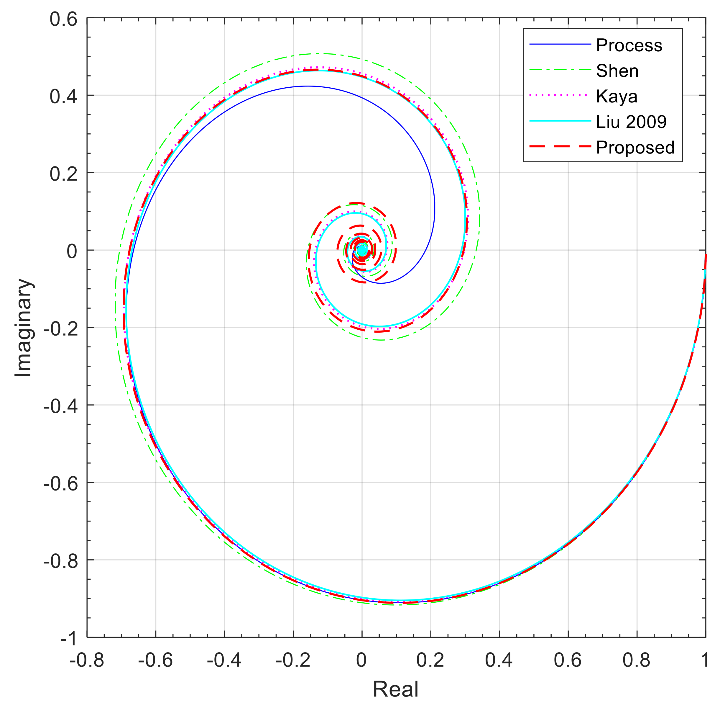
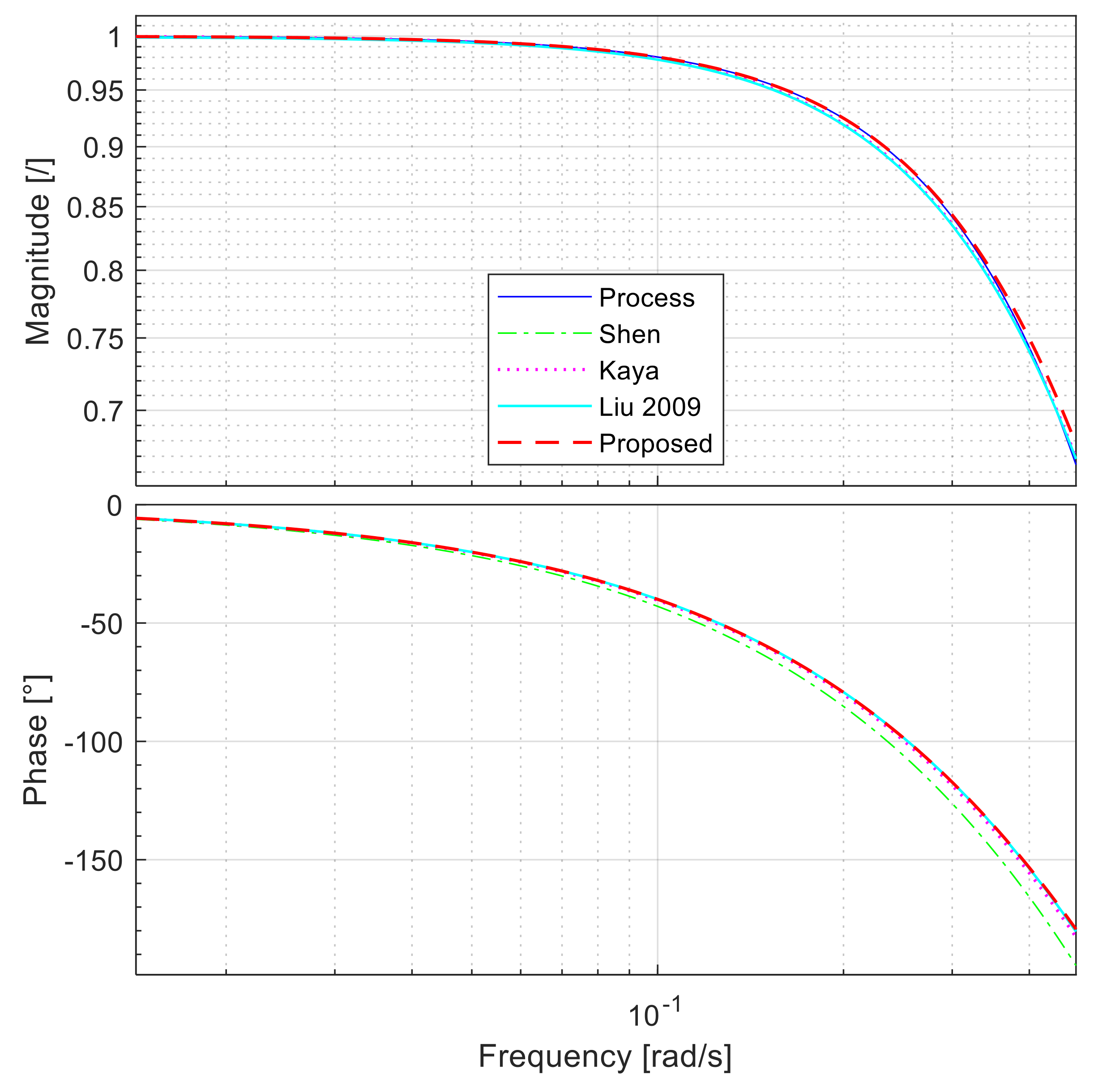
Figure 22, Figure 23 and Figure 24 compare the step responses for u = 1, Bode, and Nyquist plots between the aforementioned identification methods. The criteria values are given in

Table 13. The criteria values for the process G_P6.

	IAE	ERR
Shen [22]	0.6	0.037
Kaya [18]	0.178	5.78 × 10–3
Liu 2009 [54]	0.193	2.07 × 10–3
Proposed	0.149	6.713 × 10–4

. The criterion ERR is calculated in the frequency region between ω₀ = 1.429 × 10^–3 and ω_C = 0.476 rad/s.

The figures show that the proposed identification method gives an excellent approximation of the process at low frequencies. At higher frequencies, some deviation can be seen. Nevertheless, the proposed method obtained the lowest criterion values in the time- and frequency-domain. The Liu 2009 method was ranked second in the frequency-domain, and the Kaya method was ranked second in the time-domain.

Case 7

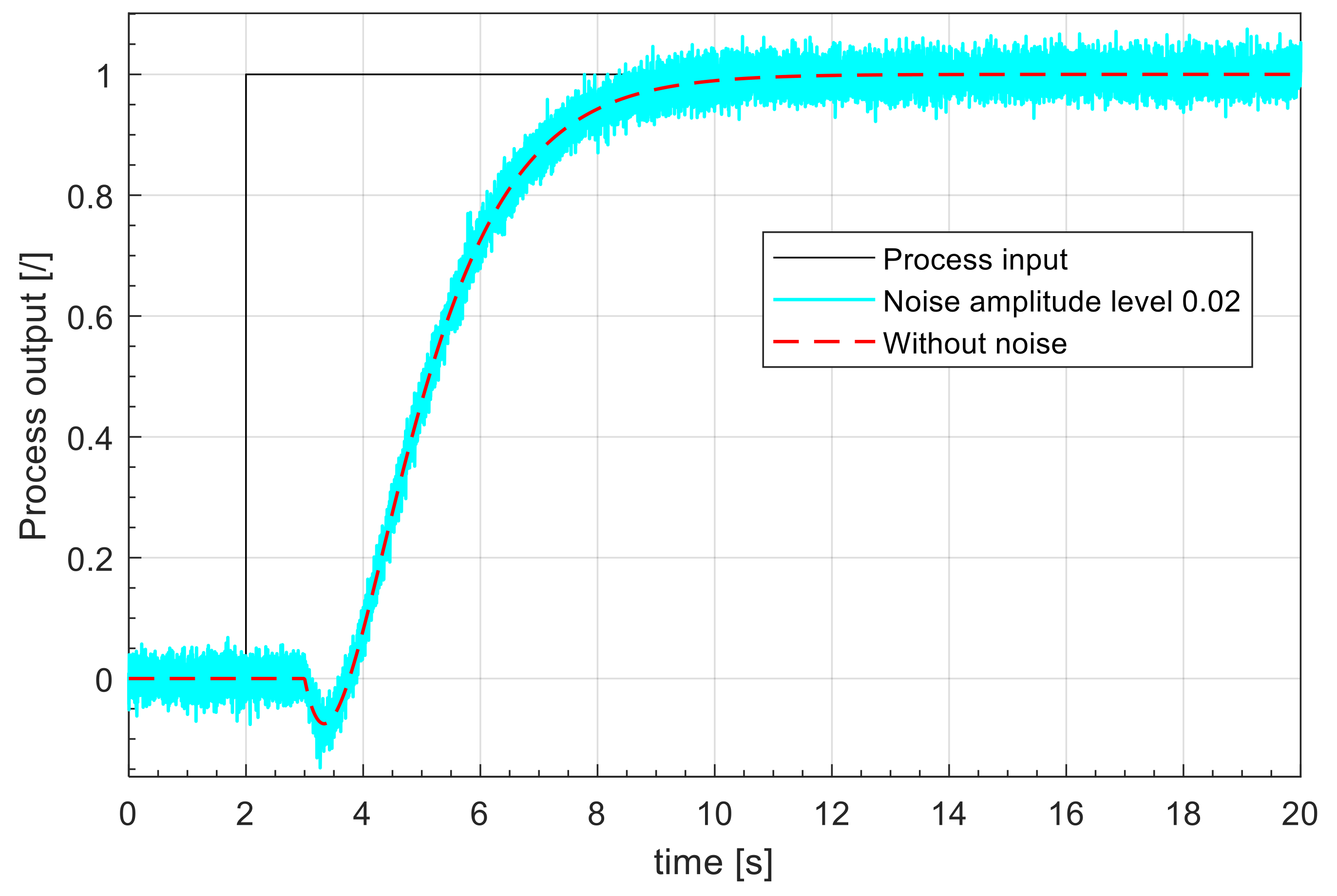
The process G_P7 is the second-order non-minimum phase process with time delay. Here, the sensitivity to the process noise was tested, rather than comparison to other methods.

The test was performed as follows. First, we obtained 200 step responses of the process, where a random white noise signal with power 1 multiplied by gain 2 × 10⁻² was added as measurement noise to the process output. The typical step response of the process with noise is shown in Figure 25. The initial steady-state of the process was calculated by averaging the process signals between t = 0 s and t = 2 s, whereas the final steady-state was obtained from the average signal in the interval between t = 17 s and t = 20 s. Multiple integrations of the process input and output signals were performed between t = 2 s and t = 15 s.

Note that to reduce numerical error, the process input and output signals for all 200 responses were filtered using a second-order filter, defined by the next transfer function before multiple integrations were performed:

$$G_{\mathrm{LP}2}=\frac{1}{{\left(1+0.05s\right)}^2}.$$

(31)

Then, characteristic areas were calculated for all responses. The histograms of the calculated areas are shown in Figure 26.

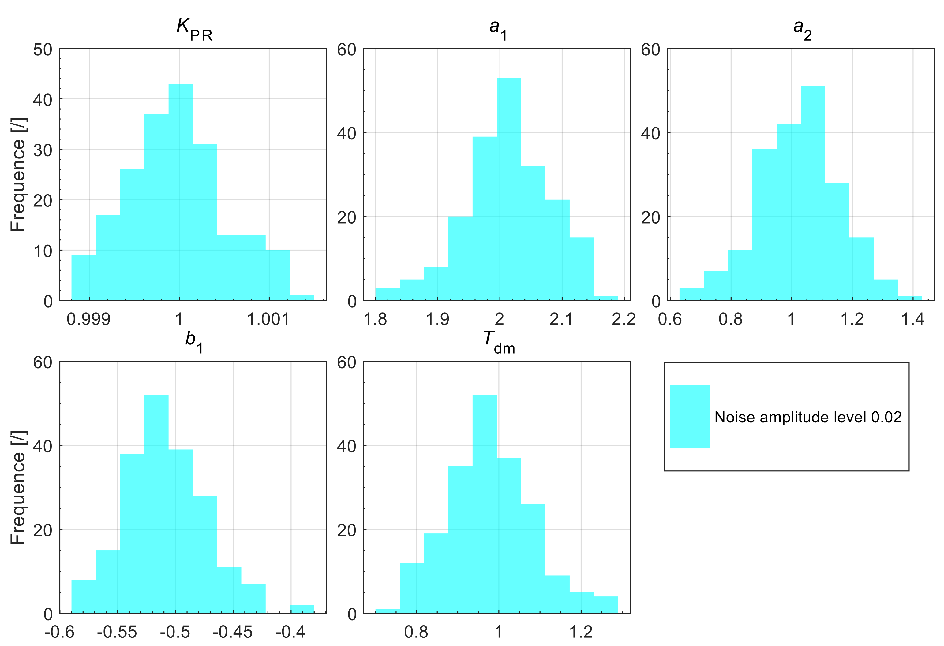
As can be seen, the dispersion of the calculated areas is not that significant, even with a relatively high noise amplification. The obtained surfaces were then used to calculate the process model parameters. The histograms of the parameters are shown in Figure 27.

As can be seen from Figure 27, the dispersion of the process parameters is not large.

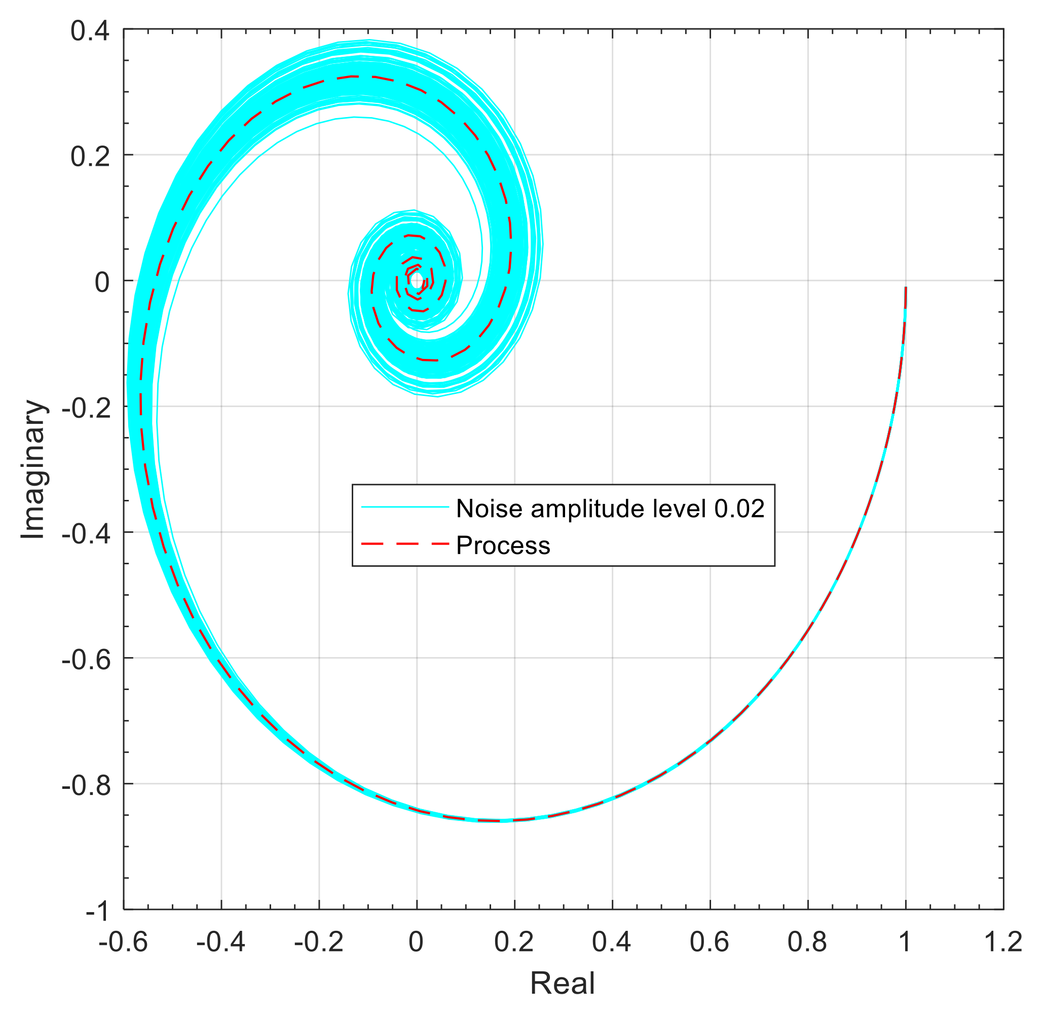
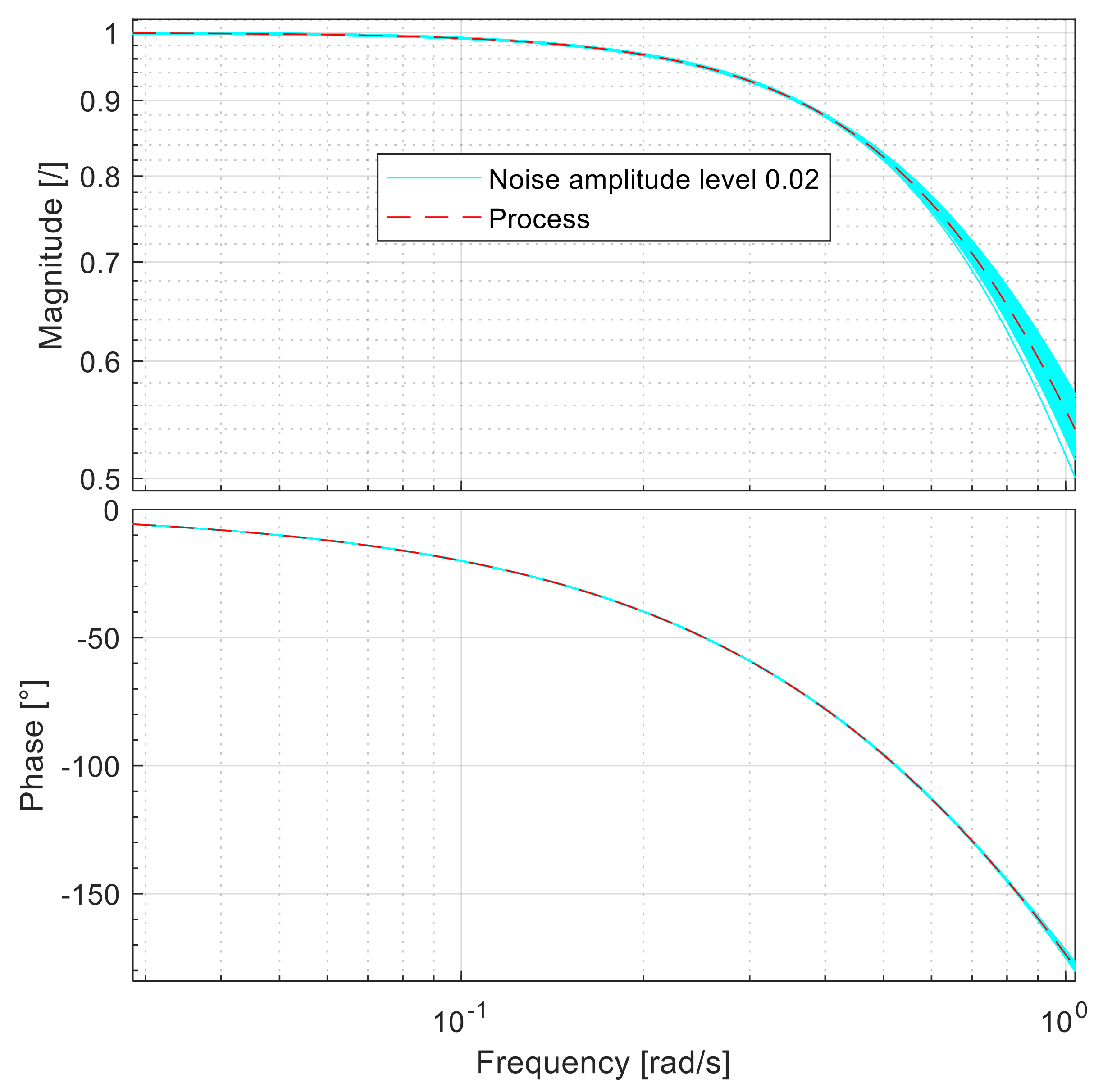
The quality of the obtained models is shown in Figure 28 and Figure 29. Figure 28 shows the Nyquist plot for the computed process models compared to the original process (dashed red line). It can be seen that the calculated process models are very close to the actual process model, especially at lower frequencies. A similar conclusion can be drawn from the Bode plot (Figure 29), where it can be seen that the calculated process models are very close to the actual process model.

The results indicate that the proposed method can be used, even in the presence of moderate process noise.

5. Conclusions

In this paper, an analytical method is proposed to identify the five-parameter model (second-order process with zero plus time delay) directly from the characteristic areas, i.e., from the closed-loop or open-loop time responses of the process (in the time-domain), or from the general-order transfer function with time delay (in the frequency-domain). The only parameter that is required by the user is the type of process (minimum phase or non-minimum phase process), which in practice can be easily determined from the time response of the process.

The method can also be used to reduce the HO process model, to obtain the process model from the original process of infinite order (e.g., heat transfer processes), or to obtain the process model containing the sum of the different process delays. Moreover, the method can also be used to obtain integrating process models [41,42].

The proposed identification method was tested on several illustrative examples and compared with other identification methods. Both the model identification from a general-order transfer function with a time delay (in the frequency-domain) and from the time response of an open-loop process (in the time-domain) were tested. The obtained models were evaluated according to the criteria IAE (time response error), and ERR (frequency response error). The comparison with existing methods showed the superiority of the proposed method. In addition, the efficiency of the identification algorithm was tested on higher-order processes with zero and time delay. The test confirmed that the algorithm works properly for a wide family of process models, even in the presence of moderate process noise.

Future work will include more intensive testing of the proposed method under process noise.