A Mathematical Program for Scheduling Preventive Maintenance of Cogeneration Plants with Production

Abstract

This paper considers the scheduling of preventive maintenance for the boilers, turbines, and distillers of power plants that produce electricity and desalinated water. It models the problem as a mathematical program (MP) that maximizes the sum of the minimal ratios of production to the demand of electricity and water during a planning time horizon. This objective encourages the plants’ production and enhances the chances of meeting consumers’ needs. It reduces the chance of power cuts and water shortages that may be caused by emergency disruptions of equipment on the network. To assess its performance and effectiveness, we test the MP on a real system consisting of 32 units and generate a preventive maintenance schedule for a time horizon of 52 weeks (one year). The generated schedule outperforms the schedule established by experts of the water plant; it induces, respectively, 16% and 12% increases in the surpluses while either matching or surpassing the total production. The sensitivity analysis further indicates that the generated schedule can handle unforeseen longer maintenance periods as well as a 120% increase in demand—a sizable realization in a country that heavily relies on electricity to acclimate to the harsh weather conditions. In addition, it suggests the robustness of the schedules with respect to increased demand. In summary, the MP model yields optimal systematic sustainable schedules.

1. Introduction

Preventive maintenance (PM) is crucial to many service and manufacturing industries. Their routine application avoids unexpected equipment breakdown that, otherwise, would not only negatively impact the reliability of the logistic chain, but would also cause sizable losses, reduced productivity, and deteriorated quality of products and services. Many companies (from different industrial sectors) resort to scheduling PMs with the objective of optimizing service delivery, be it in terms of continuity or quality. For example, in the transport sector, ships [1,2], trains [3,4], and airplanes [5] are subject to different types of PMs, with some of them being daily, monthly, or usage-dependent. In manufacturing, some environments resort to maintenance events to allow for machine cooling [6] or to avoid slowing down the processing times [7]. Similarly, some plants resort to PMs to minimize the disruption of their supply [8].

1.1. Motivation

In power plants, PMs prevent failures, which could cause a general blackout not only of the areas served by the power plant, but of the complete electric grid. In harsh weather conditions, such as in the 2021 Texas case [9], a blackout translates into depriving households, industrial factories, and businesses not only of electricity, but also of heating and air conditioning, causing a chain reaction that makes it impossible for populations to access basic necessities. It affects the most deprived, causing many deaths and extreme medical emergencies. Restoring the grid is not instantaneous. It generally takes a couple of hours but may extend to several days depending on the severity of the equipment failure. Examples of such power plants are cogeneration energy plants that produce both electricity and water.

In arid/hot countries, the production of electricity and desalination of sea water are of prime importance. Drinking water is a scarce resource, while harsh weather conditions make the consumption of electricity for air conditioning purposes a necessity for any sustainable form of life. Cogeneration energy plants produce fresh water and electricity in more than 120 countries [10]. They owe their worldwide spread to their efficiency, reliability and economic value. To remain reliable over time, these plants require periodic PMs, according to a predefined preventive maintenance schedule (PMS).

1.2. Problem Statement and Contribution

A PMS is a set of repetitive actions undertaken for the maintenance of an equipment with the objective of its examination and renewal. For cogeneration plants, it is particularly crucial to the reliability of the power generation system: it discovers and eliminates a large number of unexpected failures that, in turn, cause a domino effect. It must be coordinated with the production. Subsequently, optimizing a PMS consists of finding the “best”sequence of maintenance activities for each unit of a plant in each period of a planning horizon such that this sequence minimizes water and power outages, subject to technical and demand functional requirements. This problem is particularly complex for two reasons. First, a PMS must consider all equipment simultaneously, not separately. Second, each PM is quite lengthy over time (reaching four to five weeks). Third, once initiated, a PM cannot be stopped or accelerated.

This paper schedules the maintenance events of power units. It enhances the units’ utilization and avoids power outages, subject to the availability of maintenance crews, maintenance time windows, time limits, and load thresholds for power and water. Evidently, any feasible schedule must satisfy the demands for water production and power generation, with no interruption or failure of the equipment. This paper models the problem of generating a PMS for each unit of the power plants, using a mixed integer mathematical program (MP), where some of the decision variables are binary while others are integers and real. The choice of MP was motivated by its effective and successful implementation for the selection of exclusive and interconnected projects and in the scheduling of PMs. MP is herein validated, using the real-life case of a power plant in Kuwait for a 12-month cyclical planning horizon. It maintains a steady number of units under maintenance and an almost constant level of production while increasing the minimal surplus production by 16% and 12%, respectively.

The applicability of the model is straightforward. MP can read the data from a spreadsheet, such as Excel. It displays the results in a user-friendly format, i.e., as tables summarizing the status of each plant over the planning horizon, providing the PMS for all production units, and tallying the production and its surplus. Production engineers use these results to ensure a reliable coverage of the electric grid and the continuous availability of water. In addition, managers use these schedules to estimate the cost of maintenance contracts. Contractors bid lower prices when their workforce has little fluctuation, but have to charge higher prices when part of their workforce remains idle. The mathematical model can further be applied, as reliably, to all cogeneration power plants of a grid (simultaneously) and to other industrial sectors.

1.3. Outline

Section 2 reviews the literature. Section 3 describes and models the problem. Section 4 validates the model via a real-life case study, and highlights its advantages. Finally, Section 5 is a summary with possible extensions.

2. Literature Review

PMS is the core of many research studies. Alardhi and Labib [11] designed a PMS for multiple cogeneration plants. Their integer programming-based PMS maximizes units’ availability during a specified planning horizon while satisfying both demand and technical constraints. Ramírez-Martínez et al. [12] generated a one-week maintenance plan that matches hydrothermal transmission. They minimized the cost of operating the hydrothermal transmission cost, using a hybrid of a genetic algorithm and non-linear programming, where the nonlinearity is caused by the fuel cost of the thermal power plants. Balaji and Lakshminarasimman [13] identified the minimal cost starting and ending dates of PMs for power plants’ generators. They obtained these dates via assisted differential evolution. Guedes et al. [14] applied a non-linear model to coordinate cascaded hydro-power generation and its PMS. They avoided the use of binary variables by modeling the PMs’ starting dates as continuous variables. Perez-Canto and Rubio-Romero [15] studied a real power system and determined the generators that should stop production for periodic PMs subject to safety restrictions. They verified the efficiency and the robustness of the proposed PMs, whereby the consistency of the system is maximized. For cogeneration systems, a panoply of optimization approaches varying from approximate to exact methods are available. Approximate approaches vary from simple heuristics, tabu search to genetic algorithms [12,13,14,16,17,18,19] whereas exact approaches are mostly integer programming based [20,21,22,23,24,25,26].

3. Problem Description and Mathematical Formulation

In Kuwait, the Ministry of Electricity and Water (MEW) is solely responsible for supplying power and water. Both electricity and, subsequently, fresh water are the byproduct of the multiple-stage transformation of gas and liquid oils. Each stage involves complex and bulky but delicate equipment that require huge financial investments. Such equipment include boilers that burn large amounts of fuel to transform their chemical energy into heat, which, in turn, produces large amounts of highly-pressured hot steam. This pressurized steam powers the turbines; it converts the heat into mechanical energy that rotates an output shaft. Finally, the rotation generators convert the mechanical energy into electrical energy, which is exported to the grid for transmission, distribution and delivery to consumers.

Herein, we assimilate a power plant to a boiler, a turbo-generator, and a distiller. The boiler produces high pressure steam from fuel; the turbo-generator produces power from high pressure steam, while the distillers produce desalinated water from salt water, using low pressure steam. To remain operational at their specified levels, these three types of equipment need regular maintenance. However, no maintenance can be scheduled during peak demand periods.

Consider a plant with a set $U=\{1,\dots ,\overline{u}\}$ of $\overline{u}$ units. Each unit $u\in U$ contains 3 types of equipment: a boiler $b_u\in B=\{1,\dots ,\overline{b}\}$, a distiller $d_u\in D=\{1,\dots ,\overline{d}\}$, and a turbine $r_u\in R=\{1,\dots ,\overline{r}\}$. Let $E=B\cup R\cup D$ denote the set of all equipment. A turbine $r_u\in R,u\in U,$ is characterized by its ideal electricity production level $p_{r_u}$. A distiller $d_u\in D,u\in U,$ is characterized by its maximum water production $p_{d_u}$. Equipment $e_u\in E$ is characterized by the duration ${\tau }_{e_u}$ of its PM, its earliest start ${\underline{s}}_{e_u}$, its latest start ${\overline{s}}_{e_u}$, and the qualified manpower $m_{e_u}$ needed to undertake the PM. During any period $t\in T$, at most, $o_u\in \mathbb{N}$ units of equipment $e_u,u\in U,$ may be in maintenance.

A period $t\in T$ is characterized by ${\overline{m}}_t$, the maximum number of qualified maintenance personnel available, the demand ${\delta }_t^e$ for electricity and the demand ${\delta }_t^w$ for water. At $t=0$, the water level at the reservoir is ${\ell }_0\in [\underline{\ell },\overline{\ell }]$, where $\underline{\ell }$ and $\overline{\ell }$ are the minimum and maximum water levels at the reservoir. Finally, a period $t\in T$ is further characterized by a minimal target level of production surplus of electricity ${\alpha }_t^e$ and of water ${\alpha }_t^w$. These levels guard against demand surges, network failures, and natural variations. The larger the surplus production during any period $t\in T$, the better the PMS. Because the surpluses are expressed on different scales, we consider their ratios with respect to their respective yearly production capacities $w^e$ and $w^w$.

To model this problem, we use eight classes of decision variables: three binary, one integer, and four positive. These decision variables as follow:

• $x_{e_{u}t}=1$ if equipment $e_u\in E$ starts a PM during period $t\in T$ and 0 otherwise.
• $z_{e_{u}t}=1$ if $e_u\in E$ is under maintenance during $t\in T$ and 0 otherwise.
• $a_{e_{u}t}=1$ if $e_u\in E$ is available during $t\in T$ and 0 otherwise.
• $y_{e_u}\in \mathbb{N}$, the starting time of the PM of $e_u\in E$ such that ${\underline{s}}_{e_u}\le y_{e_u}\le {\overline{s}}_{e_u}$.
• $g_t^e\ge 0$ and $g_t^w\ge 0$, the excess electricity and water production during $t\in T$.
• ${\gamma }^e\ge 0$ and ${\gamma }^w\ge 0$, the minimal excess production of electricity and water during the planning horizon.

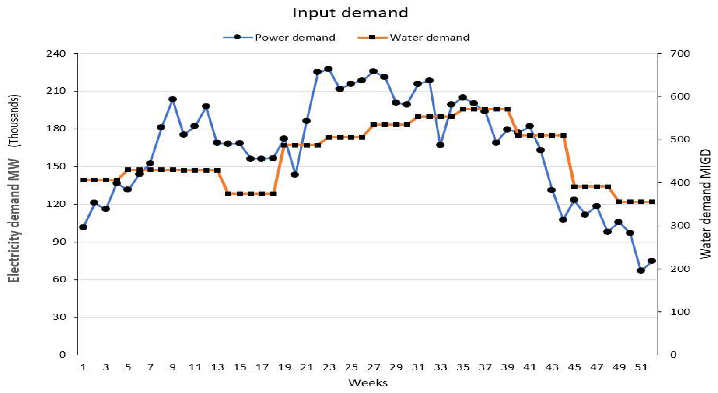
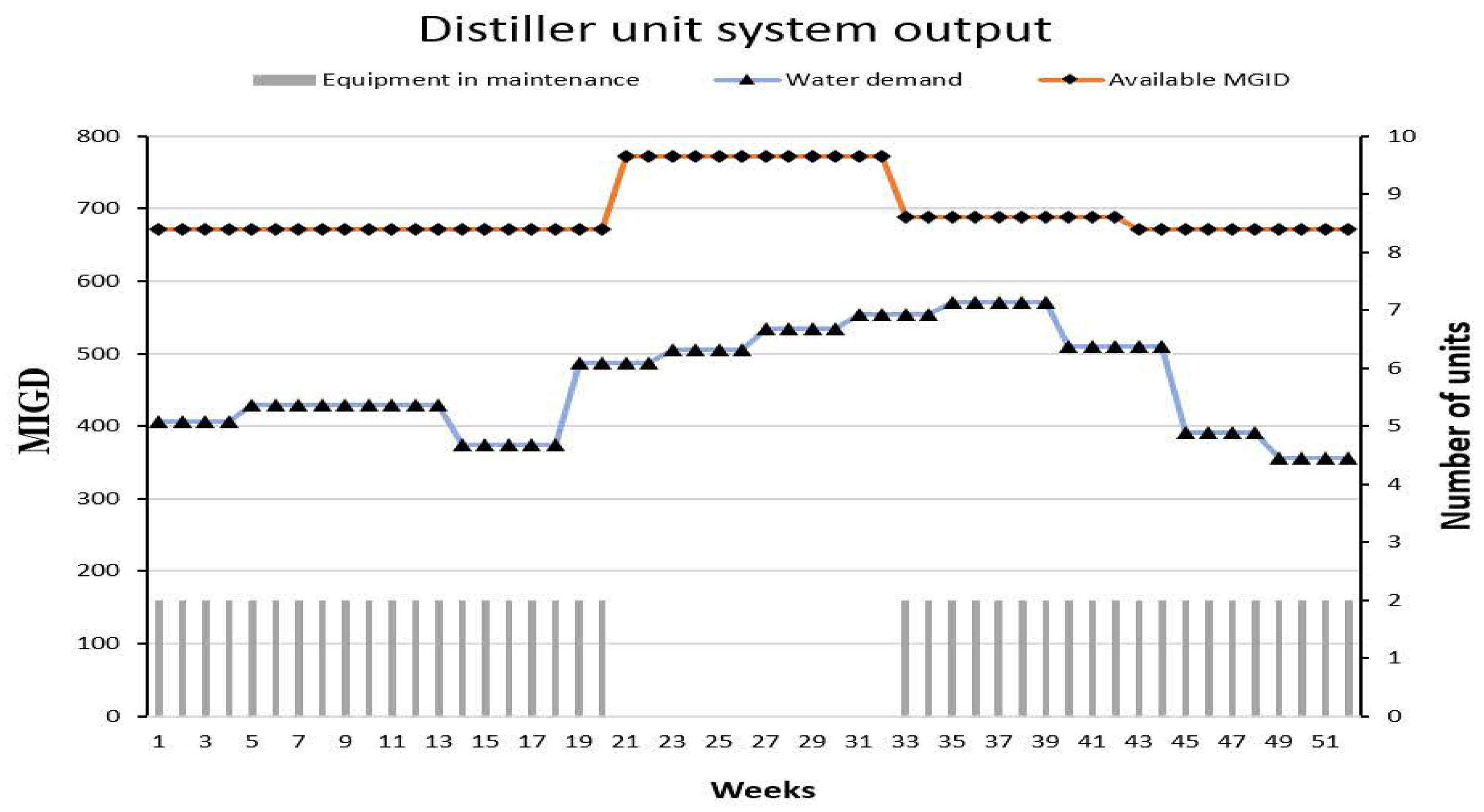
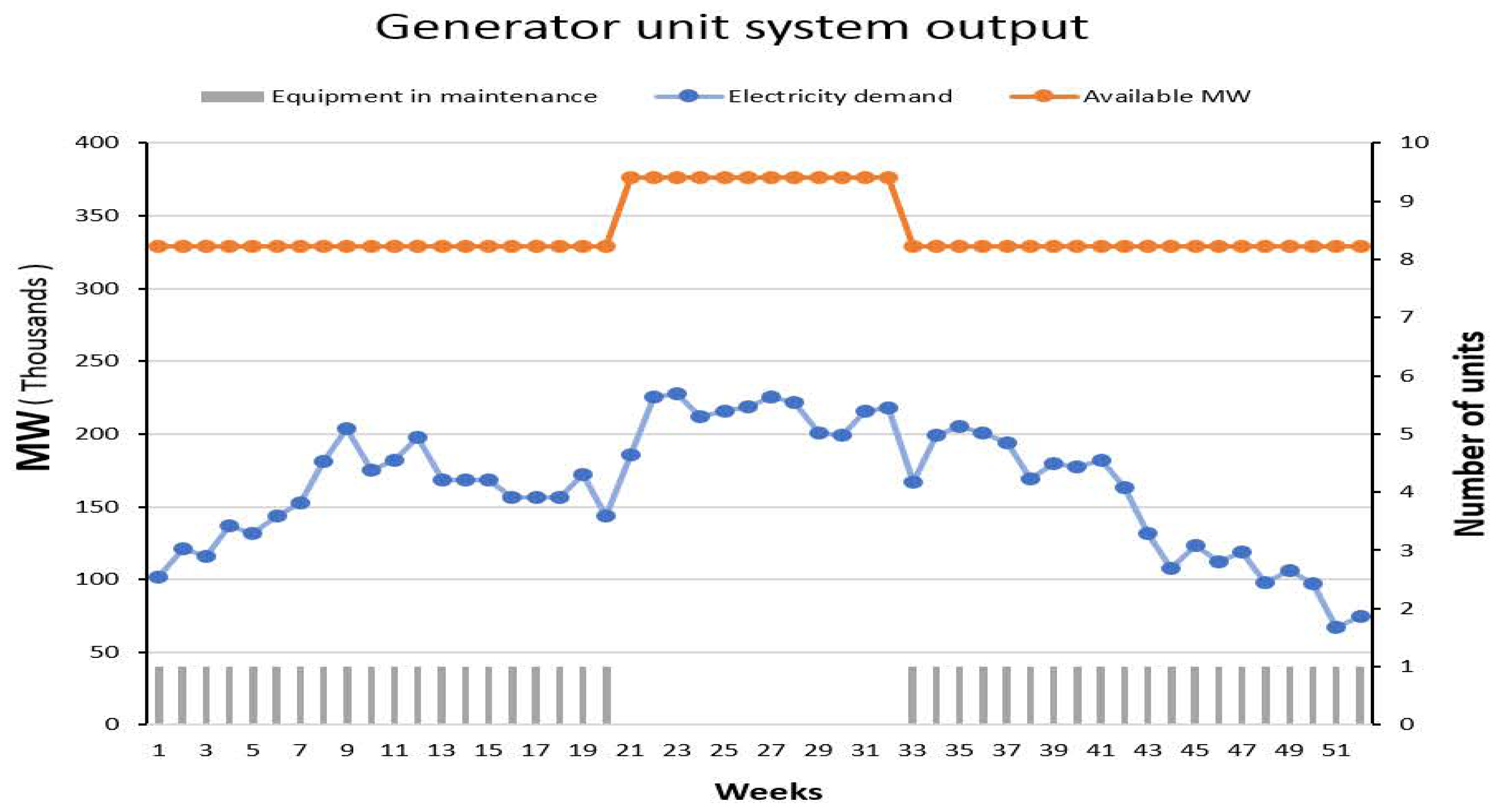
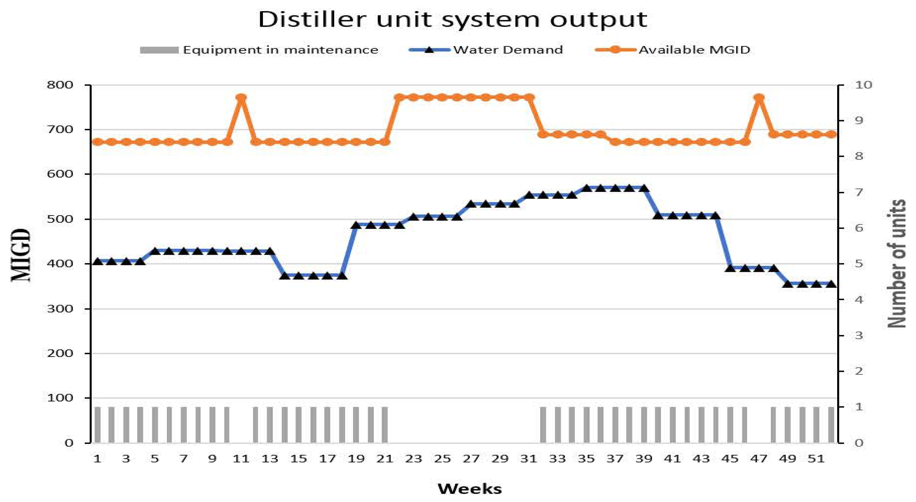
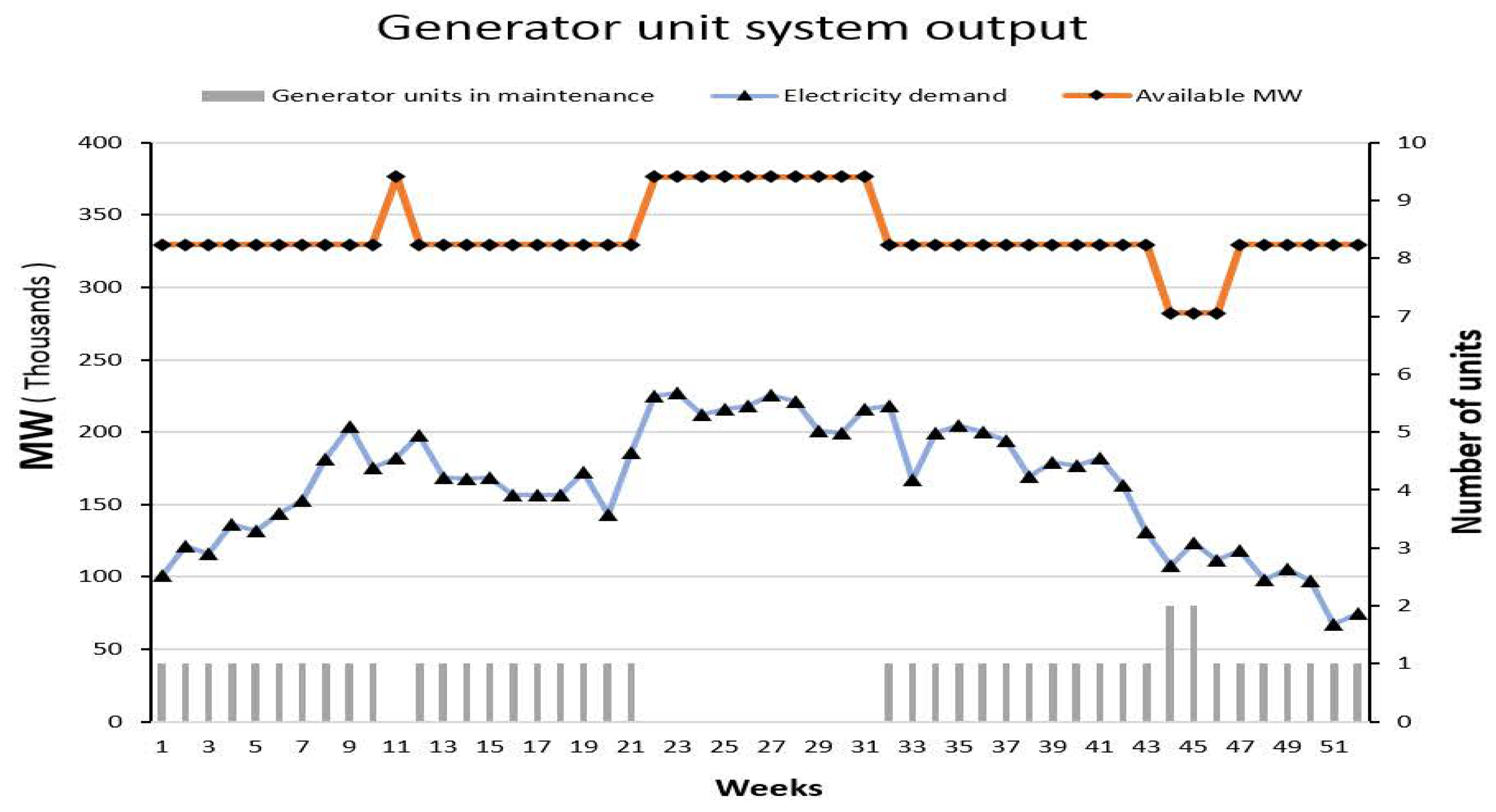
Using these variables, the problem is formulated as follows.

$$\begin{array}{c}\hfill {\displaystyle maxz=\frac{{\gamma }^e}{w^e}+\frac{{\gamma }^t}{w^w}}\end{array}$$

(1)

$$\begin{array}{cc}\hfill \mathrm{subject} \mathrm{to}\sum _{t={\underline{s}}_{e_u}}^{\overline{e_u}}{x}_{e_{u}t}=1& u\in U,e_u\in E\end{array}$$

(2)

$$\begin{array}{cc}\hfill {\displaystyle y_{e_u}=\sum _{t={\underline{s}}_{e_u}}^{\overline{e_u}}t{x}_{e_{u}t}}& u\in U,e_u\in E\end{array}$$

(3)

$$\begin{array}{cc}\hfill {\underline{s}}_{e_u}\le y_{e_u}\le {\overline{s}}_{e_u}& u\in U,e_u\in E\end{array}$$

(4)

$$\begin{array}{cc}\hfill \sum _{t^{\prime }=t}^{t+{\tau }_{e_u}-1}{z}_{e_u{t}^{\prime }}\ge {\tau }_{e_u}{x}_{e_u{t}^{\prime }}& u\in U,e_u\in E,t={\underline{s}}_{e_u},\dots ,{\overline{s}}_{e_u}\end{array}$$

(5)

$$\begin{array}{cc}\hfill \sum _{t={\underline{s}}_{e_u}}^{{\overline{s}}_{e_u}+{\tau }_{e_u}}{z}_{e_{u}t}={\tau }_{e_u}& u\in U,e_u\in E\end{array}$$

(6)

$$\begin{array}{cc}\hfill z_{b_{u}t}\le 1-a_{r_{u}t}& u\in U,t\in T\end{array}$$

(7)

$$\begin{array}{cc}\hfill z_{b_{u}t}\le 1-a_{d_{u}t}& u\in U,t\in T\end{array}$$

(8)

$$\begin{array}{cc}\hfill z_{r_{u}t}+z_{d_{u}t}\le 2-a_{b_{u}t}& u\in U,t\in T\end{array}$$

(9)

$$\begin{array}{cc}\hfill {\displaystyle \sum _{e_u\in E}{z}_{e_{u}t}\le {\ell }_u}& t\in T\end{array}$$

(10)

$$\begin{array}{cc}\hfill {\displaystyle \sum _{u\in U}\sum _{r\in R}{p}_{r_u}(1-z_{r_{u}t})={\delta }_t^e+g_t^e}& t\in T\end{array}$$

(11)

$$\begin{array}{cc}\hfill {\displaystyle \sum _{u\in U}\sum _{d\in D}{p}_{d_u}(1-z_{d_{u}t})={\delta }_t^w+g_t^w}& t\in T\end{array}$$

(12)

$$\begin{array}{cc}\hfill g_t^e\ge {\gamma }^e& t\in T\end{array}$$

(13)

$$\begin{array}{cc}\hfill g_t^w\ge {\gamma }^w& t\in T\end{array}$$

(14)

$$\begin{array}{cc}\hfill {\displaystyle \underline{\ell }\le {\ell }_0+\sum _{t^{\prime }=1}^t{g}_t^w\le \overline{\ell }}& t\in T\end{array}$$

(15)

$$\begin{array}{cc}\hfill {\displaystyle \sum _{u\in U}\sum _{e_u\in U}{m}_{e_u}{z}_{e_{u}t}\le {\overline{m}}_t}& t\in T\end{array}$$

(16)

$$\begin{array}{cc}\hfill x_{e_{u}t}\in \{0,1\},z_{e_{u}t}\in \{0,1\},a_{e_{u}t}\in \{0,1\}& u\in U,e_u\in E,t\in T\end{array}$$

(17)

$$\begin{array}{cc}\hfill g_t^e\ge 0,g_t^w\ge 0& t\in T\end{array}$$

(18)

$$\begin{array}{cc}\hfill y_{e_u}\in \mathbb{N}& u\in U\end{array}$$

(19)

$$\begin{array}{c}\hfill {\gamma }^e\ge 0,{\gamma }^w\ge 0.\end{array}$$

(20)

Equation (1) maximizes the sum of the minimal relative surpluses of water and electricity with respect to their yearly production capacity. Equation (2) specifies that equipment $e_u$ of unit $u\in U$ must undergo a single PM during its time window. Equation (3) calculates the PM starting time of equipment $e_u$ of unit $u\in U$. Equation (4) further constrains this starting time to time window $[{\underline{s}}_{e_u},{\overline{s}}_{e_u}]$. Equation (5) marks $e_u$ of unit $u\in U$ under maintenance during all time periods $t,\dots ,t+{\tau }_{e_u}$ if a PM starts at time t, and is redundant otherwise. Along with Equation (6), it ensures that the maintenance of $e_u$ of unit $u\in U$ lasts exactly ${\tau }_{e_u}$ time units and that it is not interrupted. Equations (7) and (8) reinforce the non-availability of the turbine and distiller of a unit $u\in U$ when their boiler is under maintenance. Equation (9) guarantees that the PM of either a turbine or a distiller of a unit u does not cause the unavailability of the boiler, while their simultaneous PM causes the boiler’s unavailability. Equation (10) indicates that during any period $t\in T$, at most, ${\ell }_u$ equipment may be in maintenance. Equation (11) forces the electricity production during period $t\in T$ to exceed the demand ${\delta }_t^e$ and determines this excess demand $g_t^e$. Similarly, Equation (12) forces the water production during period $t\in T$ to exceed the demand ${\delta }_t^w$ and determines this excess demand, $g_t^w$. Equations (13) and (14) set a minimal threshold level on the excess production of electricity and water for a period $t\in T$, while Equation (15) ensures that the level of the water reservoirs remains within its tolerance levels $\underline{\ell }$ and $\overline{\ell }$ during any period $t\in T$. Equation (16) constrains the manpower used for the scheduled PMs to the available manpower during period t. Finally, Equations (17)–(20) define the decision variables’ type. The resulting MP is a mixed integer program.

4. Case Study

MP is solved using the mixed integer programming solver CPLEX 12.9.0 on an HP desktop computer i7-6700, 3.40 MHz and 64.0 RAM. It is tested on a real case study, provided by MEW of the state of Kuwait. The case considers a plant with 8 units, each consisting of one boiler, two distillers, and one turbine. It designs a PMS for 32 equipment over a 52-week planning horizon. The demand for electricity and water during this planning period is given in Figure 1.

During the $T=52$-week time horizon, any equipment may have its PM as early as the first week and as late as week 52. In fact, additional maintenance manpower may be outsourced from the local market. However, no more than two equipment of a same type can undergo PM, i.e., the following:

$$\begin{array}{cc}\hfill {\displaystyle \sum _{u\in U}{z}_{e_{u}t}\le 2,}& t\in T,e_u=r_u,b_u,d_u.\hfill \end{array}$$

(21)

The weekly production of a distiller of unit $u=1,\dots ,6$ is 50.4 million gallons (MG) but only 40.2 MG for a distiller of unit $u=7$ or 8. A turbine’s weekly production is 47,040 megawatts (MW). It follows that the ratio $w=\frac{w^e}{w^w}$ of the yearly production capacity of electricity to the yearly production capacity of water equals 487. MEW prohibits maintenance activities during the summer months, i.e., for $t\in \{20,\dots ,32\}$. For either a distiller or a boiler, the duration of a PM is five weeks, while it is four weeks for a turbine. In the following, we first compare the schedules generated by MP and by MEW experts. Second, we study the sensitivity of the results to the problem’s parameters.

4.1. Solution Quality

For this case study, MP has 10,194 variables (with 9952 binary) and 20,852 constraints. CPLEX solves MP within 157 s. This negligible runtime is far less than the time it takes a human expert to generate any schedule, let alone a schedule that maximizes the minimum gap. Figure 2 and Figure 3 display the MP solution. They display the production, demand and number of units under maintenance.

Based on Figure 2 and Figure 3, the number of distillers and turbines under maintenance is constant whenever maintenance is allowed. Thus, the production of both water and electricity is constant during the first 20 weeks. It peaks when demand increases and maintenance activities stop. By the end of summer, the maintenance activities restart, restoring production to its previous levels while demand decreases steadily. Excess production is largest during the winter, but ensures a large backup level and avoids water shortages and power outages. It equals 118.1 MG for water and 124,426 MW for electricity. The total production is 36,321.6 MG of water and 17,687,040 MW of electricity.

The comparison of Figure 2 and Figure 3 to their MEW’s PMS of Figure 4 and Figure 5 shows that our model schedules more PMs for distillers than MEW’s experts. In addition, MP has a steadier production than MEW’s PMS. These differences are further evidenced in

Table 1. PMS generated by the proposed model and by MEW.

Week	Proposed Model		MEW
	Equipment under PM	Idle	Equipment under PM	Idle
1	B-6, D1-6, D2-6, T-6	-	B-4, D1-4, D2-4	T-4
2	B-6, D1-6, D2-6, T-6	-	B-4, D1-4, D2-4, T-4	-
3	B-6, D1-6, D2-6, T-6	-	B-4, D1-4, D2-4, T-4	-
4	B-6, D1-6, D2-6, T-6	-	B-4, D1-4, D2-4, T-4	-
5	B-6, D1-6, D2-6	T-6	B-4, D1-4, D2-4, T-4	-
6	B-5, D1-5, D2-5	T-5	B-3, D1-3, D2-3, T-3	-
7	B-5, D1-5, D2-5, T-5	-	B-3, D1-3, D2-3, T-3	-
8	B-5, D1-5, D2-5, T-5	-	B-3, D1-3, D2-3, T-3	-
9	B-5, D1-5, D2-5, T-5	-	B-3, D1-3, D2-3, T-3	-
10	B-5, D1-5, D2-5, T-5	-	B-3, D1-3, D2-3	T-3
11	B-3, D1-3, D2-3	T-3	-	-
12	B-3, D1-3, D2-3, T-3	-	B-6, D1-6, D2-6, T-6	-
13	B-3, D1-3, D2-3, T-3	-	B-6, D1-6, D2-6, T-6	-
14	B-3, D1-3, D2-3, T-3	-	B-6, D1-6, D2-6, T-6	-
15	B-3, D1-3, D2-3, T-3	-	B-6, D1-6, D2-6, T-6	-
16	B-2, D1-2, D2-2	T-2	B-6, D1-6, D2-6	T-6
17	B-2, D1-2, D2-2, T-2	-	B-5, D1-5, D2-5, T-5	-
18	B-2, D1-2, D2-2, T-2	-	B-5, D1-5, D2-5, T-5	-
19	B-2, D1-2, D2-2, T-2	-	B-5, D1-5, D2-5, T-5	-
20	B-2, D1-2, D2-2, T-2	-	B-5, D1-5, D2-5, T-5	-
21	-	-	B-5, D1-5, D2-5	T-5
22	-	-	-	-
23	-	-	-	-
24	-	-	-	-
25	-	-	-	-
26	-	-	-	-
27	-	-	-	-
28	-	-	-	-
29	-	-	-	-
30	-	-	-	-
31	-	-	-	-
32	-	-	B-7, D1-7, D2-7	T-7
33	B-8, D1-8, D2-8	T-8	B-7, D1-7, D2-7	T-7
34	B-8, D1-8, D2-8, T-8	-	B-7, D1-7, D2-7	T-7
35	B-8, D1-8, D2-8, T-8	-	B-7, D1-7, D2-7	T-7
36	B-8, D1-8, D2-8, T-8	-	B-7, D1-7, D2-7	T-7
37	B-8, D1-8, D2-8, T-8	-	B-2, D1-2, D2-2	T-2
38	B-7, D1-7, D2-7	T-7	B-2, D1-2, D2-2, T-2	-
39	B-7, D1-7, D2-7, T-7	-	B-2, D1-2, D2-2, T-2	-
40	B-7, D1-7, D2-7, T-7	-	B-2, D1-2, D2-2, T-2	-
41	B-7, D1-7, D2-7, T-7	-	B-2, D1-2, D2-2, T-2	-
42	B-7, D1-7, D2-7, T-7	-	B-1, D1-1, D2-1, T-1	-
43	B-4, D1-4, D2-4, T-4	-	B-1, D1-1, D2-1, T-1	-
44	B-4, D1-4, D2-4, T-4	-	B-1, D1-1, D2-1,T-1,T-7	-
45	B-4, D1-4, D2-4, T-4	-	B-1, D1-1, D2-1,T-1,T-7	-
46	B-4, D1-4, D2-4, T-4	-	B-1, D1-1, D2-1,T-7	T-1
47	B-4, D1-4, D2-4	T-4	T-7	-
48	B-1, D1-1, D2-1, T-1	-	B-8, D1-8, D2-8, T-8	-
49	B-1, D1-1, D2-1, T-1	-	B-8, D1-8, D2-8, T-8	-
50	B-1, D1-1, D2-1, T-1	-	B-8, D1-8, D2-8, T-8	-
51	B-1, D1-1, D2-1, T-1	-	B-8, D1-8, D2-8, T-8	-
52	B-1, D1-1, D2-1	T-1	B-8, D1-8, D2-8	T-8

, which displays the PMS of MP and MEW. Table 1 confirms the satisfaction of all constraints. For instance, no more than two pieces of equipment of a given type are under PM during any of the 52 weeks of the planning horizon. Similarly, neither a distiller nor a turbine are operational when their boiler is under PM.

Even though MEW’s water production matches MP’s water production, the electricity production is 1.1% smaller at 17,498,880 MW. In fact, MEW idles the turbines for 12 weeks, whereas MP reduces the turbines’ idleness to 8 weeks. MEW makes T-7 idle (even though T-7 is not under maintenance) during weeks 32–36 (because B-7 is under maintenance), while T-7 undergoes its PM during weeks 44–47.

MP outperforms MEW’s experts in terms of water and electricity excess productions: it increases these excesses by 16.58% and 12.12%, i.e., MEW’s water and electricity excess production equal 101.3 MG and 110,971 MW, respectively. Recall that the larger the excess production, the more robust the demand satisfaction. It makes the system less prone to unforeseen events that may randomly occur on the network. In addition to these observed differences, MEW’s PMS has a very low production surplus during weeks 37–39, with demand almost equaling total production as shown in Figure 4 and Figure 5. This situation is quite risky, as it could lead to water shortages during unusually hot days. Moreover, MEW’s PMS is not leveled, with an interruption during week 11 and only one piece of equipment under maintenance in week 47. This is undesirable: it creates undue costs to contractors who have to pay for idle (resp. supplementary) manpower during low (resp. peak) maintenance activities. MP avoids such undue costs to contractors.

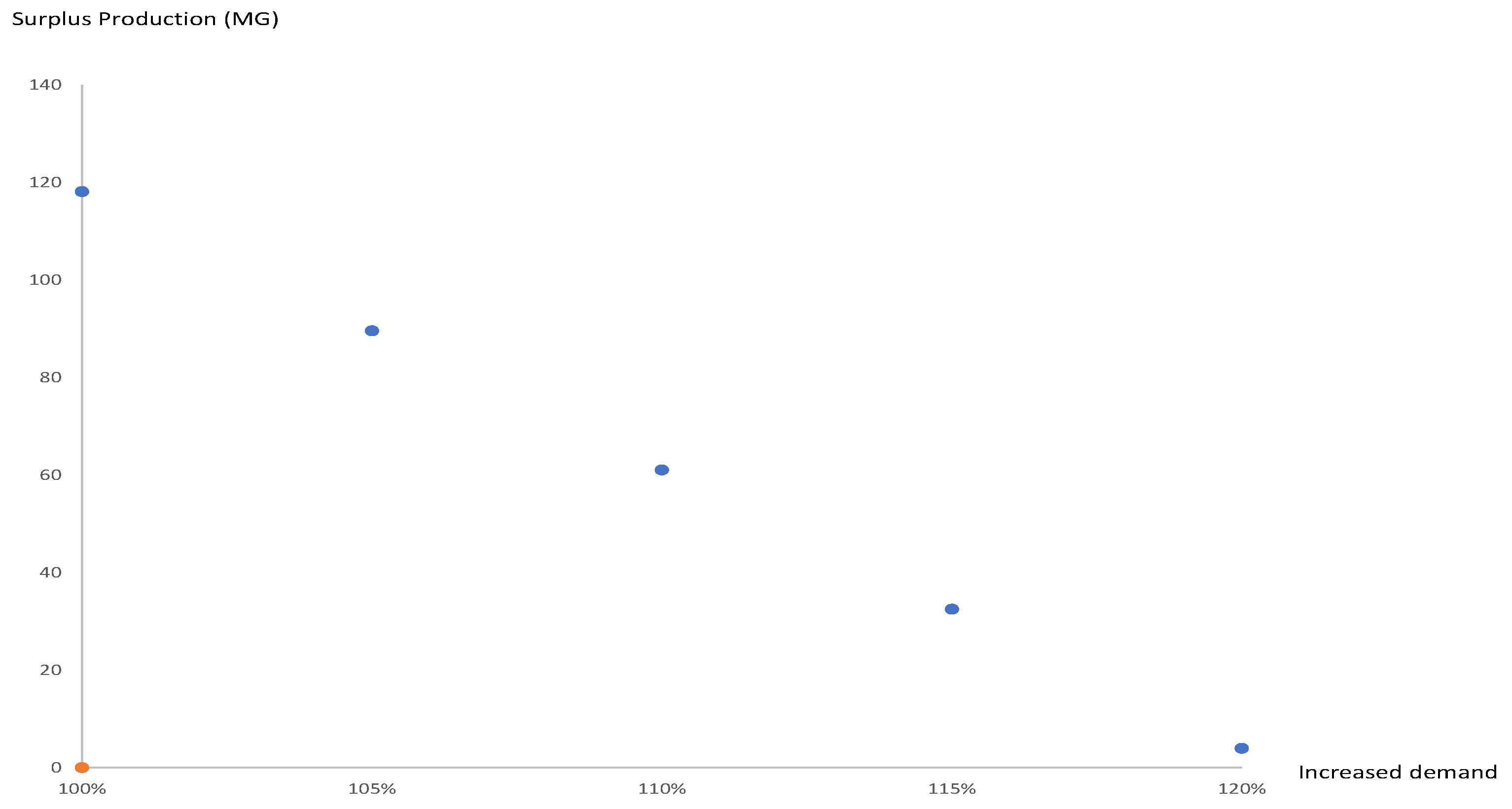
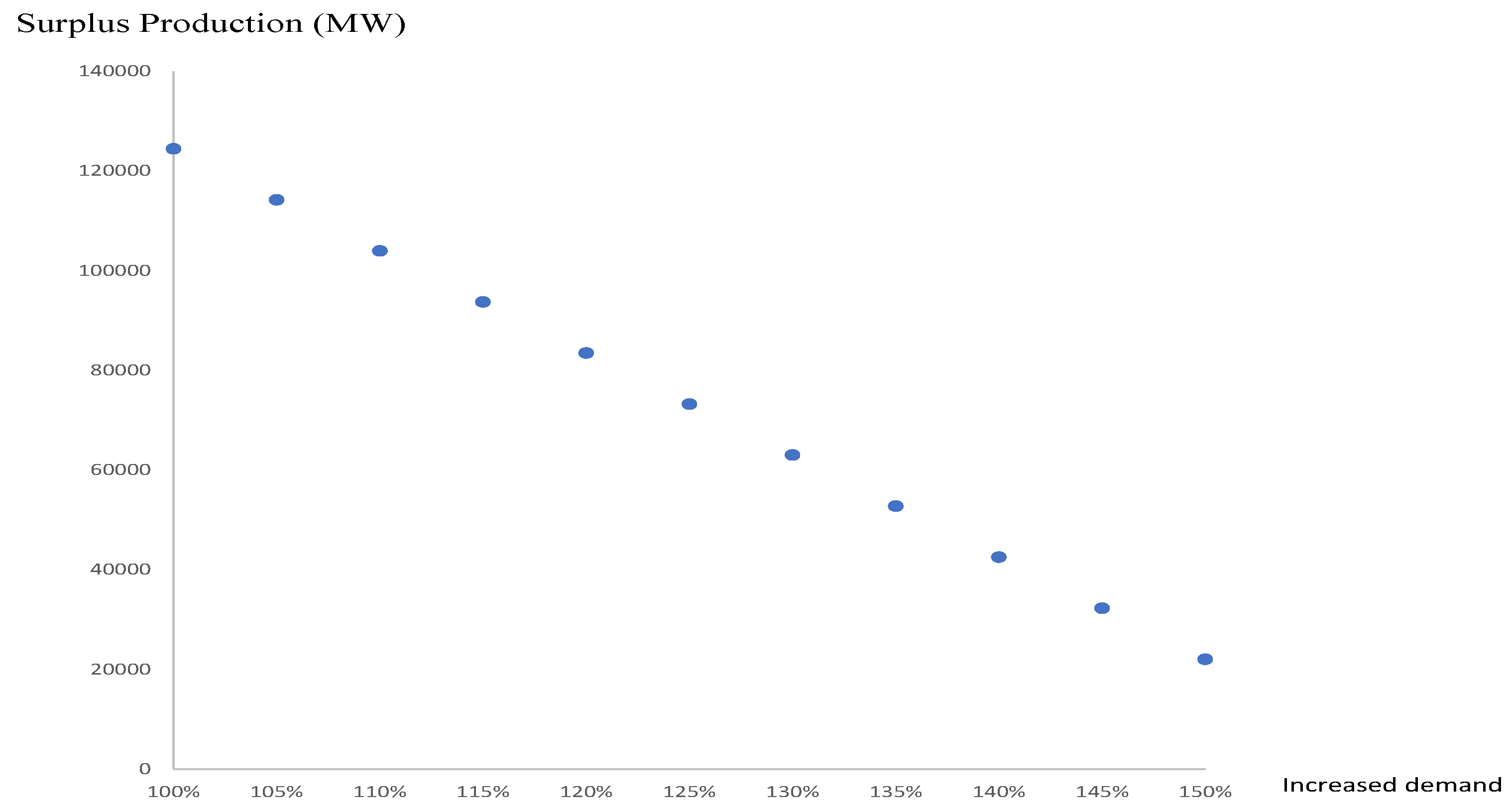
4.2. Sensitivity Analysis

We study the sensitivity of the generated PMS to (i) demand and to (ii) both demand and the duration of a PM. First, we increase the demand of both water and electricity. Figure 6 and Figure 7 illustrate MP’s resulting surplus production as demand increases. In all considered cases, MP’s optimal PMS satisfies the increased demand over the epochs of the time horizon. Further increasing demand may result in infeasible solutions, that is, it would be impossible to maintain the equipment while still satisfying demand. These cases are generally handled by rerouting demand through different networks.

Second, we study the sensitivity of the generated PMS to both demand and the duration of a PM. We increase the demand by 120% and the duration of a PM by one week. In addition, we add a couple of technical restrictions.

• If the PMs of the second distiller and of the turbine of unit 4 start a PM during period $t\in T$, then the PM of the first distiller must also begin during the same period.

  $$\begin{array}{c}\hfill x_{d_4^{2}t}+x_{r_{4}t}\le x_{d_{4}t}^{″}+1.\end{array}$$

  (22)
• The time windows of the PM starting times of certain equipment are now restricted. For example, the PM of the first distiller of unit 8 cannot start before week 40, whereas that of the second distiller of unit 7 must start between week 15 and week 40.

MP has again 10,194 variables (with 9952 binary) but more constraints, with 20,904 in lieu of 20,852 constraints. The additional constraints reduce the search space of CPLEX, which solves the restricted model within 143 s—less than the time of the original model. In fact, adding constraints makes the problem easier to solve for CPLEX, while it makes it more complicated for a human expert.

Table 2. A more restricted PMS.

Week	Equipment under PM	Idle	Week	Equipment under PM	Idle
1	B-3, D1-3, D2-3, T-3	-	27	B-5, D1-5, D2-5	T-5
2	B-3, D1-3, D2-3, T-3	-	28	B-4, D1-4, D2-4, T-4	-
3	B-3, D1-3, D2-3, T-3	-	29	B-4, D1-4, D2-4, T-4	-
4	B-3, D1-3, D2-3, T-3	-	30	B-4, D1-4, D2-4, T-4	-
5	B-3, D1-3, D2-3, T-3	-	31	B-4, D1-4, D2-4, T-4	-
6	B-3, D1-3, D2-3	T-3	32	B-4, D1-4, D2-4, T-4	-
7	B-6, D1-6, D2-6	T-6	33	B-4, D1-4, D2-4	T-4
8	B-6, D1-6, D2-6, T-6	-	34	B-7, D1-7, D2-7	T-7
9	B-6, D1-6, D2-6, T-6	-	35	B-7, D1-7, D2-7, T-7	-
10	B-6, D1-6, D2-6, T-6	-	36	B-7, D1-7, D2-7, T-7	-
11	B-6, D1-6, D2-6, T-6	-	37	B-7, D1-7, D2-7, T-7	-
12	B-6, D1-6, D2-6, T-6	-	38	B-7, D1-7, D2-7, T-7	-
13	-	-	39	B-7, D1-7, D2-7, T-7	-
14	-	-	40	-	-
15	-	-	41	B-8, D1-8, D2-8	T-8
16	B-1, D1-1, D2-1	T-1	42	B-8, D1-8, D2-8,T-8	-
17	B-1, D1-1, D2-1, T-1	-	43	B-8, D1-8, D2-8,T-8	-
18	B-1, D1-1, D2-1, T-1	-	44	B-8, D1-8, D2-8,T-8	-
19	B-1, D1-1, D2-1, T-1	-	45	B-8, D1-8, D2-8,T-8	-
20	B-1, D1-1, D2-1, T-1	-	46	B-8, D1-8, D2-8,T-8	-
21	B-1, D1-1, D2-1, T-1	-	47	B-2, D1-2, D2-2,T-2	-
22	B-5, D1-5, D2-5, T-5	-	48	B-2, D1-2, D2-2,T-2	-
23	B-5, D1-5, D2-5, T-5	-	49	B-2, D1-2, D2-2,T-2	-
24	B-5, D1-5, D2-5, T-5	-	50	B-2, D1-2, D2-2,T-2	-
25	B-5, D1-5, D2-5, T-5	-	51	B-2, D1-2, D2-2,T-2	-
26	B-5, D1-5, D2-5, T-5	-	52	B-2, D1-2, D2-2	T-2

shows the resulting restricted PMS for all equipment. The excess production for water and electricity equals 3.96 MG for water and 56,394 MW for electricity. These levels are far from those previously observed (i.e., 118.1 MG for water and 124,426 MW for electricity). The change in the total production is, on the other hand, much smaller—35,548.8 MG of water and 17,310,730 MW of electricity in lieu of 36,321.6 MG of water and 17,687,040 MW of electricity.

5. Conclusions

Preventive maintenance scheduling is a critical issue in energy systems. It aims at increasing energy efficiency while ensuring the systems’ reliability, safety, security and robustness against unexpected events. This paper proposes a mathematical program to plan maintenance events, and illustrates its application on real-life data provided by the Ministry of Electricity and Water of the State of Kuwait. The mathematical program maximizes the sum of the minimal relative surpluses of water and electricity with respect to their yearly production capacity. This translates into satisfying demand for water and electricity all along the planning horizon while ensuring a safety net for shortages in the event of equipment breakdown. The mathematical program obtains a feasible preventive maintenance schedule that improves the surplus production of water by 16.58% and of electricity by 12.12%. In addition, it increases electricity production of the current used system by 1.1%. The sensitivity analysis of the maintenance plan infers its robustness with respect to the increased production, maintenance duration, additional restrictions on concurrent maintenance of equipment, and tighter time windows.

The proposed mathematical program is not specific to a given power plant. It can be extended to cover the whole grid. In the case that the optimizer fails to converge to the global optimum, heuristic approaches can then be used. The proposed model can be adapted to other areas, such as the maintenance of oil wells. These applications may involve nonlinear constraints and quadratic objective functions.

References

1. Cullum, J.; Binns, J.; Lonsdale, M.; Abbassi, R.; Garaniya, V. Risk-Based Maintenance Scheduling with application to naval vessels and ships. Ocean. Eng. 2018, 148, 476–485. [Google Scholar] [CrossRef]
2. Sharma, A.; Yadava, G.S.; Deshmukh, S.G. A literature review and future perspectives on maintenance optimization. J. Qual. Maint. Eng. 2011, 17, 5–25. [Google Scholar] [CrossRef]
3. Lair, W.; Mercier, S.; Roussignol, M.; Ziani, R. Piecewise deterministic Markov processes and maintenance modeling: Application to maintenance of a train air-conditioning system. Proc. Inst. Mech. Eng. Part J. Risk Reliab. 2011, 225, 199–209. [Google Scholar] [CrossRef]
4. Lassoued, B.; M’Hallah, R. Daily parking of subway vehicles. Lect. Notes Artif. Intell. 1998, 1416, 857–866. [Google Scholar]
5. Safaei, N.; Banjevic, D.; Jardine, A.K.S. Workforce-constrained maintenance scheduling for military aircraft fleet: A case study. Ann. Oper. Res. 2011, 186, 295–316. [Google Scholar] [CrossRef]
6. Laalaoui, Y.; M’Hallah, R. A binary multiple knapsack model for single machine scheduling with machine unavailability. Comput. Oper. Res. 2016, 72, 71–82. [Google Scholar] [CrossRef]
7. Ruiz-Torres, A.J.; Paletta, G.; M’Hallah, R. Makespan minimisation with sequence-dependent machine deterioration and maintenance events. Int. J. Prod. Res. 2017, 55, 462–479. [Google Scholar] [CrossRef]
8. Wangnick, K. IDA Worldwide Desalting Plants Inventory Report No. 14. Int. Desalin. Water Reuse Q. 1996, 6, 55–59. [Google Scholar]
9. Xi, Z. Texas Blackout: Facts and a Power Engineer’s Perspective. In IISE Energy Systems Division Webinar; Springer: Berlin, Germany, 2021. [Google Scholar]
10. Yang, Z.M.; Djurdjanovic, D.; Ni, J. Maintenance scheduling in manufacturing systems based on predicted machine degradation. J. Intell. Manuf. 2008, 19, 87–98. [Google Scholar] [CrossRef]
11. Alardhi, M.; Labib, A.W. Preventive maintenance scheduling of multi-cogeneration plants using integer programming. J. Oper. Res. Soc. 2008, 59, 503–509. [Google Scholar] [CrossRef]
12. Ramírez-Martínez, M.V.; Martínez-Sánchez, A.M.; Escobar-Zuluaga, A.H.; Gadelha-Guimarães, F. Maintenance of generation units coordinated with annual hydrothermal scheduling using a hybrid technique. Rev. Fac. Ing. Univ. Antioq. 2017, 85, 18–32. [Google Scholar] [CrossRef]
13. Balaji, G.B.R.; Lakshminarasimman, L. Mathematical approach assisted differential evolution for generator maintenance scheduling. J. Abbr. 2008, 10, 142–149. [Google Scholar] [CrossRef]
14. Guedes, L.S.M.; Vieira, D.A.G.; Lisboa, A.C.; Saldanha, R.R. A continuous compact model for cascaded hydro-power generation and preventive maintenance scheduling. Int. J. Electr. Power Energy Syst. 2015, 73, 702–710. [Google Scholar] [CrossRef]
15. Perez-Canto, S.; Rubio-Romero, J.C. A model for the preventive maintenance scheduling of power plants including wind farms. Reliab. Eng. Syst. Saf. 2013, 119, 67–75. [Google Scholar] [CrossRef]
16. Alhamad, K.; Alardhi, M.; Almazrouee, A. Preventive maintenance scheduling for multicogeneration plants with production constraints using genetic algorithms. Adv. Oper. Res. 2015, 2015, 282178. [Google Scholar] [CrossRef]
17. Bos, M.F.J.; Beune, R.J.L.; Van Amerongen, R.A.M. On the incorporation of a heat storage device in Lagrangian relaxation based algorithms for unit commitment. Int. J. Electr. Power Energy Syst. 1996, 18, 207–214. [Google Scholar] [CrossRef]
18. Canto, S.P. Application of Benders’ decomposition to power plant preventive maintenance scheduling. Eur. J. Oper. Res. 2008, 184, 759–777. [Google Scholar] [CrossRef]
19. El-Amin, I.; Duffuaa, S.; Abbas, M. A tabu search algorithm for maintenance scheduling of generating units. Electr. Power Syst. Res. 2000, 54, 91–99. [Google Scholar] [CrossRef]
20. Alardhi, M.; Hannam, R.G.; Labib, A.W. Preventive maintenance scheduling for multi-cogeneration plants with production constraints. J. Qual. Maint. Eng. 2007, 13, 276–292. [Google Scholar] [CrossRef]
21. Alhamad, K.; Alhajri, M. A zero-one integer programming for preventive maintenance scheduling for electricity and distiller plants with production. J. Qual. Maint. Eng. 2019, 26, 555–574. [Google Scholar] [CrossRef]
22. Ferdowsi, F.; Maleki, H.R.; Rivaz, S. Air refueling tanker allocation based on a multi-objective zero-one integer programming model. Oper. Res. 2020, 20, 1913–1938. [Google Scholar] [CrossRef]
23. Moirangthem, J.; Dash, S.S.; Ramaswami, R. Zero-one integer programming approach to determine the minimum break point set in multi-loop and parallel networks. J. Electr. Eng. Technol. 2012, 7, 151–156. [Google Scholar] [CrossRef] [Green Version]
24. Moslehi, K.; Khadem, M.; Bernal, R.; Hernandez, G. Optimization of multiplant cogeneration system operation including electric and steam networks. IEEE Trans. Power Syst. 1991, 6, 484–490. [Google Scholar] [CrossRef]
25. Wang, C.H.; Wang, J. Combining fuzzy AHP and fuzzy Kano to optimize product varieties for smart cameras: A zero-one integer programming perspective. Appl. Soft Comput. 2014, 22, 410–416. [Google Scholar] [CrossRef]
26. Alidaee, B.; Wang, H. Preventive maintenance scheduling of multi-cogeneration plants using integer programming. J. Oper. Res. Soc. 2009, 60, 1295–1297. [Google Scholar] [CrossRef]
Figure 1. Demand for electricity and water.
Mathematics 09 01705 g001
Figure 2. MP water production versus demand.
Mathematics 09 01705 g002
Figure 3. MP electricity production versus demand.
Mathematics 09 01705 g003
Figure 4. MEW water production versus demand.
Mathematics 09 01705 g004
Figure 5. MEW electricity production versus demand.
Mathematics 09 01705 g005
Figure 6. Water surplus production versus increased demand.
Mathematics 09 01705 g006
Figure 7. Electricity surplus production versus increased demand.
Mathematics 09 01705 g007