Determination of Optimal Diffusion Coefficients in Lake Zirahuén through a Local Inverse Problem

Abstract

In this study, optimal diffusion coefficients for Lake Zirahuén, Mexico, were found under particular conditions based on images taken with a drone of a dye release experiment. First, the dye patch concentration was discretized using image processing tools, and it was then approximated by an ellipse, finding the optimal major and minor axes. The inverse problem was implemented by comparing these observational data with the concentration obtained numerically from the 2D advection–diffusion equation, varying the diffusion tensor. When the tensor was isotropic, values of $K_{11}=K_{22}\approx 0.003{ \mathrm{m}}^2/\mathrm{s}$ were found; when nonequal coefficients were considered, it was found that $K_{11}\approx 0.005{ \mathrm{m}}^2/\mathrm{s}$ and $K_{22}\approx 0.002{ \mathrm{m}}^2/\mathrm{s}$, and the cross-term $K_{12}$ influenced the results of the orientation of the ellipse. It is important to mention that, with this simple technique, the parameter estimation had consequences of great importance as the value for the diffusion coefficient was bounded significantly under particular conditions for this site of study.

1. Introduction

Lakes are vitally important components that provide essential ecosystem services, such as water for drinking, and food supply and sites for recreation and tourism [1]. However, the quality of lakes’ water resources is deteriorating rapidly due to the load or spread of pollutants, excessive nutrient inputs, and all types of sediments. In particular, suspended solids affect dissolved oxygen levels and the temperature, interfering with the mixing and decreasing the dispersion processes toward deeper layers [2,3,4]. The sediment transport estimation is often difficult, time-consuming, and expensive [5]. Nonetheless, observations and monitoring are important aspects of ecosystem services that can be used to map the distribution of sediments and can also be used as a target for numerical models to predict sediment movement and spreading, in particular, knowing that the diffusion coefficient is essential for the numerical modeling of such transport processes [6,7,8,9].

The transport of pollutants can be described by many factors, including advection, diffusion, dispersion, reaction, dilution or mixing, retardation, and decay. These factors are usually incorporated into transport equations, which describe phenomena such as mass transfer or heat, fluid, waves, and momentum transfer [10,11]. Nevertheless, this equation is usually solved numerically for advection–diffusion terms solely, and such numerical models are frequently implemented with known constant coefficients [10,11].

The parameterizations of a set of coefficients have been the topic of ongoing research, most of it carried out empirically and, more recently, based on theoretical considerations with the use of the inversed problem approach. The use of adequate formulations in inverse modeling has proven to be a highly useful method for estimating these parameters and improving the fit of observational data [11,12,13,14,15]. With the use of parameter estimation for a specified set of data, the numerical modeling of the transport equation can be improved for a particular study site.

Likewise, dye tracers are a highly useful tool to estimate advection–diffusion characteristics implemented to measure several aspects of the transport process, such as to measure certain effluent discharge rates and horizontal dispersion coefficients; it is also used to study circulation patterns and to calibrate–validate numerical models used in the forecast activity [10,16,17,18,19]. Along with dye-tracers, aircraft systems (drones) and image processing tools can be used to visualize the dye plume and provide accurate tools to identify, map, and predict the spread of hazardous agents [18,20,21].

For image processing or pattern recognition, several algorithms have been used to detect objects fitting certain geometrical shapes, such as circles or ellipses, to the images. Although there are several sophisticated algorithms for detecting shapes from images, the least squares method is the most often present in these algorithms [22,23].

In this work, a set of images of a dye tracer patch was used to determine the optimal diffusion coefficients from the advection–diffusion equation. The hypothesis was that, based on the inverse problem approach and the observational data of a dye patch, as a proxy for sediment transport, we expected to find optimal diffusion coefficients for the study site and under particular conditions without the involvement of sophisticated measurements to estimate it.

2. Materials and Methods

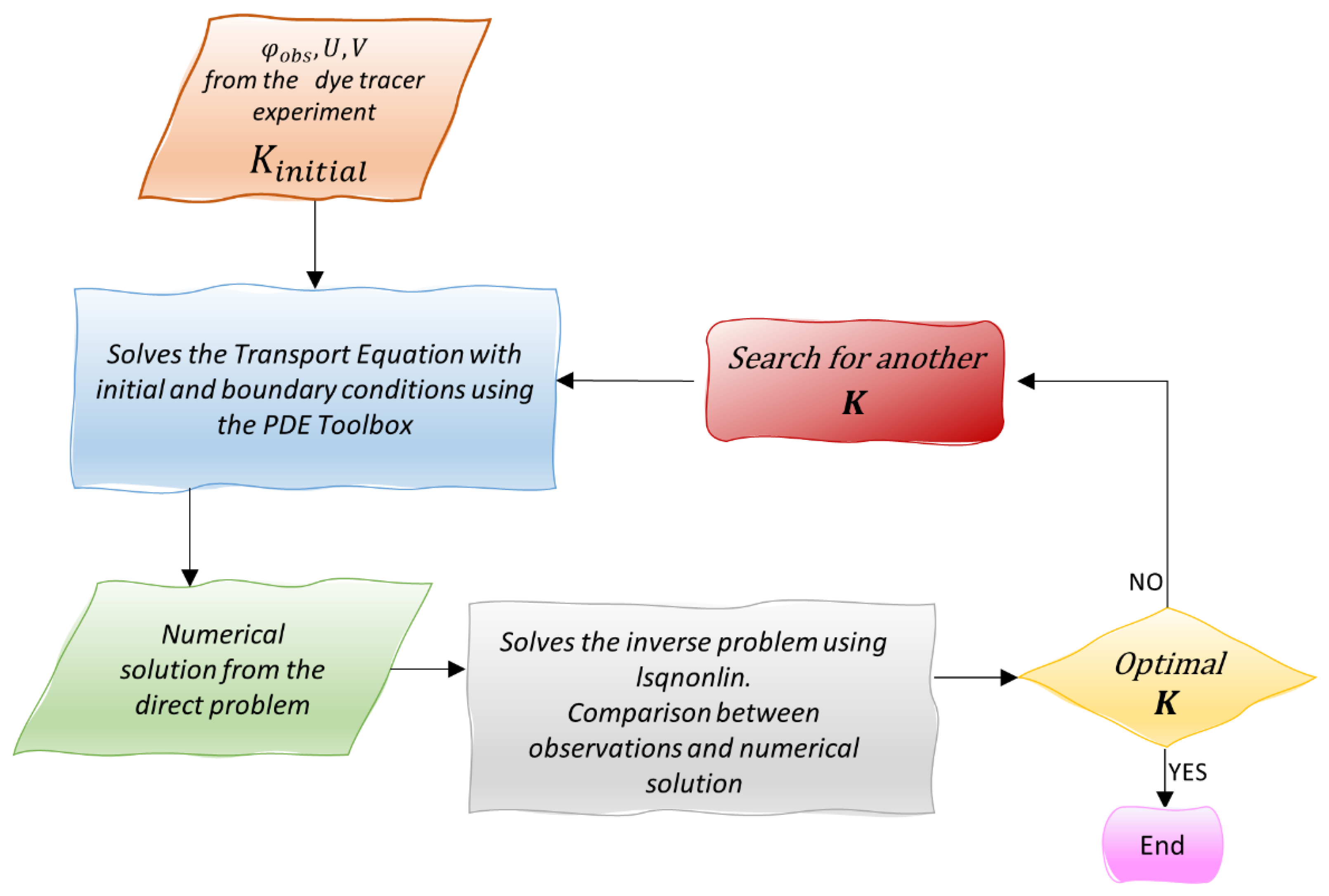
To generate data for solving the advection–diffusion equation, a dye tracer experiment was performed in Lake Zirahuén, Mexico. In general, the methodology applied in this study consists of (i) the estimation of the dye distribution using image processing tools to obtain the area of the dye patch based on an optimization technique, and (ii) the solution of the nonlinear inverse problem for the advection–diffusion equation in order to find the optimal diffusion coefficients by comparing this analytical solution against the observational dye patch distribution; see Figure 1 for an overview and a better understanding of the study.

2.1. The Inverse Problem

To solve the inverse problem, the nonlinear least squares method was used. These problems arise in the context of fitting a parameterized mathematical model to a dataset to minimize an objective function that can be expressed as follows:

$$f\left(\mathit{x}\right)=\frac{1}{2}{\displaystyle \sum }_{i=1}^m{r}_i{\left(\mathit{x}\right)}^2,$$

(1)

where $r_i$ is a smooth function from ${ℝ}^n$ to $ℝ$. Such a minimization problem is derived from curve fitting by least squares, where $f\left(\mathit{x}\right)$ measures the difference between the model and the observational data, i.e., $r_i$ represents the residuals.

Although there are many optimization methods, most of them have the same structure based on Newton’s method. To solve Equation (1), the Levenberg–Marquardt method that combines two algorithms, the gradient descent method and Gauss–Newton method, was implemented. The Levenberg–Marquardt method is more similar to a gradient descent method when the parameter is far from the optimal and works as a Gauss–Newton method when the parameters are close to the optimal [24,25,26,27,28].

2.2. Image Processing and the Inverse Problem to Estimate the Concentration

During a field campaign conducted in July 2018 in Lake Zirahuén, a dye release experiment and an unmanned aerial vehicle (DJI Phantom 4 drone) were used to capture videos and images of a dye plume. Images were captured from 50 m high at a rate of approximately one image every 3 s. In this experiment, natural food colorant (not harmful for the environment) was used as a tracer. The method consisted of the instantaneous release of the dye on the surface used to determine the transport.

Image processing was performed by adjusting the red, green, and blue (RGB) values to increase the contrast of every image and select only the dye plume. Then, working with the binary mask-image and using an edge detection approach, the boundary points of the region were determined to evaluate the extension of the patch. The dye patch area was estimated based on the hypothesis that, after the release, the dye cloud can be approximated by an ellipse, as the natural propagation of the tracer is better characterized by this geometrical form.

To estimate the proposed concentration ellipse (C_e) that fits the dye tracer patch, it was first necessary to find the center and orientation of the data considering the algebraic equation of the general conic to define the minimization problem. In this case, the nonlinear optimization problem was solved for finding the optimal lengths of the major and minor axes.

To obtain the ellipse parameters, we considered only the boundary points, $\left({\zeta }_i,{\eta }_i\right), i=1,2,\dots n$, of the region. Then, if the geometrical center $\left({\zeta }_c,{\eta }_c\right)$ is defined as:

$${\zeta }_c=\frac{1}{n}{\sum }_{i=1}^n{\zeta }_i,{\eta }_c=\frac{1}{n}{\sum }_{i=1}^n{\eta }_i,$$

(2)

Then, based on the variance:

$${\sigma }_{\zeta }^2=\frac{1}{\left(n-1\right)}{\sum }_{i=1}^n{\left({\zeta }_i-{\zeta }_c\right)}^2; {\sigma }_{\eta }^2=\frac{1}{\left(n-1\right)}{\sum }_{i=1}^n{({\eta }_i-{\eta }_c)}^2,$$

(3)

and the covariance:

$${\sigma }_{\zeta \eta }=\frac{1}{\left(n-1\right)}{\displaystyle \sum }_{i=1}^n\left({\zeta }_i-{\zeta }_c\right)\left({\eta }_i-{\eta }_c\right),$$

(4)

the orientation of the principal axes is determined by:

$$\theta =\frac{1}{2}ta{n}^{-1}(2\left({\zeta }_i-{\zeta }_c\right)\left({\eta }_i-{\eta }_c\right)/({\sigma }_{\zeta }^2-{\sigma }_{\eta }^2)),$$

(5)

and the variance in the major and minor axes by:

$$\begin{gathered} {\sigma }_{ma}^2=\frac{{\sigma }_{\zeta }^2+{\sigma }_{\eta }^2}{2}+\sqrt{\frac{{\left({\sigma }_{\zeta }^2+{\sigma }_{\eta }^2\right)}^2}{4}-{\sigma }_{\zeta }^2{\sigma }_{\eta }^2+{\sigma }_{\zeta \eta }{\sigma }_{\zeta \eta }}, \\ {\sigma }_{mi}^2=\frac{{\sigma }_{\zeta }^2+{\sigma }_{\eta }^2}{2}-\sqrt{\frac{{\left({\sigma }_{\zeta }^2+{\sigma }_{\eta }^2\right)}^2}{4}-{\sigma }_{\zeta }^2{\sigma }_{\eta }^2+{\sigma }_{\zeta \eta }{\sigma }_{\zeta \eta }}. \end{gathered}$$

(6)

To calculate the optimal length of the major axis $\left(x_1·{\sigma }_{ma}\right)$ and the minor axis $\left(x_2·{\sigma }_{mi}\right)$, the ellipse equation considered with the center in $\left({\zeta }_c,{\eta }_c\right)$ and $\theta$, the rotation angle:

$$\frac{{(\left(\zeta -{\zeta }_c\right)\cos \theta +\left(\eta -{\eta }_c\right)\sin \theta )}^2}{{\left(x_1·{\sigma }_{ma}\right)}^2}+\frac{{(\left(\zeta -{\zeta }_c\right)\sin \theta -\left(\eta -{\eta }_c\right)\cos \theta )}^2}{{\left(x_2·{\sigma }_{mi}\right)}^2}=1.$$

(7)

was used to define the quadratic error of Equation (1) for all the points, where $r_i\left(x_1,x_2\right)$ is the residual defined by (7) when $\left(\zeta ,\eta \right)$ is replaced with $\left({\zeta }_i,{\eta }_i\right)$. Therefore, this equation was minimized based on the two parameters ($x_1$ and $x_2$) to obtain the best ellipse that represents the dye tracer area [23,29,30].

2.3. Mathematical Formulation of the Direct and Inverse Problem of the Transport Equation

The mathematical formulation most suitable for simulating the phenomena at hand of the transport of a substance in a fluid is the advection–diffusion equation:

$$\frac{\partial \phi }{\partial t}+\overrightarrow{\nabla }·\left(-\mathit{K}·\overrightarrow{\nabla }\phi +\mathit{v}\phi \right)=0, \mathrm{on} \mathsf{\Omega },\mathrm{t}>0,$$

(8)

with initial and boundary conditions:

$$\begin{gathered} \phi \left(\mathit{X},0\right)={\phi }_0\left(\mathit{X}\right)on \mathsf{\Omega }, t=0, \\ \frac{\partial \phi }{\partial \mathit{n}}=0, \end{gathered}$$

(9)

where $\phi$ represents the tracer concentration and $\mathit{n}$ is an outward vector normal to the boundary of the spatial domain $\mathsf{\Omega }$; $\mathit{v}$ is the bidimensional velocity field; $\mathit{K}$ is the diffusion tensor; $\mathit{X}=\left(\zeta ,\eta \right)$ and $t$ are the spatial and temporal variables, respectively.

The forward problem for the advection–diffusion equation was solved using the MATLAB PDE Toolbox (The MathWorks, Inc., Natick, MA, USA). The core of this toolbox algorithm uses the finite element method for problems defined on bounded domains. Here, the advection term was provided as a function and was set as the f-coefficient of the PDE Toolbox.

The general procedure to solve this equation is to choose the flow field and a diffusion coefficient in advance and compute the tracer distribution by solving the forward problem; then, the nonlinear inverse problem is solved to obtain the optimal diffusion coefficients based on the observational data from the spatial distribution of the tracer and the flow field.

Knowing the diffusion coefficient that is essential for internal processes, such as stratification and mixing [6,7,8,9], can be achieved from the diagonal tensor for diffusion, expressed as:

$$K=\left(\begin{array}{cc}{K}_{11}& 0\\ 0& K_{22}\end{array}\right),$$

(10)

and if the flow is not parallel to the cartesian axes, then the cross-symmetric terms are required:

$$K=\left(\begin{array}{cc}{K}_{11}& K_{12}\\ K_{21}& K_{22}\end{array}\right), \mathrm{with} K_{12}=K_{21} .$$

(11)

To find the optimal diffusion coefficients for Lake Zirahuén, the inverse problem consists of searching the diffusion coefficients that yield the best possible fit to the observed values by solving the problem in the sense of a nonlinear least squares problem [11,31,32,33], as in Equation (1), where:

$$\begin{gathered} r=\phi -{\phi }_{obs},\mathit{K}=K_{11}=K_{22} \mathrm{and} K_{12}=K_{21}=0 \\ \mathrm{or} K_{11}\ne K_{22} \mathrm{and} K_{12}=K_{21}\ne 0. \end{gathered}$$

(12)

This equation makes an optimal approximation by comparing the value of concentration $\phi$ obtained by solving the advection–diffusion Equation (8), with the observational data ${\phi }_{obs}$. The model is rerun with the the updated $\mathit{K}$ value until the minimal difference between the simulated ($\phi$) and observed (${\phi }_{obs}$) is found.

For practical solutions of the minimization of the objective functional Equation (1), the MATLAB subroutine lsqnonlin is used, starting at an initial estimate based on the trust-region-reflective algorithm or the Levenberg–Marquardt method [34,35,36,37,38]. A good convergence indicator is given by a small first-order optimality measure and a moderate number of iterations.

2.4. The Velocity Field Calculation

The measurements to obtain the flow velocities are usually made by sensors, such as a current meter and acoustic profilers, but this equipment is expensive, which could be an inconvenience [29]. An alternative method is the use of unmanned air vehicles (UAVs) that allow high-resolution data collection in larger areas at minimal cost. This technology was used to measure the velocity field on the surface by using image-based techniques, resulting in a cost-effective and environmentally friendly method [21,39].

Then, from the contours of the dye patch, the mean velocity field was also calculated, to solve the 2-D advection–diffusion equation. The velocity field was obtained by comparing two consecutive patch contours, considering the geometrical center of the ellipses (x_c, y_c) with a time step of 40 s. From the geometrical center of the ellipses, the distance between consequent contours was obtained, and then the velocity was computed by dividing the distance for the time step between contours. In this way, velocity components were calculated as follows:

$$u_{\left(i\right)}=\frac{{\zeta }_{c\left(i+1\right)}-{\zeta }_{c\left(i\right)}}{t_{\left(i+1\right)}-t_{\left(i\right)}};v_{\left(i\right)}=\frac{{\eta }_{c\left(i+1\right)}-{\eta }_{c\left(i\right)}}{t_{\left(i+1\right)}-t_{\left(i\right)}},$$

(13)

and the average velocity for each component would be:

$$U=\frac{1}{n}{\displaystyle \sum }_{i=1}^n{u}_{\left(i\right)};\hspace{1em}V=\frac{1}{n}{\displaystyle \sum }_{i=1}^n{v}_{\left(i\right)},$$

(14)

2.5. The Setting of the Model

To solve the direct problem of the transport equation, from the information of the dye tracer experiment, the region $\mathsf{\Omega }=\left\{\left(\zeta ,\eta \right):0\le \zeta \le 30, 0\le \eta \le 17\right\}$ was considered according to the number of pixels of the image and the height from where the images were captured. The velocity field $\left(u,v\right)$ and the diffusion coefficient $K$ were considered constants. The Neumann boundary condition was set to zero.

The initial condition was the area related to the ellipse of the first image set as:

$$C_0=\frac{{\left(\left(\zeta -{\zeta }_c\right)\cos \theta -\left(\eta -{\eta }_c\right)\sin \theta \right)}^2}{{\sigma }_{mi}^2}+\frac{{\left(\left(\zeta -{\zeta }_c\right)\sin \theta -\left(\eta -{\eta }_c\right)\cos \theta \right)}^2}{{\sigma }_{ma}^2},$$

(15)

where ${\sigma }_{ma}^2=0.255{ \mathrm{m}}^2;{\sigma }_{mi}^2=0.498{ \mathrm{m}}^2;\theta =0.4876 \mathrm{rad};{\zeta }_c=16.48 \mathrm{m};{\eta }_c=6.47 \mathrm{m}$.

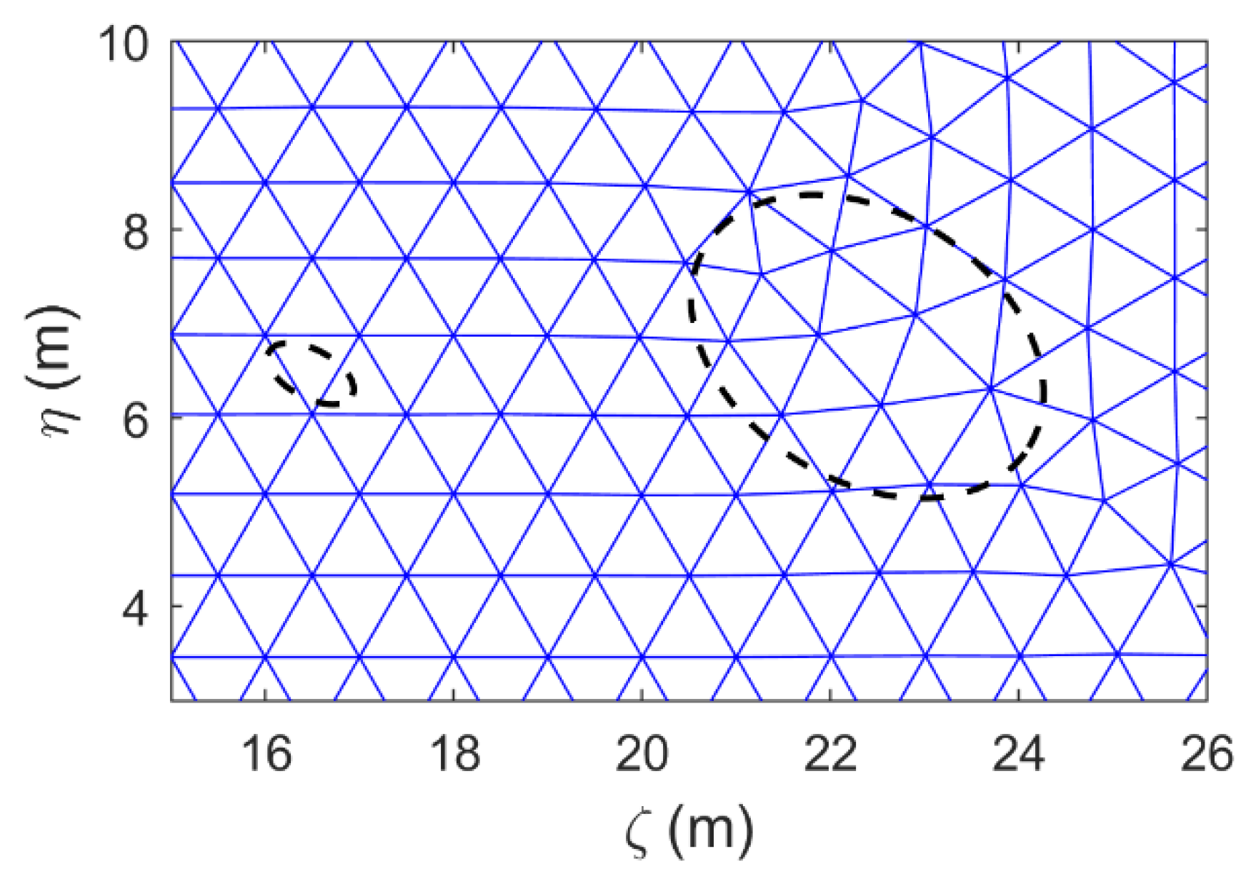
The domain was portioned into unstructured triangular elements with 2447 nodes and 1176 elements, for elements of approximately 1 m, as shown in Figure 2. For the solver options, the absolute, relative, and residual tolerance were set as the default values. The accuracy of the simulation was checked by reducing the relative tolerance, and with simulations with different element sizes (not shown).

3. Results

3.1. Image Processing

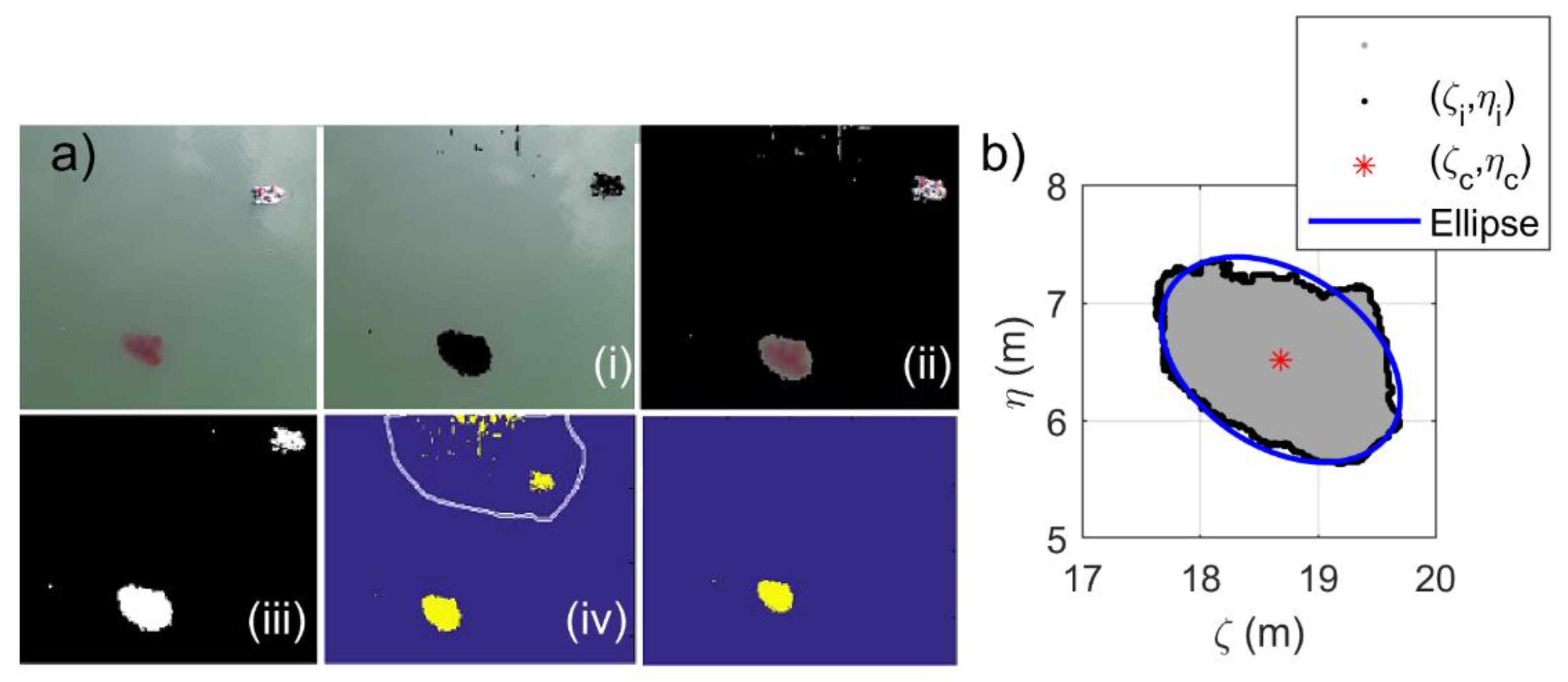
In Figure 3a, the scheme of the image treatment, which consists of the selection of (i) the RGB (red, green, and blue) intensity, (ii) the inverted mask image, (iii) the binary image, and (iv) the selection only of the dye patch, is shown. After georeferencing the image and calculating the geometrical center and the optimal axes, in Figure 3b, the binary image with the boundary dataset of the dye tracer patch, along with the optimal ellipse fit, is shown.

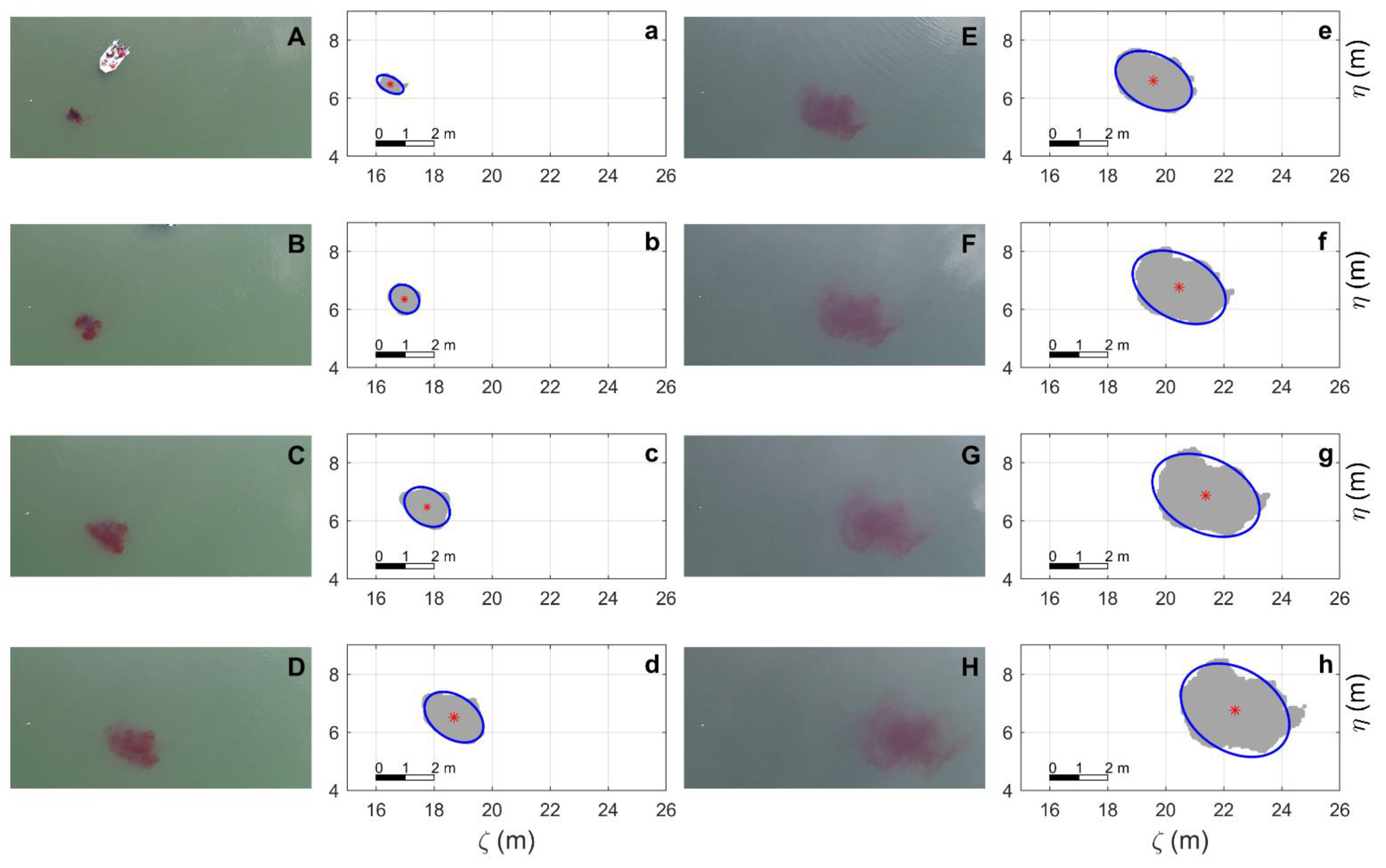
In Figure 4, the main characteristics of the dye patch extent mapping are shown. The images show a dye patch dispersing over time. The first image shows the dye patch after several seconds of release, whereas the last was taken before the patch was not identifiable, due to the reflection of the cloudy sky. The evolution of the corresponding binary image and the optimal ellipse is shown on the right side of Figure 4a–h. It is worth noting that during this experiment (19 July 2018), a light breeze was registered of less than 4 km/h, but enough to displace the boat that was drifting freely with the motor turned off so as to not interfere with the dye patch. Other conditions measured during this experiment were the air temperature of approximately 20 °C, the surface water temperature of 21 °C, and a stratified water column, creating almost ideal conditions to carry out the experiment [40].

3.2. The Velocity Field

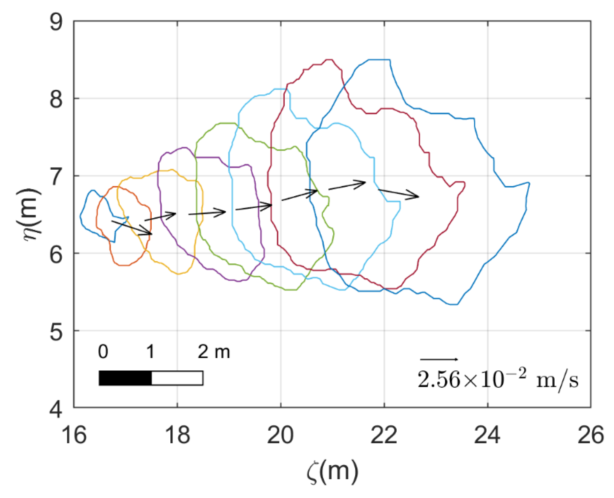
The spatial evolution of the dye patch shows a tendency to the right due to the wind forcing at the site. It was observed that the dye patch was advected ~6 m with an almost homogeneous dispersion of approximately 1 to 5 m of extension for 290 s. The positions of the geometrical center at each time are shown in

Table 1. Data of time and the geometrical center between each contour.

$\mathit{t} \left(s\right)$	${\mathit{\zeta }}_{\mathit{c}}$	${\mathit{\eta }}_{\mathit{c}}$	$\mathit{u} \left(m/s\right)$	$\mathit{v} \left(m/s\right)$
30	16.4837	6.4725	0.0250	−0.0055
50	16.9838	6.3624	0.0194	0.0029
90	17.7586	6.4793	0.0231	0.0011
130	18.6824	6.5220	0.0225	0.0020
170	19.5822	6.6005	0.0220	0.0041
210	20.4634	6.7630	0.0231	0.0030
250	21.3856	6.8815	0.0251	−0.0030

. From the comparison of two consecutive patch contours, the velocity data were obtained according to Equation (14); see Figure 5.

The average velocity for each component used in the transport equation results in the following:

$$U=2.0\times {10}^{-2} \mathrm{m}/\mathrm{s}, V=6.6\times {10}^{-4} \mathrm{m}/\mathrm{s}.$$

(16)

3.3. The Direct and Inverse Problem of the Transport Equation

3.3.1. General Aspects

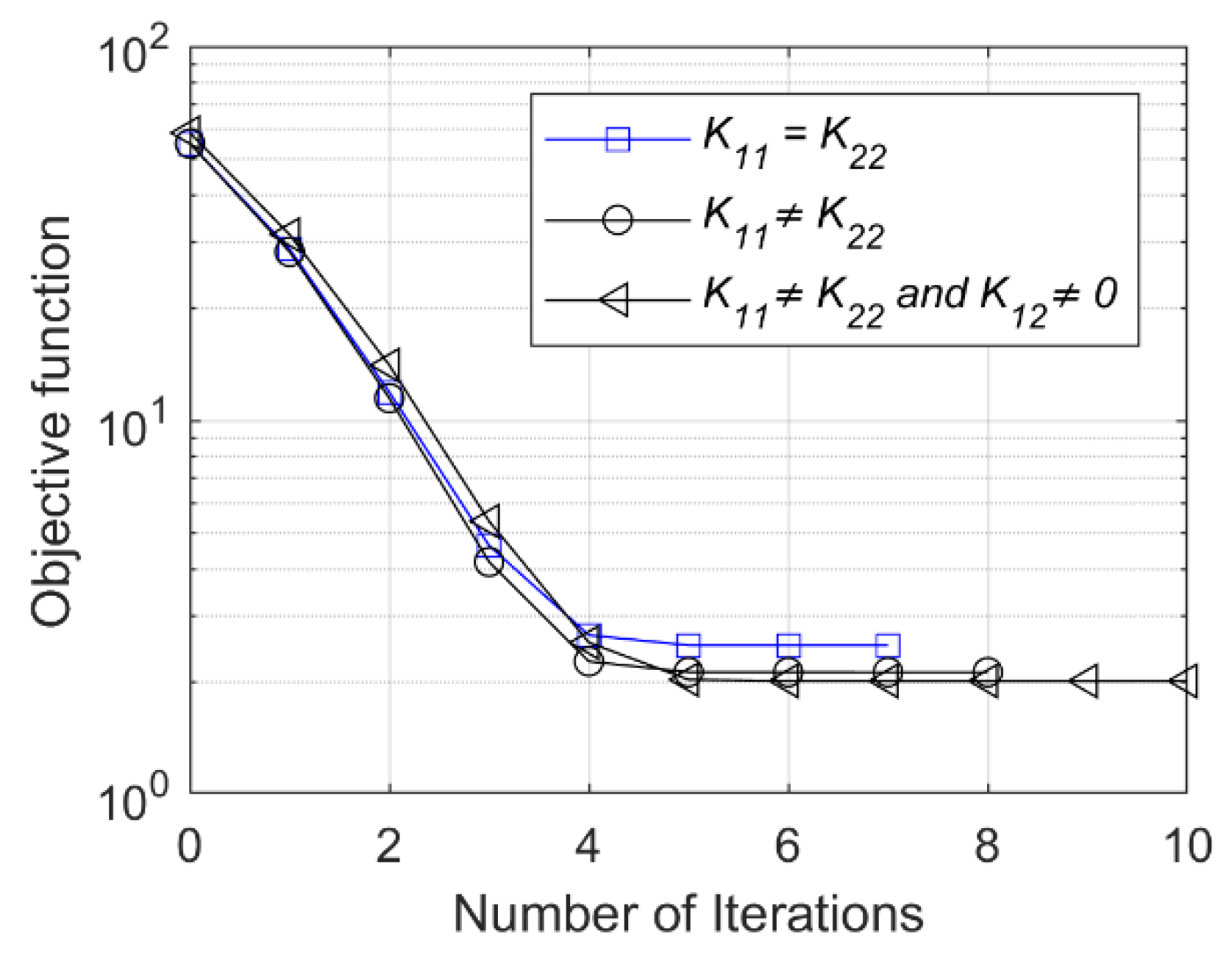
The primary goal of the inverse problem modeling approach is to determine the parameter values that yield the best fit to the observed data. In Figure 6, the objective function $f\left(K\right)$ of Equation (1) and the number of iterations are presented. A smooth convergence is shown, in which the minimization process is completed with a prescribed tolerance of $tol=1\times {10}^{-6}$.

From the analyzed cases, it was indicated that, when $K_{11}\ne K_{22}$ (

Table 2. Parameters and estimation of the diffusion coefficient.

${\mathbf{C}}_{\mathbf{e}}$	${\mathit{K}}_{11}={\mathit{K}}_{22}$	${\mathit{K}}_{11}\ne {\mathit{K}}_{22}$ ${\mathit{K}}_{12}={\mathit{K}}_{21}=0$	${\mathit{K}}_{11}\ne {\mathit{K}}_{22} \mathbf{and}$ ${\mathit{K}}_{12}={\mathit{K}}_{21}\ne 0$
Number of iterations	7	8	10
Number of objective function evaluations	16	27	44
Computational time (s)	~52	~79	~124
$K_{11}$ and $K_{22}$ (${\mathrm{m}}^2/\mathrm{s}$)	0.0032	$K_{11}=0.0051$ $K_{22}=0.0020$	$K_{11}=0.0053$ $K_{22}=0.0021$ $K_{12}=0.0008$
RMSE	0.031	0.029	0.028

), the computational time was greater and the number of iterations was 1 or 3 times higher, but the solution was more precise as the error decreased. When $K_{11}=K_{22}$, the solution was obtained after seven iterations. Additionally, when the anisotropic terms were considered, when $K_{11}\ne K_{22}$ and $K_{12}=K_{21}=0$, the convergence was achieved after eight iterations, and when $K_{11}\ne K_{22}$ and $K_{12}=K_{21}\ne 0$, the optimal solution was obtained after ten iterations.

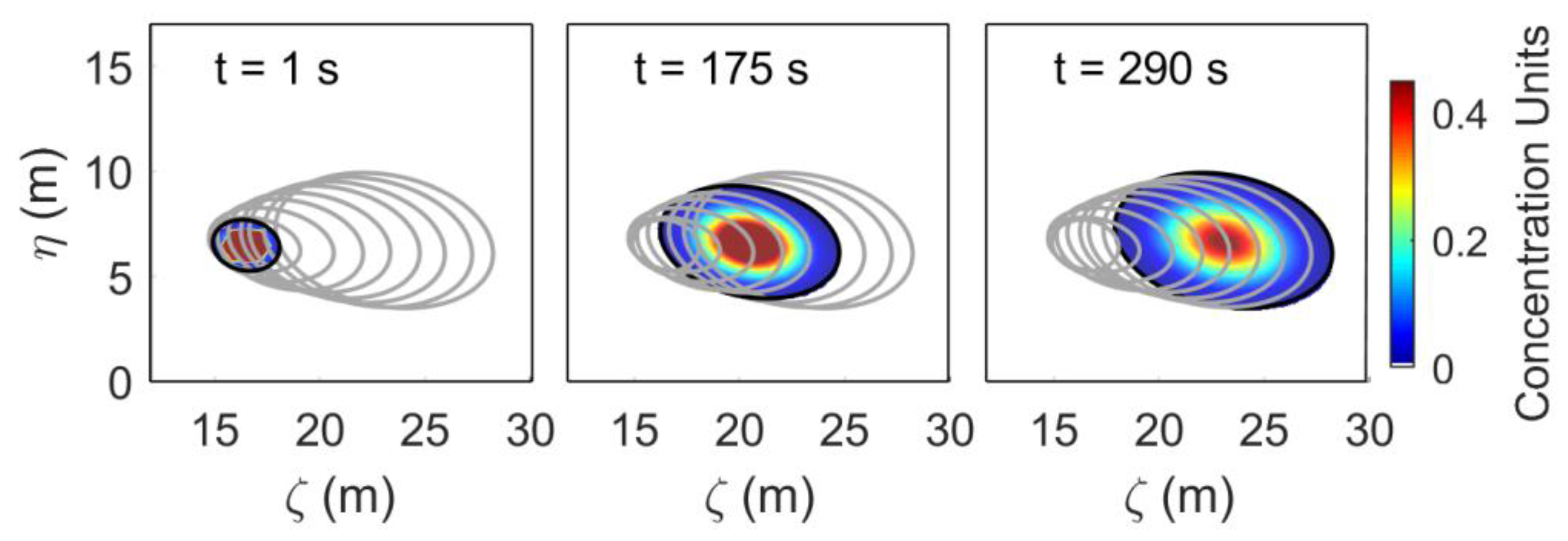
In Figure 7, the time evolution of the case when $K_{11}\ne K_{22}$ and $K_{12}=K_{21}=0$ is shown as an example; the image corresponds to the direct problem for the optimal diffusion coefficients found. It is shown that the evolution of the concentration moved to the right due to the given velocity field, and as time progressed, a lower concentration was observed in the center.

3.3.2. The Final Concentration Snapshots

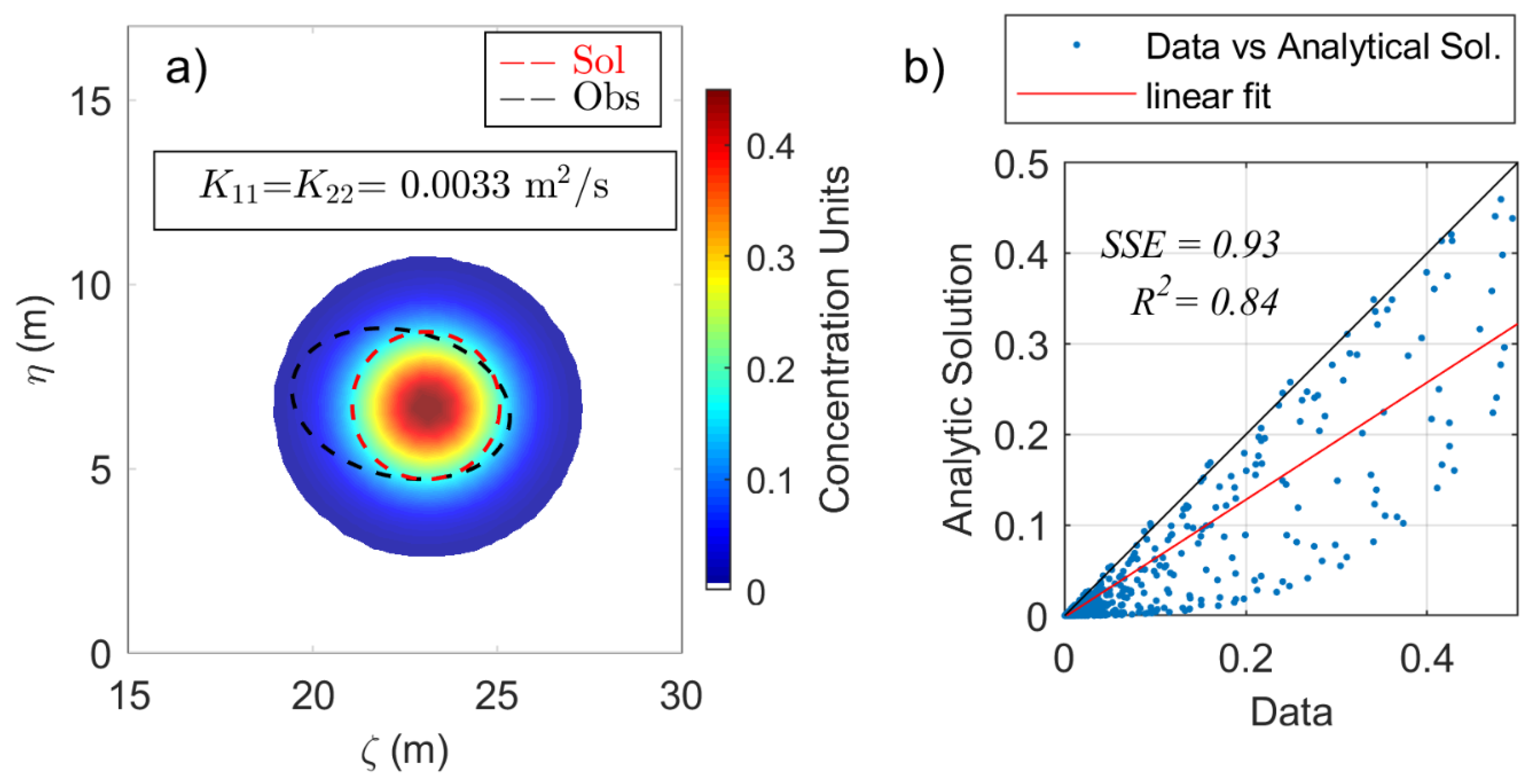
The distribution of the concentration for the final step solution from the simulation is shown in Figure 8a in color contours. In order to obtain a simpler visual analysis, one arbitrary contour is displayed by a black line for the observations and by a red line for the numerical solution of the transport equation once the optimal coefficient was found.

The distribution of the concentration when $K_{11}=K_{22}$ had a circular shape (as expected) and moved slightly to the right with respect to the center of the observations (the ellipse) (Figure 8a). The optimal diffusion coefficients in this case were $K_{11}=K_{22}\approx 0.003 {\mathrm{m}}^2/\mathrm{s}$.

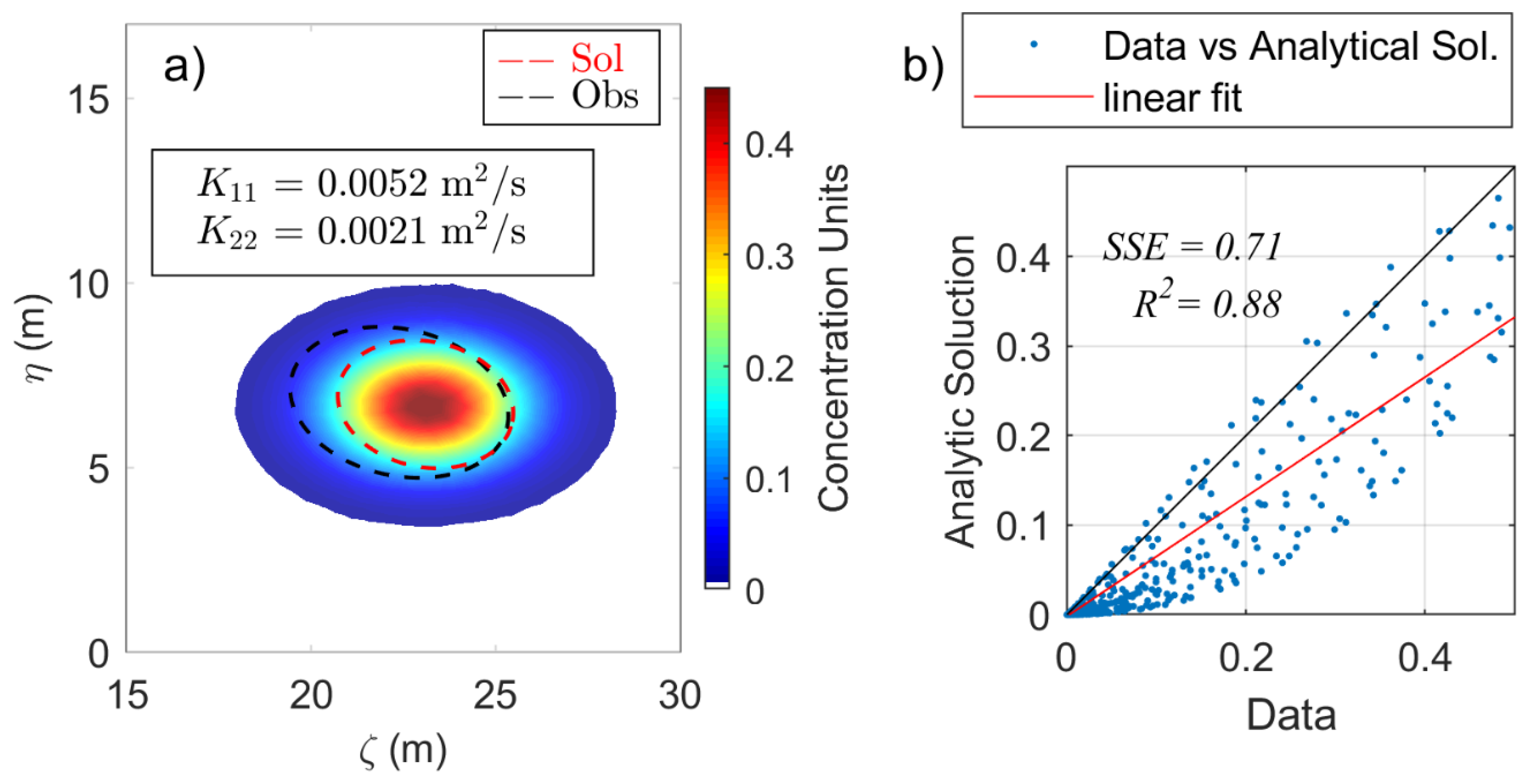
When $K_{11}\ne K_{22}$ and $K_{12}=K_{21}=0$, the solution improved as the resulting numerical shape was an ellipse similar to the one proposed in the observations (Figure 9a), but slightly shifted to the right.

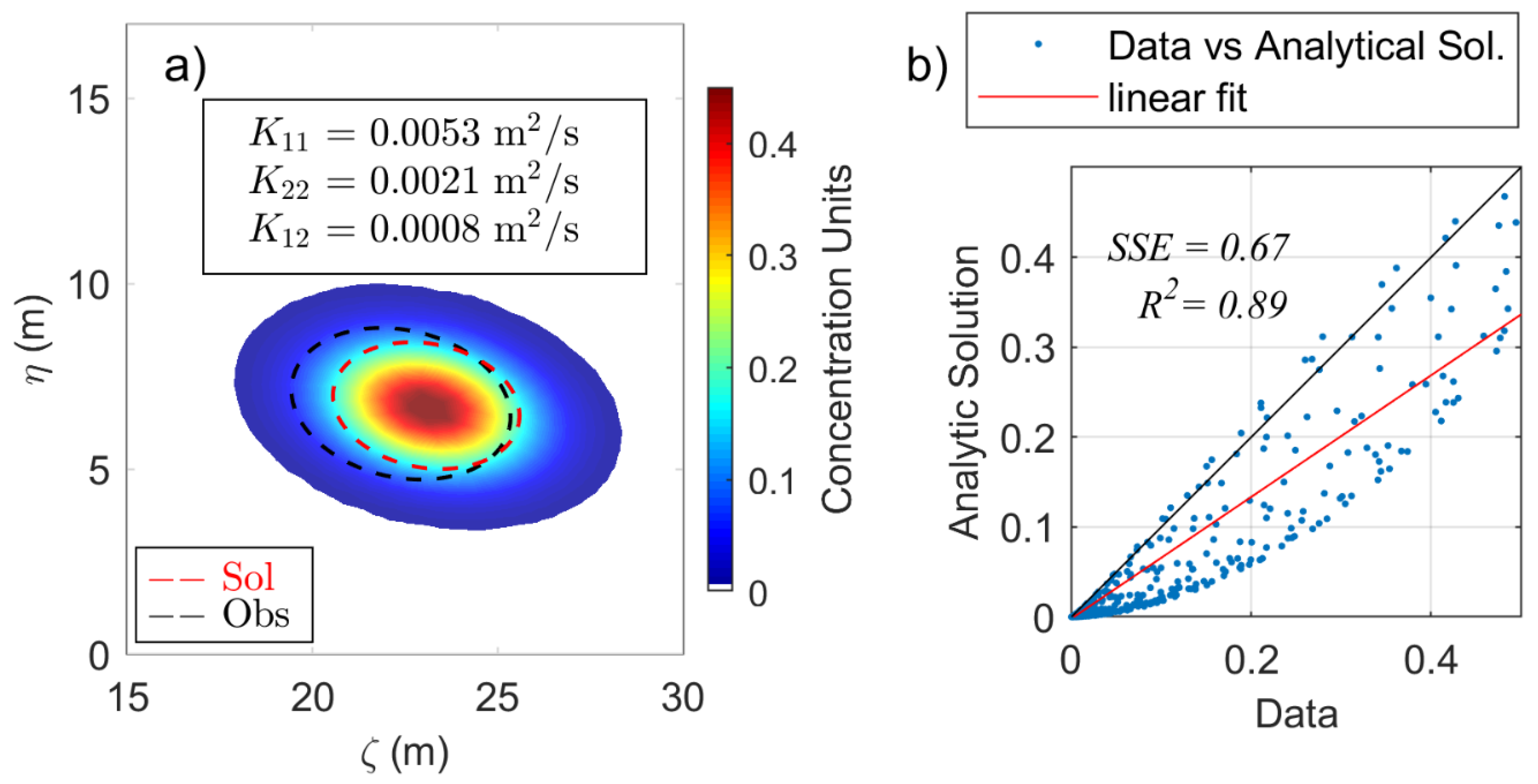
Additionally, in Figure 10a, when $K_{11}\ne K_{22}$ and $K_{12}=K_{21}\ne 0$, a major improvement was achieved as the solution had an ellipse shape, and the orientation matched with the observations; however, a slight shift to the right was still presented.

In Figure 8b, Figure 9b, and Figure 10b, the error between the data and the fit, characterized by the sum of square errors (SSE) and the determination coefficient ($R^2$), is shown. In Figure 8b, SSE = 0.93 and $R^2$ = 084; meanwhile, in Figure 9b, the values correspond to SSE = 0.71 and $R^2$ = 0.88, and in Figure 10b, SSE = 0.67 and $R^2$ = 0.89. Then, the best result was quantitatively obtained for the case when $K_{11}\ne K_{22}$ and $K_{12}=K_{21}\ne 0$, as $R^2$ was closer to unity, and the error tended to zero ($R^2\to 1$ y $SSE\to 0$).

4. Discussion

Based on the results of the diffusion coefficients, the value for these parameters in the study area can be significantly bounded, which is crucial for the forward and inverse problems, as in several studies, the considered values are in the range between 0.0001 and 1 m²/s, and such a wide range can be reflected in significant changes in the dynamics of the transport phenomena. For example, studies [41,42,43,44,45] have been carried out where the distribution of pollutants in lakes and ponds is analyzed using numerical models that solve the advection–diffusion equation, and different values for the diffusion coefficient are considered that span several orders of magnitude (see

Table 3. Studies with different values for the diffusion coefficients considered.

References	Diffusion Coefficient
Kusuma et al. (2017)	$K_{11}=1.28\times {10}^{-5}{ \mathrm{m}}^2/\mathrm{s},$ $K_{22}=1.02\times {10}^{-5}{ \mathrm{m}}^2/\mathrm{s}$
Sunarsih et al. (2020)	$K=1.37\times {10}^{-6}{ \mathrm{m}}^2/\mathrm{s}$
Ahmed (2012)	$K_{11}=1{ \mathrm{m}}^2/\mathrm{s}$ $K_{22}=0.01{ \mathrm{m}}^2/\mathrm{s}$
Hutomo et al. (2019)	$K=0.0004{ \mathrm{m}}^2/\mathrm{s}$ $K=0.00012{ \mathrm{m}}^2/\mathrm{s}$ $K=0.00028{ \mathrm{m}}^2/\mathrm{s}$
Lima et al. (2015)	$K=0.09{ \mathrm{m}}^2/\mathrm{s}$

).

It should be noted that in some of these studies, information was obtained from data of the velocity field, as well as the concentration of different substances measured with very sophisticated instruments, and in several studies, they considered that the propagation rate is proportional to the concentration gradient to estimate the diffusion coefficient.

In the present study, it should be noted that a more dynamic approach was used in which the transport equation itself was basically used to determine its corresponding and more adequate value for a set of observations based on an inverse problem approach.

5. Conclusions

From the dye tracer images, it was noticed that the shape of the distribution of the tracer was not uniform, but for numerical purposes, the ellipse resulted in an improved and accurate approximation; as the typical consideration was a circular shape, although showing similar results, the ellipse was better. Additionally, a perfect match with the ellipse approximation was not expected, as there would be more physical factors to consider in reality, for example, if there was no wind, the diffusion of a point source in a uniform medium should be perfectly circular; however, there are other physical mechanisms that make the diffusion parameter variable according to the conditions such as turbulence, enhanced by waves and its secondary circulations (e.g., Stokes drift and Langmuir circulations). Other factors that could be considered are the chemical or biological properties in the waterbody; however, with further development and measurements, this work can be improved.

Nonetheless, the result of the simulations when $K_{11}=K_{22}$ was $K\approx 0.003{ \mathrm{m}}^2/\mathrm{s}$, whereas, when nonequal coefficients were considered, $K_{11}\ne K_{22}$, $K_{11}\approx 0.005 {\mathrm{m}}^2/\mathrm{s}$, and $K_{22}\approx 0.002 {\mathrm{m}}^2/\mathrm{s}$ were found. The value of the coefficients showed no significant changes, regardless of whether the term $K_{12}$ $\left(=K_{21}\right)$ was considered; however, this parameter was important as it influences the orientation of the ellipse.

Counting with measurements is of great importance as the results of different studies have indicated that pollutants move with the flow and diffuse over time. However, sometimes, the resources are not available to carry out these measurements, hence the importance of this study in terms of the sampling technique and the parameter estimation, which were relatively simple to use. In addition, the values obtained in this paper contribute to a better understanding of the transport phenomena in Lake Zirahuén, which have not been extensively analyzed to date.

Even though the aim was to have a practical implementation to find and bound the values for the diffusion coefficients, the next step could be to consider a bidimensional and space-variable velocity field, solving the transport equation, and applying other numerical scheme solvers or more sophisticated hydrodynamical models, as one of the limitations that arise when implementing the PDE Toolbox is that it only allows the configuration of an analytical velocity field.

Future studies will focus on calibrating a numerical model by using the optimal coefficients calculated in this study. Velocities and diffusion coefficients calculated at different times will serve as a validation.

References

- Janssen, A.B.; Janse, J.H.; Beusen, A.H.; Chang, M.; Harrison, J.A.; Huttunen, I.; Kong, X.; Rost, J.; Teurlincx, S.; Troost, T.A.; et al. How to Model Algal Blooms in Any Lake on Earth. Curr. Opin. Environ. Sustain. 2019, 36, 1–10. [Google Scholar] [CrossRef]
- Mao, J.; Jiang, D.; Dai, H. Spatial–Temporal Hydrodynamic and Algal Bloom Modelling Analysis of a Reservoir Tributary Embayment. J. Hydrog. Environ. Res. 2015, 9, 200–215. [Google Scholar] [CrossRef]
- Boyd, C. Water Quality: An Introduction; Springer: Berlin/Heidelberg, Germany, 2015. [Google Scholar] [CrossRef]
- Wetzel, R. Limnology: Lake and River Ecosystems; Academic Press: Cambridge, MA, USA, 2001; Volume 37. [Google Scholar]
- Ahuja, S. Comprehensive Water Quality and Purification; Elsevier: Amsterdam, The Netherlands, 2014; Volume 1. [Google Scholar] [CrossRef]
- Bachman, S.; Fox-Kemper, B.; Bryan, F. A Diagnosis of Anisotropic Eddy Diffusion from a High-Resolution Global Ocean Model. J. Adv. Model. Earth Syst. 2020, 12. [Google Scholar] [CrossRef] [Green Version]
- Edwards, M. Cross Flow Tensors and Finite Volume Approximation with by Deferred Correction. Comput. Methods Appl. Mech. Eng. 1998, 151, 143–161. [Google Scholar] [CrossRef]
- Qian, Q.; Clark, J.; Voller, V.; Stefan, H. Depth-Dependent Dispersion Coefficient for Modeling of Vertical Solute Exchange in a Lake Bed under Surface Waves. J. Hydraul. Eng. 2009, 135, 187–197. [Google Scholar] [CrossRef]
- Starosolszky, Ö. Lake Hydraulics. Hydrol. Sci. Bull. 1974, 19, 99–114. [Google Scholar] [CrossRef] [Green Version]
- Hundsdorfer, W.; Verwer, J. Numerical Solution of Time-Dependent Advection-Diffusion-Reaction Equations; Springer Series in Computational Mathematics; Springer: Berlin/Heidelberg, Germany, 2003. [Google Scholar] [CrossRef]
- Hasanoğlu, A.H.; Romanov, V.G. Introduction to Inverse Problems for Differential Equations; Springer: Berlin/Heidelberg, Germany, 2017. [Google Scholar] [CrossRef]
- Hurdowar-Castro, H.; Tsanis, I.K. Using Inverse Modeling to Estimate Parameter Values for Three Dimensional Transport of Contaminants in Lake Ontario. Glob. NEST J. 2014, 16, 124–135. [Google Scholar] [CrossRef]
- Domínguez-Mota, F.; Lucas-Martínez, J.S.; Tinoco-Guerrero, G. A Generalized Finite-Differences Scheme Used in Modeling of a Direct and an Inverse Problem of Advection-Diffusion. Int. J. Appl. Math. 2020, 33, 599. [Google Scholar] [CrossRef]
- Hussein, M.; Lesnic, D.; Ismailov, M. An Inverse Problem of Finding the Time-Dependent Diffusion Coefficient from an Integral Condition. Math. Methods Appl. Sci. 2016, 39, 963–980. [Google Scholar] [CrossRef] [Green Version]
- Kamimura, Y. An Inverse Problem in Advection-Diffusion. J. Phys. Conf. Ser. 2007, 73. [Google Scholar] [CrossRef]
- Li, D.S. Convection-Diffusion Modelling for Chemical Pollutant Dispersion in the Joint of Artificial Lake Using Finite Element Method. Bulg. Chem. Commun. 2015, 47, 949–958. [Google Scholar]
- Pecly, J.; Roldão, J. Dye Tracers as a Tool for Outfall Studies: Dilution Measurement Approach. Water Sci. Technol. 2013, 67, 1564–1573. [Google Scholar] [CrossRef]
- Powers, C.; Hanlon, R.; Schmale, D. Tracking of a Fluorescent Dye in a Freshwater Lake with an Unmanned Surface Vehicle and an Unmanned Aircraft System. Remote Sens. 2018, 10, 81. [Google Scholar] [CrossRef] [Green Version]
- Rismal, M.; Kompare, B.; Rajar, R. Contribution of Hydrodynamic and Limnological Modelling to the Sanitation of Lake Bled. In Proceedings of the International Conference on Water Pollution, Bled, Slovenia, 18–20 June 1997. [Google Scholar]
- Clark, D.; Lenain, L.; Feddersen, F.; Boss, E.; Guza, R. Aerial Imaging of Fluorescent Dye in the near Shore. J. Atmos. Ocean. Technol. 2014, 31, 1410–1421. [Google Scholar] [CrossRef] [Green Version]
- Pinton, D.; Canestrelli, A.; Fantuzzi, L. A UAV-Based Dye-Tracking Technique to Measure Surface Velocities over Tidal Channels and Salt Marshes. J. Mar. Sci. Eng. 2020, 8, 364. [Google Scholar] [CrossRef]
- Prasad, D.; Quek, C.; Leung, M. A Precise Ellipse Fitting Method for Noisy Data. In Proceedings of the International Conference Image Analysis and Recognition, Aveiro, Portugal, 25–27 June 2012; Volume 7324. [Google Scholar] [CrossRef]
- Chaudhuri, D. A Simple Least Squares Method for Fitting of Ellipses and Circles Depends on Border Points of a Two-Tone Image and Their 3-D Extensions. Pattern Recognit. Lett. 2010, 31, 818–829. [Google Scholar] [CrossRef]
- Croaze, A.; Pittman, L.; Reynolds, W. Solving Nonlinear Least-Squares Problems with the Gauss-Newton and Levenberg-Marquardt Methods. Available online: https://www.math.lsu.edu/system/files/MunozGroup1%20-%20Paper.pdf (accessed on 11 November 2020).
- Gavin, H. The Levenburg-Marqurdt Algorithm for Nonlinear Least Squares Curve-Fitting Problems. Duke University. Available online: https://people.duke.edu/~hpgavin/ce281/lm.pdf (accessed on 11 November 2020).
- Gill, P.; Murray, W. Algorithms for the Solution of the Nonlinear Least-Squares Problem. Siam J. Numer. Anal. 1978, 15, 977–992. [Google Scholar] [CrossRef]
- Lourakis, M. A Brief Description of the Levenberg-Marquardt Algorithm Implemened by Levmar. Available online: https://www.researchgate.net/publication/239328019_A_Brief_Description_of_the_Levenberg-Marquardt_Algorithm_Implemened_by_levmar (accessed on 11 November 2020).
- Nocedal, J.; Wright, S. Numerical Optimization, Series in Operations Research and Financial Engineering; Springer: New York, NY, USA, 2006. [Google Scholar] [CrossRef] [Green Version]
- Thomson, R.E.; Emery, W.J. Data Analysis Methods in Physical Oceanography, 3rd ed.; Elsevier Science: Amsterdam, The Netherlands, 2014. [Google Scholar]
- Peeters, F.; Hofmann, H. Length-Scale Dependence of Horizontal Dispersion in the Surface Water of Lakes. Limnol. Oceanogr. 2015, 60, 1917–1934. [Google Scholar] [CrossRef] [Green Version]
- Chavent, G. Nonlinear Least Squares for Inverse Problems; Springer: Berlin/Heidelberg, Germany, 2010; Volume 2009. [Google Scholar] [CrossRef] [Green Version]
- Isakov, V. Inverse Problems for Partial Differential Equations; Springer International Publishing: Berlin/Heidelberg, Germany, 2017; Volume 127. [Google Scholar] [CrossRef]
- Kirsch, A. An Introduction to the Mathematical Theory of Inverse Problems; Springer: New York, NY, USA, 2011; Volume 120. [Google Scholar] [CrossRef]
- Byrd, R.; Schnabel, R.; Shultz, G. Approximate Solution of the Trust Region Problem by Minimization over Two-Dimensional Subspaces. Math. Program. 1988, 40, 247–263. [Google Scholar] [CrossRef]
- MATLAB. Matlab Optimization Toolbox. User’s Guide. Available online: https://www.mathworks.com/help/pdf_doc/optim/optim.pdf (accessed on 11 November 2020).
- Coleman, T.; Li, Y. On the Convergence of Interior-Reflective Newton Methods for Nonlinear Minimization Subject to Bounds. Math. Program. 1994, 67, 189–224. [Google Scholar] [CrossRef]
- Moré, J. The Levenberg-Marquardt Algorithm: Implementation and Theory. Numer. Anal. 1978, 630, 105–116. [Google Scholar] [CrossRef] [Green Version]
- Coleman, T.; Li, Y. An Interior Trust Region Approach for Nonlinear Minimization Subject to Bounds. Siam J. Optim. 1996, 6, 418–445. [Google Scholar] [CrossRef] [Green Version]
- Guerrero, M.; Lamberti, A. Cloud Image Processing for Velocity Acquisition. In Proceedings of the Congress International Association for Hydraulic Research, Venice, Italy, 1–6 July 2007; Available online: https://www.researchgate.net/publication/249335362_Cloud_Image_Processing_for_velocity_acquisition (accessed on 11 November 2020).
- Gasca-Ortiz, T.; Pantoja, D.A.; Filonov, A.; Domínguez-Mota, F.; Alcocer, J. Numerical and Observational Analysis of the Hydro-Dynamical Variability in a Small Lake: The Case of Lake Zirahuén, México. Water 2020, 12, 1658. [Google Scholar] [CrossRef]
- Kusuma, J.; Ribal, A.; Mahie, A.G.; Aris, N. On Pollution Distribution on Unhas Lake Using Two Dimension Advection-Diffusion Equation. Far East J. Math. Sci. 2017, 101, 1721–1729. [Google Scholar] [CrossRef]
- Sunarsih, S.; Purwantoro Sasongko, D.; Sutrisno, S.; Agnes Putri, G.; Hadiyanto, H. Analysis of Wastewater Facultative Pond Using Advection-Diffusion Model Based on Explicit Finite Difference Method. Environ. Eng. Res. 2020, 26, 190496. [Google Scholar] [CrossRef]
- Ahmed, S. A Numerical Algorithm for Solving Advection-Diffusion Equation with Constant and Variable Coefficients. Open Numer. Methods J. 2012, 4, 1–7. [Google Scholar] [CrossRef] [Green Version]
- Hutomo, G.; Kusuma, J.; Ribal, A.; Mahie, A.; Aris, N. Numerical Solution of 2-d Advection-Diffusion Equation with Variable Coefficient Using Du-Fort Frankel Method. J. Phys. 2019, 1180. [Google Scholar] [CrossRef]
- Lima, R.; Mesquita, A.; Blanco, C.; Santos, M.; Secretan, Y. An Analysis of Total Phosphorus Dispersion in Lake Used as a Municipal Water Supply. Acad. Bras. Cienc. 2015, 87, 1505–1518. [Google Scholar] [CrossRef] [Green Version]
Figure 1.
Flowchart of the proposed methodology to find the optimal coefficient.
Figure 2.
Rectangular domain with an element size of 1 m. Black ellipses indicate the initial/final condition.
Figure 3.
(a) Image processing steps (i) selection of the RGB intensity, (ii) inverted mask, (iii) binary image, and (iv) selection of the dye patch. (b) Optimal ellipse for the boundary dataset .
Figure 4.
Dye patch extent mapping where the spatial and temporal variation is shown. The images (A–H) show the dye patch dispersing over time, whereas the evolution of the corresponding ellipses after processing is shown in (a–h). The optimal ellipses are shown in blue with the geometrical center marked with a red asterisk.
Figure 5.
Selected dye contours for velocity field computation, and the computed velocities for each contour. The length scale and the velocity scale are shown in the lower part of the figure.
Figure 6.
Objective function and number of iterations, with and .
Figure 7.
Concentration distribution. Concentration contours obtained with the optimal diffusion coefficient and . The gray contour exemplifies the temporal evolution.
Figure 8.
(a) Concentration contours obtained with optimal diffusion coefficients for . Observations are shown in black and the solution in red. In (b), the dispersion diagram of the data and the analytical solution with SSE and is shown.
Figure 9.
Figure 10.
(a) Concentration contours obtained with optimal diffusion coefficients for and . Observations are shown in black and the solution in red. In (b), the dispersion diagram of the data and the analytical solution with SSE and is shown.