
Three Solutions for a Partial Discrete Dirichlet Problem Involving the Mean Curvature Operator


Abstract
:1. Introduction
- for all ;Furthermore, assume that there are , such that
- ;
- .
2. Preliminaries
3. Main Results
- (A1)
- ;
- (A2)
- .
- ;
- .
- ;
- .
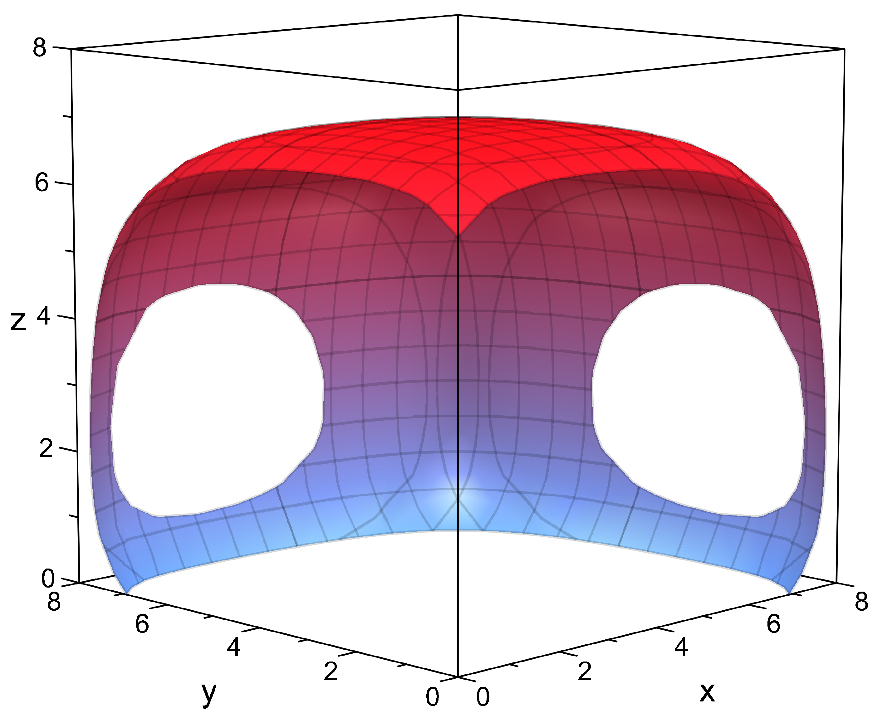
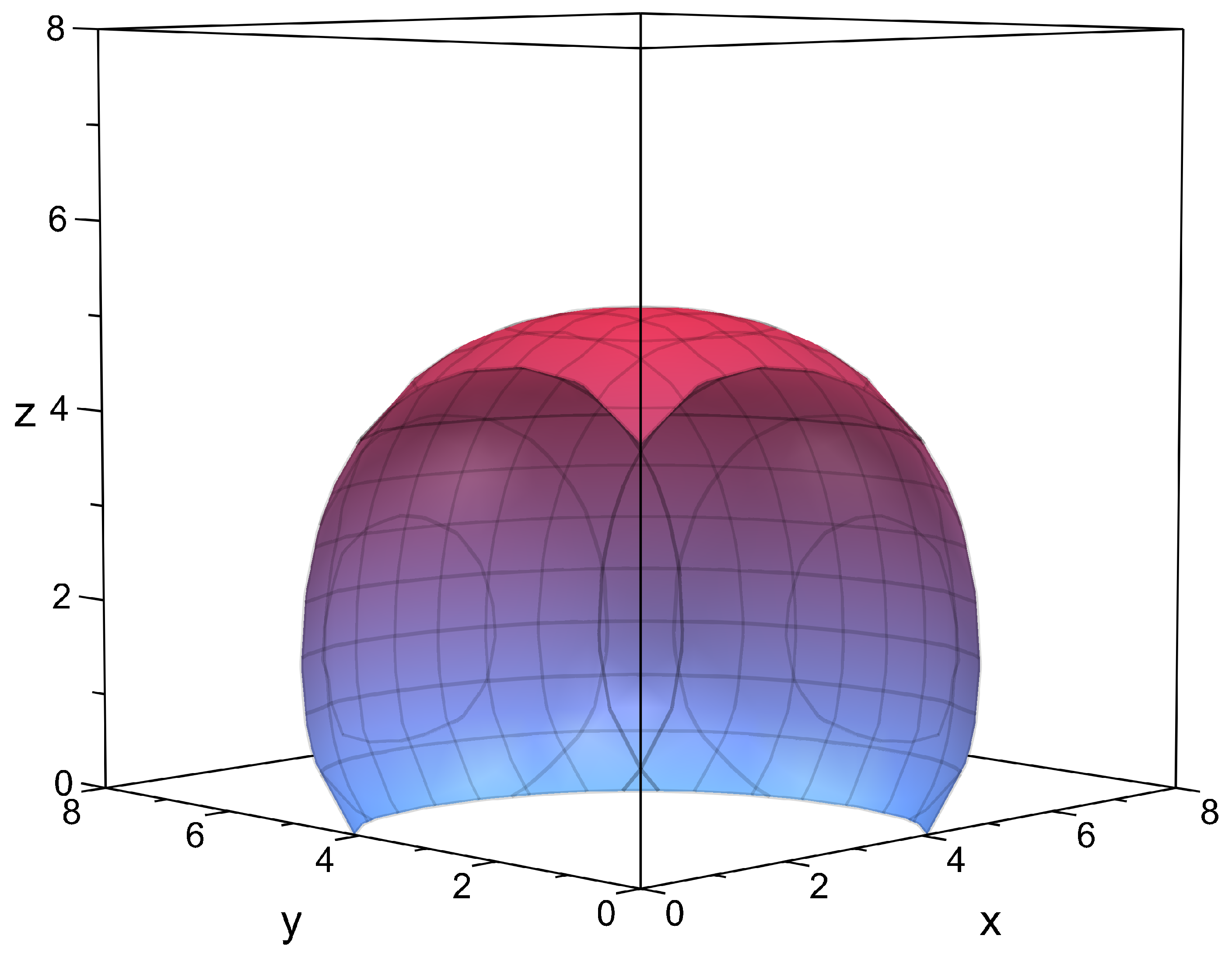
4. Examples
5. Conclusions
Author Contributions
Funding
Institutional Review Board Statement
Informed Consent Statement
Data Availability Statement
Conflicts of Interest
References
- Mawhin, J. Periodic solutions of second order nonlinear difference systems with ϕ-Laplacian: A variational approach. Nonlinear Anal. 2012, 75, 4672–4687. [Google Scholar] [CrossRef]
- Agarwal, R.P. Difference Equations and Inequalities: Theory, Methods and Applications; Marcel Dekker: New York, NY, USA, 1992. [Google Scholar]
- Elaydi, S. An Introduction to Difference Equations, 3rd ed.; Springer Science & Business Media: New York, NY, USA, 2005. [Google Scholar]
- Yu, J.S.; Zheng, B. Modeling Wolbachia infection in mosquito population via discrete dynamical models. J. Differ. Equ. Appl. 2019, 25, 1549–1567. [Google Scholar] [CrossRef]
- Long, Y.H.; Wang, L. Global dynamics of a delayed two-patch discrete SIR disease model. Commun. Nonlinear Sci. Numer. Simul. 2020, 83, 105117. [Google Scholar] [CrossRef]
- Jiang, L.Q.; Zhou, Z. Three solutions to Dirichlet boundary value problems for p-Laplacian difference equations. Adv. Differ. Equ. 2008, 2008, 345916. [Google Scholar] [CrossRef] [Green Version]
- Zhou, Z.; Ling, J.X. Infinitely many positive solutions for a discrete two point nonlinear boundary value problem with ϕc-Laplacian. Appl. Math. Lett. 2019, 91, 28–34. [Google Scholar] [CrossRef]
- Ling, J.X.; Zhou, Z. Positive solutions of the discrete Dirichlet problem involving the mean curvature operator. Open Math. 2019, 17, 1055–1064. [Google Scholar] [CrossRef]
- Wang, S.H.; Long, Y.H. Multiple solutions of fourth-order functional difference equation with periodic boundary conditions. Appl. Math. Lett. 2020, 104, 106292. [Google Scholar] [CrossRef]
- Long, Y.H. Existence of multiple and sign-changing solutions for a second-order nonlinear functional difference equation with periodic coefficients. J. Differ. Equ. Appl. 2020, 26, 966–986. [Google Scholar] [CrossRef]
- Chen, Y.S.; Zhou, Z. Existence of three solutions for a nonlinear discrete boundary value problem with ϕc-Laplacian. Symmetry 2020, 12, 1839. [Google Scholar] [CrossRef]
- Guo, Z.M.; Yu, J.S. Existence of periodic and subharmonic solutions for second-order superlinear difference equations. Sci. China Ser. A 2003, 46, 506–515. [Google Scholar] [CrossRef] [Green Version]
- Liu, X.; Zhou, T.; Shi, H.P.; Long, Y.H.; Wen, Z.L. Periodic solutions with minimal period for fourth-order nonlinear difference equations. Discrete Dyn. Nat. Soc. 2018, 2018, 4376156. [Google Scholar] [CrossRef]
- Mei, P.; Zhou, Z.; Lin, G.H. Periodic and subharmonic solutions for a 2nth-order ϕc-Laplacian difference equation containing both advances and retardations. Discrete Contin. Dyn. Syst. Ser. S 2019, 12, 2085–2095. [Google Scholar]
- Tollu, D.T. Periodic solutions of a system of nonlinear difference equations with periodic coefficients. J. Math. 2020, 2020, 6636105. [Google Scholar] [CrossRef]
- Sugie, J. Number of positive periodic solutions for first-order nonlinear difference equations with feedback. Appl. Math. Comput. 2021, 391, 125626. [Google Scholar] [CrossRef]
- Zhou, Z.; Yu, J.S.; Chen, Y.M. Homoclinic solutions in periodic difference equations with saturable nonlinearity. Sci. China Math. 2011, 54, 83–93. [Google Scholar] [CrossRef]
- Tang, X.H.; Chen, J. Infinitely many homoclinic orbits for a class of discrete Hamiltonian systems. Adv. Differ. Equ. 2013, 2013, 242. [Google Scholar] [CrossRef] [Green Version]
- Zhou, Z.; Ma, D.F. Multiplicity results of breathers for the discrete nonlinear Schrödinger equations with unbounded potentials. Sci. China Math. 2015, 58, 781–790. [Google Scholar] [CrossRef]
- Lin, G.H.; Zhou, Z. Homoclinic solutions of discrete ϕ-Laplacian equations with mixed nonlinearities. Commun. Pure Appl. Anal. 2018, 17, 1723–1747. [Google Scholar]
- Zhang, Q.Q. Homoclinic orbits for discrete Hamiltonian systems with local super-quadratic conditions. Commun. Pure Appl. Anal. 2019, 18, 425–434. [Google Scholar]
- Chen, S.T.; Tang, X.H.; Yu, J.S. Sign-changing ground state solutions for discrete nonlinear Schrödinger equations. J. Differ. Equ. Appl. 2019, 25, 202–218. [Google Scholar] [CrossRef]
- Lin, G.H.; Zhou, Z.; Yu, J.S. Ground state solutions of discrete asymptotically linear Schrödinger equations with bounded and non-periodic potentials. J. Dyn. Differ. Equ. 2020, 32, 527–555. [Google Scholar] [CrossRef]
- Steglinski, R.; Nockowska-Rosiak, M. Sequences of positive homoclinic solutions to difference equations with variable exponent. Math. Slovaca 2020, 70, 417–430. [Google Scholar] [CrossRef] [Green Version]
- Chen, G.W.; Sun, J.J. Infinitely many homoclinic solutions for sublinear and nonperiodic Schrödinger lattice systems. Bound. Value Probl. 2021, 2021, 6. [Google Scholar] [CrossRef]
- Chen, G.W.; Schechter, M. Multiple homoclinic solutions for discrete Schrödinger equations with perturbed and sublinear terms. Z. Angew. Math. Phys. 2021, 72, 63. [Google Scholar] [CrossRef]
- Cabada, A.; Tersian, S. Existence of heteroclinic solutions for discrete p-Laplacian problems with a parameter. Nonlinear Anal. Real World Appl. 2011, 12, 2429–2434. [Google Scholar] [CrossRef]
- Kuang, J.H.; Guo, Z.M. Heteroclinic solutions for a class of p-Laplacian difference equations with a parameter. Appl. Math. Lett. 2020, 100, 106034. [Google Scholar] [CrossRef]
- Shi, B.E.; Chua, L.O. Resistive grid image filtering: Input/output analysis via the CNN framework. IEEE Trans. Circuits Syst. I 1992, 39, 531–548. [Google Scholar] [CrossRef]
- Cheng, S.S. Partial Difference Equations; Taylor & Francis: London, UK, 2003. [Google Scholar]
- Galewski, M.; Orpel, A. On the existence of solutions for discrete elliptic boundary value problems. Appl. Anal. 2010, 89, 1879–1891. [Google Scholar] [CrossRef]
- Heidarkhani, S.; Imbesi, M. Multiple solutions for partial discrete Dirichlet problems depending on a real parameter. J. Differ. Equ. Appl. 2015, 21, 96–110. [Google Scholar] [CrossRef]
- Imbesi, M.; Bisci, G.M. Discrete elliptic Dirichlet problems and nonlinear algebraic systems. Mediterr. J. Math. 2016, 13, 263–278. [Google Scholar] [CrossRef]
- Ji, J.; Yang, B. Eigenvalue comparisons for boundary value problems of the discrete elliptic equation. Commun. Appl. Anal. 2008, 12, 189–198. [Google Scholar]
- Du, S.J.; Zhou, Z. Multiple solutions for partial discrete Dirichlet problems involving the p-Laplacian. Mathematics 2020, 8, 2030. [Google Scholar] [CrossRef]
- Wang, S.H.; Zhou, Z. Three solutions for a partial discrete Dirichlet boundary value problem with p-Laplacian. Bound. Value Probl. 2021, 2021, 39. [Google Scholar] [CrossRef]
- Clement, P.; Manasevich, R.; Mitidieri, E. On a modified capillary equation. J. Differ. Equ. 1996, 124, 343–358. [Google Scholar] [CrossRef] [Green Version]
- Bereanu, C.; Jebelean, P.; Mawhin, J. Radial solutions for some nonlinear problems involving mean curvature operators in Euclidean and Minkowski spaces. Proc. Am. Math. Soc. 2009, 137, 161–169. [Google Scholar] [CrossRef]
- Du, S.J.; Zhou, Z. On the existence of multiple solutions for a partial discrete Dirichlet boundary value problem with mean curvature operator. Adv. Nonlinear Anal. 2022, 11, 198–211. [Google Scholar] [CrossRef]
- Bonanno, G. A critical points theorem and nonlinear differential problems. J. Glob. Optim. 2004, 28, 249–258. [Google Scholar] [CrossRef]


Publisher’s Note: MDPI stays neutral with regard to jurisdictional claims in published maps and institutional affiliations. |
© 2021 by the authors. Licensee MDPI, Basel, Switzerland. This article is an open access article distributed under the terms and conditions of the Creative Commons Attribution (CC BY) license (https://creativecommons.org/licenses/by/4.0/).
Share and Cite
Wang, S.; Zhou, Z. Three Solutions for a Partial Discrete Dirichlet Problem Involving the Mean Curvature Operator. Mathematics 2021, 9, 1691. https://doi.org/10.3390/math9141691
Wang S, Zhou Z. Three Solutions for a Partial Discrete Dirichlet Problem Involving the Mean Curvature Operator. Mathematics. 2021; 9(14):1691. https://doi.org/10.3390/math9141691
Chicago/Turabian StyleWang, Shaohong, and Zhan Zhou. 2021. "Three Solutions for a Partial Discrete Dirichlet Problem Involving the Mean Curvature Operator" Mathematics 9, no. 14: 1691. https://doi.org/10.3390/math9141691