Testing a Recent DEMATEL-Based Proposal to Simplify the Use of ANP

Abstract

The Analytic Network Process (ANP) is a well-known multi-criteria decision method that allows the relationships between its elements to be incorporated into the model. The large number of questions to be answered is one of the main drawbacks of the method, since it is time consuming for decision makers and experts who participate in the decision process. A recent DEMATEL-based ANP proposal can significantly reduce the number and the complexity of questions. This proposal was simply exposed and lacked an experimental test with real cases. The fundamental objective of this work is to answer the question: Does it work? In this work, this new proposal is applied to 45 ANP cases published in the literature. Variants to the verified proposal have also been identified. The results obtained show that the values of the priorities and the ranks obtained with this new proposal are very similar to the results obtained with the ANP, reducing the number of questions required by 42% on average. Additionally, in this work you can find the compilation of the 45 ANP weighted supermatrices to use in your investigations.

1. Introduction

The Analytic Network Process (ANP) is a generalisation of the Analytic Hierarchy Process (AHP) method, both proposed by Thomas Saaty, used in multi-criteria decision analysis [1,2,3]. The AHP separates the elements of the decision problem into the following two clusters: criteria and alternatives. The criteria are structured using hierarchies. The criteria within the same hierarchical level are prioritised using pairwise comparisons matrices. Pairwise comparison matrices are also used to evaluate (prioritise) the alternatives for the lower-level criteria of the hierarchy.

In the AHP, it is considered that each criterion only influences the hierarchical criterion on which it depends and that the alternatives only influence the criteria of the last hierarchical level. Instead, the ANP considers that the elements of the decision problem, alternatives and criteria, can influence relationships with any other element of the model. Thus, the resulting model is a network or graph, weighted and oriented, allowing an influence or reciprocal relationship between the elements. The ANP includes the AHP, since a hierarchy is a particular case of a network. An ANP model groups the criteria into one or more clusters. If the model includes alternatives, these are usually grouped into a single cluster, although not necessarily. Saaty proposes using pairwise comparison matrices to prioritise the elements of the same cluster that have an influence over an element, and to prioritise the clusters that influence the same cluster.

One of the critiques toward the ANP is that it is too complex to be applied practically [4]. Experts and decision-makers have to invest a lot of time given the greater complexity of the models and the ANP method. It requires the elaboration of extensive questionnaires to identify and weigh the influences between elements and clusters. In addition, there are often questions that are complex for decision makers to understand. The following question is an example: “In order to achieve the goal, compare with respect to A, which is more important/has more influence, A or B?”. This means that many decision-makers end up preferring to work with hierarchical models that are easier to use and understand, although most decision problems must not be structured hierarchically due to the interactions and dependencies of the elements of some levels above the others.

The Decision-Making Trial and Evaluation Laboratory (DEMATEL) method proposed by Fontela and Gabus [5] is another technique used in multi-attribute decision-making that builds a network with the components of the problem. It differs from the ANP in that the relationships are causally dependent, that is, cause and effect relationships are based on surveys to determine the interdependence of direct and indirect relationships or influences between components or variables/attributes and the strength of those relationships. Furthermore, in DEMATEL, decision makers directly assess the influence intensity between components [6].

In recent years, specifically since 2008, the number of publications on joint hybrid mathematical modelling of the DEMATEL and ANP techniques has increased [4]. Using a detailed bibliometric analysis, in [4] these hybrid techniques are classified into the following four main categories: Network Relationship Map (NRM) of ANP, Inner Dependency in ANP, Cluster-Weighted ANP and DEMATEL-Based ANP (DANP). These categories differ in whether they use the ANP or DEMATEL in each of the following stages: Criteria structuring, Inner dependency, Outer dependency and Weighting clusters. DANP uses DEMATEL in all four stages. In [7,8,9], applications with hybrid AHP models with other multicriteria techniques can be consulted.

In this context, Kadoić, Divjak and Begičević Ređep [10] made a modified DANP integration proposal to decrease the complexity of the decision-making process, reduce its duration by reducing the number of questions to be answered by decision makers and experts and increase users’ understanding of the method. This proposal includes two variants of calculation and, in addition, has the following two striking aspects that we have not previously encountered in the literature: (1) to consider all the elements in a single cluster; (2) to use a DEMATEL scale for the intensities of influence in the ANP method.

In [10], the authors simply expose their proposal with simple and partial examples; therefore, this article aims to verify the effectiveness of that proposal using it in real cases, and answer the question “Does it work?” Our objective is to verify how much the results are affected by the reduction in the number of questions (information) that are incorporated into the model, the proposed change of scales, as well as to determine which of the two proposed variants obtains better results. For this, ANP cases published in scientific journals have been identified. After applying the modified DANP proposal to the published weighted matrices, the results of the original model are compared with the results obtained with this new proposal. The decrease in the complexity of the decision-making process is also analysed when using this new proposal. Finally, possible calculation variants are identified, not exposed in the original article.

The structure of the article is as follows: Section 2 summarises the theoretical background of the ANP and DEMATEL methods and of the DANP integration proposal whose applicability is studied. Section 3 presents the method followed to contrast the new proposal. Section 4 presents as an illustrative example of the calculations of one of the cases to which this new proposal has been applied. Section 5 collects the results of all the cases and their respective analysis. Finally, Section 6 presents the conclusions and proposals for future work.

Furthermore, in this work you can find the 45 ANP weighted supermatrices of the published cases to use in your investigations, and all the matrices and results of our work, to ensure that it can be reproduced and verified.

2. Theoretical Background

This section presents the ANP and DEMATEL methods, and the studied new approach with the fundamental steps.

2.1. The ANP Method

Mathematician Thomas L. Saaty proposed, at the end of the 1970’s, a structured method as a solution to specific problems in decision-making, which allows the relative weight of decision criteria to be determined and the alternatives to be prioritised by means of the formalisation of the expert judgment, preferences and perceptions of a multidisciplinary team through the construction of the following three-level structured hierarchy: objective, criteria and alternatives [11]. The AHP method is one of the most used methods [12] and presents favourable results when considering decision problems in which a hierarchical structure of criteria is established and the independence in preference between the criteria can be assumed and verified. It has been successfully applied in practice, as presented by Thomas L. Saaty, through observations and suggestions for planning and execution in group decision-making. However, the AHP has a limitation regarding the interactions and dependencies between the elements in the hierarchy.

To overcome this limitation, Saaty considered the dependencies and the feedback of the elements, developing the ANP method [2]. Saaty indicates that the ANP provides a general framework to deal with decisions without making assumptions about the independence of higher-level elements with respect to lower-level elements, as well as the independence of elements within the same level [13].

The ANP represents any decision-making problem as a network of criteria and alternatives (all called elements), gathered in groups. All the elements of the network can be related in any way possible, which means that a network can incorporate feedback and interdependent relationships within and between groups. This allows working with interdependences between criteria and provides a more precise approach to complex model surroundings. The influence of some elements in the network on other elements in that network can be represented in a supermatrix. This new concept is a two-dimensional element-by-element matrix, which adjusts the relative importance weights in individual pairwise comparison matrices to form a new global supermatrix with the eigenvectors of the adjusted relative importance weights.

The ANP comprises the following main steps:

• Given a decision problem with $x_1, x_2, \dots , x_N$ elements, the first step consists of building a model grouping the elements into $c_1, c_2, \dots , c_G$ clusters.
  Let $x_i^c$ be the $i$ element of the model, which belongs to cluster $c$, with $i=1, \dots , N$, $c=1, \dots , G$.
  Let $x^{c_a}$ be the elements of cluster $c_a$, $\left\{x_i^c : c=c_a\right\}$. Let $n_{C_a}$ be the number of elements of cluster $c_a$.
• Identify the elements’ relationships, ask the DM, and obtain the (N × N) elements’ relationships matrix, $\mathit{R}= \left[r_{i,j}\right] = \left[r_{i,j}^{c_{a,}{c}_b}\right]$. $r_{i,j}^{c_{a,}{c}_b}\in \left\{0,1\right\}$ where $c_a, c_b=1,\dots , G$ and $i,j=1,\dots , N$:
  • $r_{i,j}^{c_a,c_b}=0$ indicates that the element $x_i^{c_a}$ has no influence on the element $x_j^{c_b}$, and in the graphical model there is not an arc from $x_j^{c_a}$ to $x_i^{c_b}$;
  • $r_{i,j}^{c_{a,}{c}_b}=1$ indicates that the element $x_i^{c_a}$ has some influence on the element $x_j^{c_b}$, and in the graphical model there is an arc from $x_j^{c_a}$ to $x_i^{c_b}$.
• Obtain the (G × G) clusters’ relationships matrix, $\widehat{\mathit{R}}=\left[{\widehat{r}}_{c_a,c_b}\right]$. ${\widehat{r}}_{c_a,c_b}=\left\{0,1\right\}$ where $c_a, c_b=1,\dots ,G$.
  • ${\widehat{r}}_{c_a,c_b}=0$ indicates that any element of cluster $c_a$ has influence on any element of cluster $c_b$, as follows:

    $${\widehat{r}}_{c_a,c_b}=0 \to \forall i,j\hspace{1em}i,j=1,\dots ,N : r_{i,j}^{c_{a,}{c}_b}=0$$

    (1)
  • ${\widehat{r}}_{c_a,c_b}=1$ indicates that some element of cluster $c_a$ has influence on some (at least one) elements of cluster $c_b$, as follows:

    $${\widehat{r}}_{c_a,c_b}=1 \to \exists i,j i,j=1,\dots ,N : r_{i,j}^{c_{a,}{c}_b}=1$$

    (2)
• Use pairwise matrices to compare the influence of the elements belonging to each cluster on any element, and derive a priority vector, and obtain the (N × N) Unweighted Supermatrix, $\mathit{U}=\left[u_{i,j}^{c_a,c_b}\right]$, with $u_{i,j}^{c_{a,}{c}_b}\in \left[0,1\right],$ $c_a, c_b=1,\dots ,G$ and $i,j=1,\dots ,N$, where $u_{i,j}^{c_{a,}{c}_b}$ is the influence of element i, which belongs to cluster $c_a$, on element j, which belongs to cluster $c_b$. In the pairwise matrices, as in the AHP, Saaty proposes the use of 1-to-9 ratio scales to rate the decision maker’s preferences, known as Saaty’s Fundamental Scale. The Consistency Ratio (CR) is used to check judgement inconsistencies of the pairwise matrices.
  • $u_{i,j}^{c_{a,}{c}_b}=0$ indicates that element $i$, which belongs to cluster $c_a$, has no influence on element $j$, which belongs to cluster $c_b$, as follows:

    $$u_{i,j}^{c_{a,}{c}_b}=0 ⟷ r_{i,j}^{c_a,c_b}=0$$

    (3)
  • $u_{i,j}^{c_{a,}{c}_b}=1$ indicates that element $i$, which belongs to cluster $c_a$, is the unique element of cluster $c_a$, which has influence on element $j$, which belongs to cluster $c_b$, as follows:

    $$u_{i,j}^{c_{a,}{c}_b}=1 \Rightarrow \forall k\ne i, k=1,\dots ,N :x_k\in x^{c_a}\to r_{k,j}^{c_a,c_b}=0$$

    (4)
  • Given a cluster, $c_a$, and an element, j, that belongs to cluster $c_b$, $x_j^{c_b}$, the sum of the unweighted values of the elements that belong to $c_a$, which have influence on $x_j$, is 1. If no element of $c_a$ has influence on $x_j$, then the sum is 0.
  Given $c_a, x_j^{c_b}$, the following applies:

  $${\displaystyle \sum }_{\begin{array}{c}k=1\\ k : x_k\in x^{c_a}\end{array}}^N\left(u_{k,j}^{c_a,c_b}\right)\in \left\{0,1\right\}$$

  (5)
  Column’s sum, ${{\displaystyle \sum }}_{i=1}^N\left(u_{i,j}\right)$, indicates how many clusters have influence on the column element.
• Conduct pairwise comparisons on the clusters, obtaining $\widehat{\mathit{U}}=\left[{\widehat{u}}_{c_a,c_b}\right]$, the (G × G) cluster weights matrix, with ${\widehat{u}}_{c_a,c_b}\in \left[0,1\right] ,$  $c_a, c_b=1,\dots ,G,$ where ${\widehat{u}}_{c_a,c_b}$ is the influence of cluster $c_a$ on cluster $c_b$.
  • ${\widehat{u}}_{c_a,c_b}=0$, shows that any element of cluster $c_a$ has influence on any element of cluster $c_b$, as follows:

    $${\displaystyle \sum }_{c_a=1}^G\left({\widehat{u}}_{c_a,c_b}\right)=1$$

    (6)
• Calculate $\mathit{W}=\left[w_{i,j}^{c_a,c_b}\right],$ the (N × N) Weighted Supermatrix, with $w_{i,j}^{c_{a,}{c}_b}\in \left[0,1\right],$ $c_a, c_b=1,\dots ,G$ and $i,j=1,\dots ,N$, where $w_{i,j}^{c_{a,}{c}_b}=u_{i,j}^{c_{a,}{c}_b}· {\widehat{u}}_{c_a,c_b}$.
  • $w_{i,j}^{c_{a,}{c}_b}$ is the weighted influence of element i, which belongs to cluster $c_a$, on element j, which belongs to cluster $c_b$, as follows:

    $${\displaystyle \sum }_{i=1}^N\left(w_{i,j}^{c_{a,}{c}_b}\right)\in \left]0,1\right]$$

    (7)
• Calculate $\mathit{Q}=\left[q_{i,j}^{c_a,c_b}\right]$, the (N × N) Normalized and Weighted Supermatrix, with $q_{i,j}^{c_{a,}{c}_b}\in \left[0,1\right],$ $c_a, c_b=1,\dots ,G$ and $i,j=1,\dots ,N$, where $q_{i,j}^{c_{a,}{c}_b}=\frac{w_{i,j}^{c_{a,}{c}_b}}{{{\displaystyle \sum }}_i\left(w_{i,j}^{c_{a,}{c}_b}\right)}$.
  • $q_{i,j}^{c_{a,}{c}_b}$ is the normalized weighted influence of element i, which belongs to cluster $c_a$, on element j, which belongs to cluster $c_b$.
  • ${{\displaystyle \sum }}_i\left(q_{i,j}^{c_{a,}{c}_b}\right)=1$. $\mathit{Q}$ is a left-stochastic matrix.
• Calculate $\mathit{L}=\underset{k\to \infty }{\lim }{\mathit{Q}}^k$, the Limit Supermatrix. $l_i$ is the final priority of element $x_i$. If $x_i$ is an alternative, $l_i$ is the rating of the alternative. If $x_i$ is a criterion, $l_i$ is the weight of the criterion.

2.2. The DEMATEL Method

DEMATEL is a comprehensive method developed by the “Science and Human Affairs Program of the Battelle Memorial Institute of Geneva” between 1972 and 1976, proposed by Fontela and Gabus. It is based on the graph theory to build and analyse structural digraph models of causal relationships between complex factors of a subsystem, to present interdependent relationships and influencing values, thus, improving the understanding of the structural relationship between the elements of the causal groups and the affected group [14].

The procedure to calculate the level of interdependence of the factors considered in the DEMATEL method is the following [5,15]:

• Create expert perception matrixes X¹, X², ..., X^H. Assuming that there are H experts in the observed survey and n factors that are considered, each expert should determine the level of influence of factor i to the factor j. The comparative analysis of a couple of factors i and j by the expert, k, is denoted by $x_{ij}^k$, while i = 1, ..., n; j = 1, ..., n; k = 1, ..., H. The value of each couple $x_{ij}^k$, adopts an integer value with the following meaning: 0—no influence; 1—low influence; 2—medium influence; 3—high influence; 4—very high influence. The answer of the expert, k, is represented by a matrix of rank $n\times n$, while each element k of the matrix in the expression $X^{\mathit{k}}={\left[x_{ij}^k\right]}_{n\times n}$ denotes a non-negative number $x_{ij}^k$, where k =1, ..., H.
• Accordingly, matrixes X¹, X², ..., X^H represent answer matrixes of each of the H experts. The diagonal elements of each expert answer matrix are all set to zero because the factor cannot affect itself.
  Calculate the average perception matrix A. Based on the determined answer matrixes ${\mathit{X}}^k={\left[x_{ij}^k\right]}_{n\times n}$ from all of the H experts, it could be calculated that the average answer matrix, $\mathit{A}={\left[a_{ij}\right]}_{n\times n}$, which represents a medium value of the opinions of all the H respondents (experts) for each element of matrix A, where

  $$a_{ij}=\frac{1}{H}{\displaystyle \sum }_{k=1}^H{x}_{ij}^k$$

  (8)
  Matrix A shows the initial effects caused by a particular factor, but also the initial effects it receives from other factors.
• Calculate the average normalized perception matrix D. The matrix D is calculated from the matrix A, as follows:
  Let

  $$s=max\left(ma{x}_{1\le i\le n}{{\displaystyle \sum }}_{j=1}^n{a}_{ij};ma{x}_{1\le i\le n}{{\displaystyle \sum }}_{i=1}^n{a}_{ij}\right)$$

  (9)
  Then,

  $$\mathit{D}=\mathit{A}/s$$

  (10)
  As the sum of each row i of the matrix A represents the total direct effects that the factor i gives to other factors, the expression $ma{x}_{1\le i\le n}{\displaystyle \sum }_{j=1}^n{a}_{ij}$, represents the most important total direct effects that the specified factor gives to other factors. Similarly, as the sum of each column j of the matrix A represents the total direct effects that the factor j receives from other factors, the expression $ma{x}_{1\le j\le n}{\displaystyle \sum }_{i=1}^n{a}_{ij}$, represents the most important total direct effects that the specified factor receives from other factors. s considers the highest value of the above-mentioned two expressions. Matrix D is obtained when each element a_ij of matrix A is divided by expression s. Each element d_ij of the matrix D takes values between 0 and less than 1.
• Calculate the total relation matrix T. Matrix T is an n × n matrix and it is calculated as follows:

  $$\mathit{T}=\mathit{D}{\left(\mathit{I}-\mathit{D}\right)}^{-1}$$

  (11)

  where I is an $n\times n$ identity matrix.
  Let the sums of the rows and columns of the matrix T be separately represented by vector r and vector c, explicitly as follows:

  $$\mathit{r}={\left[r_{ij}\right]}_{n\times 1}={\left[{\displaystyle \sum }_{j=1}^n{t}_{ij}\right]}_{n\times 1}$$

  (12)

  $$\mathit{c}={\left[c_j\right]}_{n\times 1}^{\prime }={\left[{{\displaystyle \sum }}_{i=1}^n{t}_{ij}\right]}_{1\times n}$$

  (13)

  where symbol ′ stands for a transposed matrix. Let r_i be the sum of the ith row in matrix T. Then, r_i represents the total direct and indirect effects that the factor i has given to other factors. Let c_j represents the sum of the jth column in matrix T. Then, c_j shows the total effects, both direct and indirect, received by a factor j given by other factors. In the case when i = j, then the term (r_i + c_i) represents the degree of importance of the factor, and the term (r_i − c_i) represents the net effect that the factor contributes to the system in relation to other factors. If the term (r_i − c_i) is positive, the factor i is the net causer, and if the previous expression is negative factor i is the net receiver.
• Set a threshold value p and obtain the NRM. The threshold value p is determined on the basis of expert opinion, which filters out the negligible or small effects in the matrix T. The value of the elements of matrix T, which are smaller than or equal to the adopted value p, is set to zero, while other elements of the matrix T, which are larger than the adopted value p, retain their present value. Should the adopted value p be too low, the structure of the system will remain complex and difficult to understand, while if the threshold value p is too high, the structure would be over-simplified and important influences will be ignored. Therefore, based on the adopted threshold value p, we can filter minor effects in matrix T, based on which NRM will be obtained, which facilitates an understanding of the relationships in the considered system.

2.3. The New DANP Proposal

Kadoić et al. [10] propose a new approach in DEMATEL and ANP integration, using two modified techniques that use pre-existing ideas of hybrid models of the two models. The proposal indicates the following stages:

1.

To create a network structure of the decision-making problem using part of the DEMATEL algorithm to establish a matrix of influences between criteria called X. The structure of the network is represented by a weighted graph. That is, the elements’ relationships matrix, R, of the ANP is ignored and instead, matrix X is obtained, as explained in steps one and two of DEMATEL.

2.

To calculate an ANP weighted matrix from the previous X. Although the proposal by Kadoić et al. allows the unweighted and cluster matrix to be calculated, they recommend that observing all the criteria as one big cluster is preferable. With this suggestion, the ANP Weighted Supermatrix is directly obtained. They propose the following two methods to calculate the influences on each column element:

• Applying the normalisation by the sum. Each column in X is divided by the sum of the column. Therefore, a stochastic by column Weighted Supermatrix is directly obtained.
• Using a transition matrix. For each column, a pairwise matrix is computed with the row elements that have influence on each column. The difference between the X values of influence intensity is transformed in Saaty’s judgement scale using a transition matrix. The transition matrix proposed by Kadoić et al. [10] is shown in

  Table 1. Matrix of transition.

  Difference in Terms of Intensity of Influence	Judgement on Saaty’s Scale
  4 (4 − 0)	9
  3 (3 − 0, 4 − 1)	7
  2 (2 − 0, 3 − 1, 4 − 2)	5
  1 (1 − 0, 2 − 1, 3 − 2, 4 − 3)	3
  0 (0 − 0, 1 − 1, 2 − 2, 3 − 3, 4 − 4)	1
  −1 (0 − 1, 1 − 2, 2 − 3, 3 − 4)	1/3
  −2 (0 − 2, 1 − 3, 2 − 4)	1/5
  −3 (0 − 3, 1 − 4)	1/7
  −4 (0 − 4)	1/9

  . The intermediate values are interpolated, for example, when an X average matrix is calculated from several experts. The normalised eigenvector associated with the maximum eigenvalue represents the influence priorities in the weighted matrix column. In a model with several clusters, an influence matrix between the clusters must be obtained according to step one, and the priorities between the clusters must be obtained according to the two methods indicated in point two (normalisation by the sum or transition matrix). The weighted matrix is obtained by multiplying the influence priorities of the elements by the influence priorities of the clusters and normalising when needed. In a model without alternatives, using a single cluster almost guarantees avoiding questions such as “Compare with respect to A, which is more important/has more influence A or B?”.

3.

Calculating the ANP limit matrix. In this last step, the limit matrix is calculated with the global influences following the ANP method.

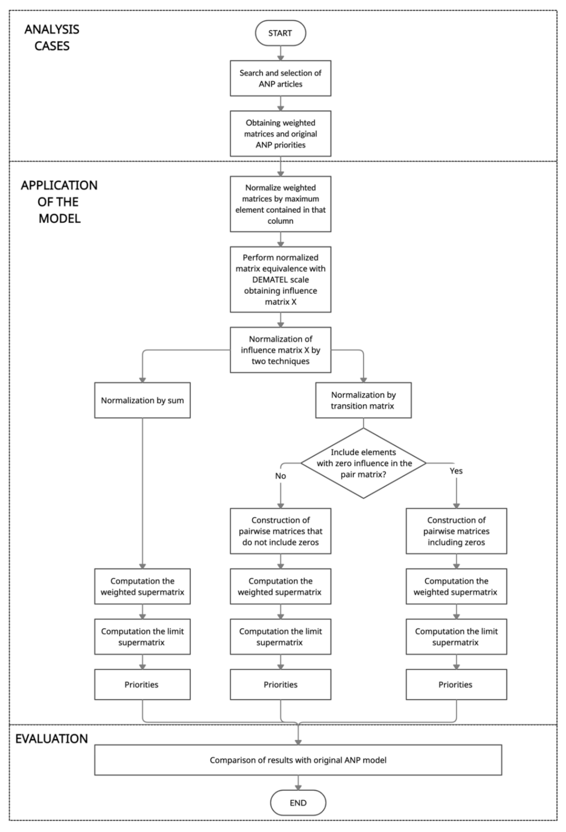
3. Method and Treatments Applied

To contrast the combined DANP proposal of [10] and to check if the results obtained with their proposal are similar to using the ANP, the steps shown in Figure 1 and described below have been followed.

3.1. Searching and Selecting ANP Articles

The first phase carried out was to review the literature to identify articles on ANP applications. To carry this out, the keyword “ANP” or “Analytic Network Process” was used, performing a search in “Abstract, title and keywords” for journal articles in the Scopus database published between 2000 and 2020. In addition, this search has been filtered by subject areas, such as, “Engineering”, “Computer Science”, “Business, Management and Accounting”, “Mathematics”, “Energy”, among others. Conference papers, master’s theses, doctoral dissertations, textbooks and unpublished articles have been discarded from the review process. A total of 603 documents were identified, 237 were discarded for not using the ANP as the applied method. The 366 resulting articles were reviewed to identify whether they included the Weighted Supermatrix, leaving only 87 articles that included it. These 87 articles were reviewed in depth, and those with incomplete models or with matrices with inconsistent data were discarded. A total of 41 articles were finally selected, equivalent to 45 application cases [16,17,18,19,20,21,22,23,24,25,26,27,28,29,30,31,32,33,34,35,36,37,38,39,40,41,42,43,44,45,46,47,48,49,50,51,52,53,54,55,56].

3.2. Calculating Standardised DEMATEL X Matrices

Once the weighted matrices of the ANP applied cases were obtained, they were all converted to influence matrix X (Figure 1) by applying the following process:

• Each column of the Weighted Supermatrix is divided by the maximum value of the column.
• The resulting values are converted to the DEMATEL scale according to

  Table 2. DEMATEL’s equivalent range of influence scale.

  Equivalent Range	DEMATEL Numerical Qualification
  [0, 0.2)	0
  [0.2, 0.4)	1
  [0.4, 0.6)	2
  [0.6, 0.8)	3
  [0.8, 1]	4

  . This matrix is the starting point to apply the analysed proposal.

3.3. Calculating an ANP Weighted Supermatrix from X and Limit Supermatrix

Once the influence matrix X is obtained, the weighted matrix is calculated according to the techniques proposed by Kadoić et al. [10] presented in Section 2.3, as explained below. In all cases, the recommendation to consider all the elements of the ANP model as if they were part of a single cluster has been followed. For each Weighted Supermatrix, its corresponding Limit Supermatrix has been calculated with the influences/priorities of each element of the model.

3.3.1. Normalisation by Sum

As stated above, each column in X is divided by the sum of the column. Therefore, a left stochastic Weighted Supermatrix is directly obtained. As an example, if the matrix X is the one shown in

Table 3. Example of influence matrix X.

	E1	E2	E3	E4	E5
E1	0	2	2	1.33333	2.33333
E2	3.33333	0	2.33333	2	4
E3	0	2.33333	0	3	1.33333
E4	3.33333	0	2.33333	0	1.66667
E5	3	3	1.66667	0	0
Total	9.66666	7.33333	8.33333	6.33333	9.33333

, dividing each value by the sum of its column, the Weighted Supermatrix of

Table 4. Weighted Supermatrix and priorities for the X matrix example, normalisation by sum.

	E1	E2	E3	E4	E5	Priorities
E1	0	0.27273	0.24	0.21053	0.25	0.19464
E2	0.34483	0	0.28	0.31579	0.42857	0.24319
E3	0	0.31818	0	0.47368	0.14286	0.20206
E4	0.34483	0	0.28	0	0.17857	0.14975
E5	0.31035	0.40909	0.2	0	0	0.21037

is obtained. By calculating its Limit Supermatrix, the priorities shown in that same table are obtained.

3.3.2. Transition Matrix

For the calculation by means of a transition matrix, for each column of matrix X a pairwise matrix must be constructed using a transition matrix. The normalised priority vector is located in the corresponding column of the Weighted Supermatrix.

From his article, the following two different procedures for constructing the pairwise comparison matrix are extracted:

1.

To exclude the elements that do not influence the column element from the comparison matrix. This procedure is the one used in the example in the original article.

2.

To include the elements that do not influence the column element in the comparison matrix. This procedure is deduced from the proposed transition matrix since values are included in Saaty’s scale for pairs of values with 0. This procedure should be used if the elements were allowed to influence themselves.

The detailed calculations with the X matrix example of Table 3 using procedure 1 is as follows: Elements E2, E4 and E5 influence element E1. A comparison matrix is built for those three elements. Elements E2 and E4 influence element 1 equally. Subtracting the X values from E2 and E4 in column E1 of Table 3, the result is 0, and according to the proposed transition matrix (Table 1), a 1 must appear in its cells of the comparison matrix (

Table 5. Constructing the pairwise comparison for E1.

E1	E2	E4	E5
E2	1	1
E4	1	1
E5			1

).

When studying the influence on E1 of another couple of elements the following can be observed: E2 influences 0.34483 on E1, while E5 influences 0.31035. The difference is 0.3333 if E2 is compared with E5, and 0.3333 if E5 is compared with E2. Interpolating the value 0.3333 according to the transition matrix, the value 1.6666 is obtained for the cell (E2, E5). Its reciprocal value for cell (E5, E2) is 0.6. A different result is obtained if the value 0.3333 is interpolated and then its reciprocal is calculated: 0.7778 for cell (E5, E2) and its reciprocal 1.2857 for cell (E2, E5).

Kadoić et al. [10] do not indicate exactly the calculations to be carried out to construct the pairwise matrix. This article provides the following three different options for constructing pairwise matrices:

(a)

Obtaining the judgments in the entries above the main diagonal with the transition matrix and filling the lower left half of the matrix with the corresponding fractions. In this way, the pairwise comparison matrix for element E1 of Table 3 would be as shown in

Table 6. Pairwise comparison matrix of element E1, for the matrix X example, according to procedure 1 variant (a).

E1	E2	E4	E5	Influence
E2	1	1	1.66666	0.38462
E4	1	1	1.66666	0.38462
E5	0.6000024	0.6000024	1	0.23077

, where the resulting influences are also indicated.

These influence values are located in their corresponding cells in the Weighted Supermatrix. Repeating the process for the rest of the columns of matrix X, the Weighted Supermatrix is obtained (

Table 7. Weighted Supermatrix and priorities according to procedure 1 variant (a).

	E1	E2	E3	E4	E5	Priorities
E1	0	0.19405	0.23803	0.14028	0.20293	0.16455
E2	0.38462	0	0.31255	0.23019	0.61977	0.28918
E3	0	0.27204	0	0.62953	0.07935	0.18578
E4	0.38462	0	0.31255	0	0.09795	0.14269
E5	0.23077	0.53391	0.13687	0	0	0.2178

).

(b)

Obtaining the judgments in the entries below the main diagonal with the transition matrix and filling the upper right half of the matrix with the corresponding fractions. In this way, the pairwise comparison matrix for element E1 of Table 3 would be as shown in

Table 8. Pairwise comparison matrix of element E1, for the example of matrix X, according to procedure 1 variant (b).

E1	E2	E4	E5	Influence
E2	1	1	1.285711	0.36
E4	1	1	1.285711	0.36
E5	0.77778	0.77778	1	0.28

, where the resulting influences are also indicated. Repeating the already known process, the Weighted Supermatrix is obtained (

Table 9. Weighted Supermatrix and priorities according to procedure 1 variant (b).

	E1	E2	E3	E4	E5	Priorities
E1	0	0.17243	0.19855	0.12387	0.18795	0.14856
E2	0.36	0	0.31649	0.24633	0.62379	0.29348
E3	0	0.26356	0	0.62981	0.07573	0.18222
E4	0.36	0	0.31649	0	0.11254	0.13792
E5	0.28	0.56401	0.16848	0	0	0.23782

).

(c)

Obtaining both previous matrices and calculating their geometric mean. This is equivalent to considering each pairwise matrix as if it were issued by a decision maker. In this way, the pairwise comparison matrix for element E1 of Table 3 would be as shown in

Table 10. Pairwise comparison matrix of element E1, for matrix X example, according to procedure 1 variant (c).

E1	E2	E4	E5	Influence
E2	1	1	1.463845	0.3727
E4	1	1	1.463845	0.3727
E5	0.6831324	0.6831324	1	0.2546

, where the resulting influences are also indicated. Repeating the already known process, the Weighted Supermatrix is obtained (

Table 11. Weighted Supermatrix and priorities according to procedure 1 per variant (c).

	E1	E2	E3	E4	E5	Priorities
E1	0	0.18302	0.21769	0.13187	0.19544	0.15643
E2	0.3727	0	0.31512	0.23821	0.622	0.29142
E3	0	0.26791	0	0.62991	0.07755	0.18408
E4	0.3727	0	0.31512	0	0.10502	0.14023
E5	0.2546	0.54906	0.15207	0	0	0.22783

).

These three ways of calculating pairwise matrices result in different pairwise matrices, and, therefore, a different Weighted Supermatrix, when the values in the X matrix do not correspond to an integer value on the DEMATEL scale. For example, when that matrix X is matrix A of the DEMATEL method, obtained as an average of the X matrices of various experts; or when a single expert uses intermediate values of the DEMATEL scale.

In this article, in the cases where the transition matrix is applied, due to the way of calculating the X matrix explained in step 3.2, the three ways of calculating the pairwise matrices give the same result, since there was only a single X matrix and with integer values on the DEMATEL scale. However, it is important to point out that method (c) seems more in line with the philosophy that Saaty inspires in his AHP/ANP proposal.

These three variants are also present when including the elements that have 0 influence in the pairwise comparison matrices. Continuing with the example of matrix X from Table 3,

Table 12. Pairwise comparison matrix of element E1, for matrix X example, according to procedure 2 variant (a).

E1	E1	E2	E3	E4	E5	Influence
E1	1	0.1322752	1	0.1322752	0.1428571	0.0409
E2	7.559994	1	7.66666	1	1.66666	0.33835
E3	1	0.1304349	1	0.1322752	0.1428571	0.04078
E4	7.559994	1	7.559994	1	1.66666	0.33748
E5	7	0.6000024	7	0.6000024	1	0.2425

,

Table 13. Weighted Supermatrix and priorities according to procedure 2 variant (a).

	E1	E2	E3	E4	E5	Priorities
E1	0.0409	0.2061	0.22846	0.15509	0.20575	0.17352
E2	0.33835	0.04909	0.29218	0.23595	0.56078	0.27882
E3	0.04078	0.25982	0.04585	0.50481	0.08903	0.18542
E4	0.33748	0.04886	0.2909	0.05208	0.10899	0.15668
E5	0.2425	0.43613	0.1426	0.05208	0.03545	0.20557

,

Table 14. Pairwise comparison matrix of element E1, for matrix X example, according to procedure 2 variant (b).

E1	E1	E2	E3	E4	E5	Influence
E1	1	0.1304349	1	0.1304349	0.1428571	0.041
E2	7.66666	1	7.559994	1	1.2857106	0.32375
E3	1	0.1322752	1	0.1304349	0.1428571	0.04112
E4	7.66666	1	7.66666	1	1.2857106	0.32462
E5	7	0.77778	7	0.77778	1	0.2695

,

Table 15. Weighted Supermatrix and priorities according to variant (b).

	E1	E2	E3	E4	E5	Priorities
E1	0.041	0.19257	0.19813	0.14169	0.19296	0.16136
E2	0.32375	0.04815	0.29323	0.24767	0.56536	0.28148
E3	0.04112	0.25779	0.04561	0.50634	0.08506	0.18444
E4	0.32462	0.04838	0.2945	0.05215	0.12018	0.15459
E5	0.2695	0.45311	0.16853	0.05215	0.03644	0.21812

,

Table 16. Pairwise comparison matrix of element E1, for matrix X example, according to variant (c).

E1	E1	E2	E3	E4	E5	Influence
E1	1	0.1313518	1	0.1313518	0.1428571	0.04098
E2	7.61314	1	7.61314	1	1.4638451	0.33119
E3	1	0.1313518	1	0.1313518	0.1428571	0.04098
E4	7.61314	1	7.61314	1	1.4638451	0.33119
E5	7	0.6831324	7	0.6831324	1	0.25566

and

Table 17. Weighted Supermatrix and priorities according to variant (c).

	E1	E2	E3	E4	E5	Priorities
E1	0.04098	0.19936	0.21291	0.14826	0.19931	0.16739
E2	0.33119	0.0487	0.29307	0.24172	0.5633	0.28021
E3	0.04098	0.25875	0.04578	0.50575	0.08705	0.18498
E4	0.33119	0.0487	0.29307	0.05214	0.1144	0.15564
E5	0.25566	0.44449	0.15517	0.05214	0.03595	0.21178

show the pairwise comparison matrices for column E1, the Weighted Supermatrices and the priorities, according to variants (a–c).

3.4. Comparison of the Results of ANP–DEMATEL Integration Normalisation Techniques with Respect to ANP

Finally, the two priority results obtained using the proposed combination of ANP–DEMATEL have been compared with the published prioritisation obtained by the conventional ANP method.

The following different indicators have been proposed to measure how similar two vectors are, some based on rank, and others on priority values: Saaty’s Compatibility Index based on the Hadamard product [3]; the Garuti’s Compatibility index [57,58]; Salabun and Urbaniak proposed the WS coefficient [59] and compared it with Spearman, Kendall, Goodman-Kruskal and Blest coefficients.

In this paper, Spearman’s rank correlation coefficient and the mean squared error (MSE) are calculated for each of the cases analysed, because those are the indicators that the authors use in their proposal to compare both results, normalised by the sum and transition matrix.

The number of questions to be answered has also been calculated using the original ANP and the new method proposed in [10].

4. Case Study and Application

This section presents case one of the 45 case studies to which the evaluated proposal has been applied. The remaining cases with their respective tables are included in the Supplementary Materials of the article. Case one corresponds to the article [16].

4.1. Standardization to Determine Influences between Criteria

Table 18. Case 1. Original Weighted Supermatrix.

	CL1	CL2				CL3					CL4	CL5			CL6					CL7	CL8
	E1	E2	E3	E4	E5	E6	E7	E8	E9	E10	E11	E12	E13	E14	E15	E16	E17	E18	E19	E20	E21
E1	0.000	0.000	0.109	0.000	0.000	0.000	0.000	0.000	0.000	0.000	0.062	0.054	0.087	0.000	0.177	0.181	0.179	0.202	0.179	0.064	0.165
E2	0.000	0.000	0.293	1.000	0.097	0.024	0.028	0.030	0.000	0.000	0.000	0.035	0.068	0.024	0.019	0.035	0.023	0.015	0.020	0.016	0.029
E3	0.000	0.025	0.000	0.000	0.042	0.000	0.000	0.000	0.000	0.000	0.000	0.000	0.000	0.000	0.014	0.000	0.000	0.015	0.025	0.016	0.029
E4	0.000	0.120	0.123	0.000	0.037	0.024	0.022	0.030	0.030	0.052	0.079	0.035	0.023	0.030	0.011	0.009	0.009	0.015	0.008	0.016	0.029
E5	0.000	0.032	0.077	0.000	0.000	0.000	0.000	0.000	0.030	0.000	0.079	0.000	0.023	0.077	0.008	0.009	0.020	0.015	0.000	0.016	0.029
E6	0.011	0.022	0.000	0.000	0.046	0.000	0.050	0.094	0.152	0.070	0.069	0.021	0.032	0.063	0.048	0.024	0.047	0.036	0.015	0.019	0.006
E7	0.008	0.018	0.000	0.000	0.021	0.027	0.000	0.048	0.192	0.122	0.077	0.058	0.058	0.251	0.085	0.114	0.147	0.223	0.110	0.114	0.019
E8	0.023	0.079	0.000	0.000	0.114	0.160	0.149	0.000	0.241	0.319	0.107	0.059	0.105	0.251	0.140	0.136	0.131	0.199	0.154	0.112	0.068
E9	0.098	0.200	0.000	0.000	0.221	0.137	0.149	0.211	0.000	0.000	0.196	0.163	0.202	0.000	0.128	0.026	0.000	0.000	0.059	0.104	0.045
E10	0.019	0.084	0.000	0.000	0.000	0.147	0.149	0.232	0.000	0.000	0.116	0.000	0.088	0.000	0.000	0.110	0.082	0.000	0.068	0.000	0.040
E11	0.160	0.237	0.000	0.000	0.237	0.286	0.302	0.356	0.356	0.311	0.000	0.123	0.197	0.229	0.204	0.209	0.207	0.233	0.207	0.364	0.218
E12	0.004	0.005	0.000	0.000	0.000	0.015	0.012	0.000	0.000	0.000	0.000	0.000	0.011	0.057	0.000	0.000	0.000	0.000	0.056	0.025	0.018
E13	0.010	0.019	0.000	0.000	0.021	0.007	0.000	0.000	0.000	0.062	0.000	0.010	0.000	0.019	0.110	0.112	0.111	0.000	0.056	0.025	0.016
E14	0.012	0.017	0.000	0.000	0.021	0.035	0.048	0.000	0.000	0.000	0.108	0.030	0.054	0.000	0.000	0.000	0.000	0.000	0.000	0.025	0.081
E15	0.013	0.016	0.219	0.000	0.000	0.012	0.000	0.000	0.000	0.000	0.000	0.064	0.000	0.000	0.000	0.000	0.000	0.000	0.011	0.030	0.016
E16	0.002	0.005	0.000	0.000	0.000	0.002	0.031	0.000	0.000	0.032	0.053	0.012	0.000	0.000	0.000	0.000	0.043	0.049	0.011	0.024	0.002
E17	0.003	0.006	0.000	0.000	0.104	0.002	0.031	0.000	0.000	0.032	0.053	0.013	0.000	0.000	0.000	0.000	0.000	0.000	0.011	0.022	0.003
E18	0.007	0.007	0.073	0.000	0.000	0.003	0.000	0.000	0.000	0.000	0.000	0.000	0.000	0.000	0.007	0.000	0.000	0.000	0.011	0.007	0.004
E19	0.043	0.070	0.000	0.000	0.000	0.041	0.000	0.000	0.000	0.000	0.000	0.050	0.000	0.000	0.035	0.000	0.000	0.000	0.000	0.000	0.080
E20	0.043	0.038	0.107	0.000	0.038	0.026	0.028	0.000	0.000	0.000	0.000	0.033	0.053	0.000	0.013	0.000	0.000	0.000	0.000	0.000	0.102
E21	0.543	0.000	0.000	0.000	0.000	0.053	0.000	0.000	0.000	0.000	0.000	0.239	0.000	0.000	0.000	0.035	0.000	0.000	0.000	0.000	0.000

shows the original Weighted Supermatrix of case one obtained from the bibliographic review process presented in the previous section. This case presents a public works bidding process with an ANP network structure with 21 elements in 8 clusters. Using the ANP, this model needs 441 questions to identify the relationships between elements, 268 questions to prioritize the relationships between the nodes and obtain the Unweighted Supermatrix, and 159 questions to obtain the cluster matrix, and be able to calculate the Weighted Supermatrix. Using the Kadoić et al. proposal and their recommendation to consider all the elements in a single cluster, 441 questions are needed to identify the relationships and prioritize the influences between the elements and obtain the Weighted Supermatrix. If there were interest in considering the 8 clusters and obtain their cluster matrix, with the proposal of Kadoić et al. only 54 additional questions would be needed.

Each column of the weighted matrix is divided by the maximum element contained in that same column (

Table 19. Case 1. Original Weighted Supermatrix divided by the maximum of each column.

	CL1	CL2				CL3					CL4	CL5			CL6					CL7	CL8
	E1	E2	E3	E4	E5	E6	E7	E8	E9	E10	E11	E12	E13	E14	E15	E16	E17	E18	E19	E20	E21
E1	0.000	0.000	0.371	0.000	0.000	0.000	0.000	0.000	0.000	0.000	0.317	0.227	0.441	0.000	0.867	0.867	0.867	0.867	0.867	0.177	0.757
E2	0.000	0.000	1.000	1.000	0.409	0.083	0.092	0.083	0.000	0.000	0.000	0.147	0.344	0.096	0.095	0.170	0.113	0.064	0.096	0.043	0.134
E3	0.000	0.106	0.000	0.000	0.179	0.000	0.000	0.000	0.000	0.000	0.000	0.000	0.000	0.000	0.069	0.000	0.000	0.064	0.121	0.043	0.134
E4	0.000	0.504	0.420	0.000	0.156	0.083	0.074	0.083	0.083	0.162	0.401	0.147	0.115	0.122	0.052	0.042	0.043	0.064	0.038	0.043	0.134
E5	0.000	0.133	0.265	0.000	0.000	0.000	0.000	0.000	0.083	0.000	0.401	0.000	0.115	0.306	0.038	0.042	0.099	0.064	0.000	0.043	0.134
E6	0.020	0.091	0.000	0.000	0.192	0.000	0.164	0.263	0.427	0.218	0.351	0.090	0.162	0.250	0.236	0.114	0.229	0.153	0.074	0.054	0.029
E7	0.015	0.076	0.000	0.000	0.089	0.094	0.000	0.135	0.538	0.382	0.393	0.244	0.293	1.000	0.415	0.547	0.708	0.956	0.533	0.314	0.085
E8	0.042	0.332	0.000	0.000	0.482	0.559	0.493	0.000	0.678	1.000	0.543	0.248	0.534	1.000	0.688	0.651	0.633	0.855	0.744	0.307	0.311
E9	0.180	0.844	0.000	0.000	0.933	0.477	0.493	0.592	0.000	0.000	1.000	0.681	1.024	0.000	0.626	0.124	0.000	0.000	0.285	0.287	0.207
E10	0.034	0.353	0.000	0.000	0.000	0.512	0.493	0.653	0.000	0.000	0.593	0.000	0.448	0.000	0.000	0.528	0.394	0.000	0.328	0.000	0.184
E11	0.295	1.000	0.000	0.000	1.000	1.000	1.000	1.000	1.000	0.974	0.000	0.513	1.000	0.914	1.000	1.000	1.000	1.000	1.000	1.000	1.000
E12	0.008	0.022	0.000	0.000	0.000	0.054	0.040	0.000	0.000	0.000	0.000	0.000	0.055	0.226	0.000	0.000	0.000	0.000	0.268	0.070	0.081
E13	0.019	0.081	0.000	0.000	0.088	0.023	0.000	0.000	0.000	0.195	0.000	0.042	0.000	0.075	0.537	0.537	0.537	0.000	0.268	0.070	0.071
E14	0.022	0.074	0.000	0.000	0.088	0.123	0.160	0.000	0.000	0.000	0.552	0.127	0.275	0.000	0.000	0.000	0.000	0.000	0.000	0.070	0.372
E15	0.024	0.068	0.748	0.000	0.000	0.041	0.000	0.000	0.000	0.000	0.000	0.270	0.000	0.000	0.000	0.000	0.000	0.000	0.052	0.083	0.072
E16	0.004	0.023	0.000	0.000	0.000	0.006	0.104	0.000	0.000	0.102	0.272	0.048	0.000	0.000	0.000	0.000	0.209	0.209	0.052	0.066	0.010
E17	0.006	0.024	0.000	0.000	0.440	0.007	0.104	0.000	0.000	0.102	0.272	0.054	0.000	0.000	0.000	0.000	0.000	0.000	0.052	0.060	0.013
E18	0.014	0.029	0.249	0.000	0.000	0.011	0.000	0.000	0.000	0.000	0.000	0.000	0.000	0.000	0.035	0.000	0.000	0.000	0.052	0.019	0.020
E19	0.080	0.296	0.000	0.000	0.000	0.144	0.000	0.000	0.000	0.000	0.000	0.211	0.000	0.000	0.174	0.000	0.000	0.000	0.000	0.000	0.364
E20	0.079	0.161	0.365	0.000	0.161	0.092	0.092	0.000	0.000	0.000	0.000	0.138	0.268	0.000	0.066	0.000	0.000	0.000	0.000	0.000	0.465
E21	1.000	0.000	0.000	0.000	0.000	0.187	0.000	0.000	0.000	0.000	0.000	1.000	0.000	0.000	0.000	0.167	0.000	0.000	0.000	0.000	0.000
Sum	1.841	4.218	3.417	1.000	4.218	3.495	3.308	2.808	2.808	3.133	5.096	4.187	5.073	3.990	4.897	4.790	4.832	4.295	4.832	2.750	4.578

) to later convert it through the equivalence of values with the DEMATEL scale (0–4), resulting in the influence matrix X for case one (see

Table 20. Case 1’s X Influence Matrix.

	CL1	CL2				CL3					CL4	CL5			CL6					CL7	CL8
	E1	E2	E3	E4	E5	E6	E7	E8	E9	E10	E11	E12	E13	E14	E15	E16	E17	E18	E19	E20	E21
E1	0	0	1	0	0	0	0	0	0	0	1	1	2	0	4	4	4	4	4	0	3
E2	0	0	4	4	2	0	0	0	0	0	0	0	1	0	0	0	0	0	0	0	0
E3	0	0	0	0	0	0	0	0	0	0	0	0	0	0	0	0	0	0	0	0	0
E4	0	2	2	0	0	0	0	0	0	0	2	0	0	0	0	0	0	0	0	0	0
E5	0	0	1	0	0	0	0	0	0	0	2	0	0	1	0	0	0	0	0	0	0
E6	0	0	0	0	0	0	0	1	2	1	1	0	0	1	1	0	1	0	0	0	0
E7	0	0	0	0	0	0	0	0	2	1	1	1	1	4	2	2	3	4	2	1	0
E8	0	1	0	0	2	2	2	0	3	4	2	1	2	4	3	3	3	4	3	1	1
E9	0	4	0	0	4	2	2	2	0	0	4	3	4	0	3	0	0	0	1	1	1
E10	0	1	0	0	0	2	2	3	0	0	2	0	2	0	0	2	1	0	1	0	0
E11	1	4	0	0	4	4	4	4	4	4	0	2	4	4	4	4	4	4	4	4	4
E12	0	0	0	0	0	0	0	0	0	0	0	0	0	1	0	0	0	0	1	0	0
E13	0	0	0	0	0	0	0	0	0	0	0	0	0	0	2	2	2	0	1	0	0
E14	0	0	0	0	0	0	0	0	0	0	2	0	1	0	0	0	0	0	0	0	1
E15	0	0	3	0	0	0	0	0	0	0	0	1	0	0	0	0	0	0	0	0	0
E16	0	0	0	0	0	0	0	0	0	0	1	0	0	0	0	0	1	1	0	0	0
E17	0	0	0	0	2	0	0	0	0	0	1	0	0	0	0	0	0	0	0	0	0
E18	0	0	1	0	0	0	0	0	0	0	0	0	0	0	0	0	0	0	0	0	0
E19	0	1	0	0	0	0	0	0	0	0	0	1	0	0	0	0	0	0	0	0	1
E20	0	0	1	0	0	0	0	0	0	0	0	0	1	0	0	0	0	0	0	0	2
E21	4	0	0	0	0	0	0	0	0	0	0	4	0	0	0	0	0	0	0	0	0

).

4.2. Normalisation by Sum and Obtaining the Limit Supermatrix

Once the influence matrix X is obtained for case one, each element is normalised by the sum of its respective column, obtaining a stochastic Weighted Supermatrix (

Table 21. Case 1. Weighted Supermatrix normalisation by sum and priorities.

	CL1	CL2				CL3					CL4		CL5		CL6					CL7	CL8
	E1	E2	E3	E4	E5	E6	E7	E8	E9	E10	E11	E12	E13	E14	E15	E16	E17	E18	E19	E20	E21	Priorities
E1	0.000	0.000	0.077	0.000	0.000	0.000	0.000	0.000	0.000	0.000	0.053	0.071	0.111	0.000	0.211	0.235	0.211	0.235	0.235	0.000	0.231	0.027
E2	0.000	0.000	0.308	1.000	0.143	0.000	0.000	0.000	0.000	0.000	0.000	0.000	0.056	0.000	0.000	0.000	0.000	0.000	0.000	0.000	0.000	0.037
E3	0.000	0.000	0.000	0.000	0.000	0.000	0.000	0.000	0.000	0.000	0.000	0.000	0.000	0.000	0.000	0.000	0.000	0.000	0.000	0.000	0.000	0.000
E4	0.000	0.154	0.154	0.000	0.000	0.000	0.000	0.000	0.000	0.000	0.105	0.000	0.000	0.000	0.000	0.000	0.000	0.000	0.000	0.000	0.000	0.033
E5	0.000	0.000	0.077	0.000	0.000	0.000	0.000	0.000	0.000	0.000	0.105	0.000	0.000	0.067	0.000	0.000	0.000	0.000	0.000	0.000	0.000	0.029
E6	0.000	0.000	0.000	0.000	0.000	0.000	0.000	0.100	0.182	0.100	0.053	0.000	0.000	0.067	0.053	0.000	0.053	0.000	0.000	0.000	0.000	0.067
E7	0.000	0.000	0.000	0.000	0.000	0.000	0.000	0.000	0.182	0.100	0.053	0.071	0.056	0.267	0.105	0.118	0.158	0.235	0.118	0.143	0.000	0.062
E8	0.000	0.077	0.000	0.000	0.143	0.200	0.200	0.000	0.273	0.400	0.105	0.071	0.111	0.267	0.158	0.176	0.158	0.235	0.176	0.143	0.077	0.155
E9	0.000	0.308	0.000	0.000	0.286	0.200	0.200	0.200	0.000	0.000	0.211	0.214	0.222	0.000	0.158	0.000	0.000	0.000	0.059	0.143	0.077	0.134
E10	0.000	0.077	0.000	0.000	0.000	0.200	0.200	0.300	0.000	0.000	0.105	0.000	0.111	0.000	0.000	0.118	0.053	0.000	0.059	0.000	0.000	0.105
E11	0.200	0.308	0.000	0.000	0.286	0.400	0.400	0.400	0.364	0.400	0.000	0.143	0.222	0.267	0.211	0.235	0.211	0.235	0.235	0.571	0.308	0.255
E12	0.000	0.000	0.000	0.000	0.000	0.000	0.000	0.000	0.000	0.000	0.000	0.000	0.000	0.067	0.000	0.000	0.000	0.000	0.059	0.000	0.000	0.002
E13	0.000	0.000	0.000	0.000	0.000	0.000	0.000	0.000	0.000	0.000	0.000	0.000	0.000	0.000	0.105	0.118	0.105	0.000	0.059	0.000	0.000	0.004
E14	0.000	0.000	0.000	0.000	0.000	0.000	0.000	0.000	0.000	0.000	0.105	0.000	0.056	0.000	0.000	0.000	0.000	0.000	0.000	0.000	0.077	0.029
E15	0.000	0.000	0.231	0.000	0.000	0.000	0.000	0.000	0.000	0.000	0.000	0.071	0.000	0.000	0.000	0.000	0.000	0.000	0.000	0.000	0.000	0.000
E16	0.000	0.000	0.000	0.000	0.000	0.000	0.000	0.000	0.000	0.000	0.053	0.000	0.000	0.000	0.000	0.000	0.053	0.059	0.000	0.000	0.000	0.014
E17	0.000	0.000	0.000	0.000	0.143	0.000	0.000	0.000	0.000	0.000	0.053	0.000	0.000	0.000	0.000	0.000	0.000	0.000	0.000	0.000	0.000	0.018
E18	0.000	0.000	0.077	0.000	0.000	0.000	0.000	0.000	0.000	0.000	0.000	0.000	0.000	0.000	0.000	0.000	0.000	0.000	0.000	0.000	0.000	0.000
E19	0.000	0.077	0.000	0.000	0.000	0.000	0.000	0.000	0.000	0.000	0.000	0.071	0.000	0.000	0.000	0.000	0.000	0.000	0.000	0.000	0.077	0.005
E20	0.000	0.000	0.077	0.000	0.000	0.000	0.000	0.000	0.000	0.000	0.000	0.000	0.056	0.000	0.000	0.000	0.000	0.000	0.000	0.000	0.154	0.004
E21	0.800	0.000	0.000	0.000	0.000	0.000	0.000	0.000	0.000	0.000	0.000	0.286	0.000	0.000	0.000	0.000	0.000	0.000	0.000	0.000	0.000	0.023

). Subsequently, the Limit Supermatrix is calculated, and the priorities of the elements are obtained (Table 21).

4.3. Normalisation by Matrix of Transition and Obtaining Limit Matrix

Using as a basis the influence matrix X obtained in Section 4.1 (Table 20), the transition matrix (Table 1) is used to obtain the values of the Weighted Supermatrix. Each column in the Weighted Supermatrix is calculated using a paired matrix with the elements in the row that influence each column. As shown above, two different procedures can be used to build the comparison matrix, with three variants in each case. As already mentioned in this study, the three construction variants of the pairwise comparison matrices result in the same comparison matrix because the X matrices have integer values of the DEMATEL scale. Thus, for each of the 45 cases, two Weighted Supermatrices have been calculated, following procedures one and two.

Next, the procedure to calculate the first column of the Weighted Supermatrix of case one, using the transition matrix for both procedures, will be shown as an example.

Table 22. Case 1. E1 Pairwise Comparison Matrix and Eigenvector according to procedure 1.

E1	E11	E21	Normalised Eigenvector
E11	1.000	0.143	0.125
E21	7.000	1.000	0.875

shows the pairwise comparison matrix for column one corresponding to element E1, following procedure one. Once the comparison matrix has been obtained as a function of the intensity of its influences, the normalised principal eigenvector is calculated (Table 22). This eigenvector corresponds to the first column of the Weighted Supermatrix, as can be seen in

Table 23. Case 1. Weighted Supermatrix and priorities, according to procedure 1.

	E1	E2	E3	E4	E5	E6	E7	E8	E9	E10	E11	E12	E13	E14	E15	E16	E17	E18	E19	E20	E21	Priorities
E1	0.000	0.000	0.049	0.000	0.000	0.000	0.000	0.000	0.000	0.000	0.034	0.047	0.085	0.000	0.299	0.334	0.286	0.241	0.306	0.000	0.242	0.025
E2	0.000	0.000	0.440	1.000	0.077	0.000	0.000	0.000	0.000	0.000	0.000	0.000	0.033	0.000	0.000	0.000	0.000	0.000	0.000	0.000	0.000	0.037
E3	0.000	0.000	0.000	0.000	0.000	0.000	0.000	0.000	0.000	0.000	0.000	0.000	0.000	0.000	0.000	0.000	0.000	0.000	0.000	0.000	0.000	0.000
E4	0.000	0.112	0.123	0.000	0.000	0.000	0.000	0.000	0.000	0.000	0.095	0.000	0.000	0.000	0.000	0.000	0.000	0.000	0.000	0.000	0.000	0.034
E5	0.000	0.000	0.049	0.000	0.000	0.000	0.000	0.000	0.000	0.000	0.095	0.000	0.000	0.042	0.000	0.000	0.000	0.000	0.000	0.000	0.000	0.032
E6	0.000	0.000	0.000	0.000	0.000	0.000	0.000	0.055	0.095	0.063	0.034	0.000	0.000	0.042	0.028	0.000	0.030	0.000	0.000	0.000	0.000	0.041
E7	0.000	0.000	0.000	0.000	0.000	0.000	0.000	0.000	0.095	0.063	0.034	0.047	0.033	0.292	0.056	0.060	0.136	0.241	0.084	0.100	0.000	0.044
E8	0.000	0.047	0.000	0.000	0.077	0.125	0.125	0.000	0.249	0.438	0.095	0.047	0.085	0.292	0.131	0.151	0.136	0.241	0.162	0.100	0.049	0.136
E9	0.000	0.374	0.000	0.000	0.385	0.125	0.125	0.118	0.000	0.000	0.353	0.234	0.307	0.000	0.131	0.000	0.000	0.000	0.035	0.100	0.049	0.167
E10	0.000	0.047	0.000	0.000	0.000	0.125	0.125	0.262	0.000	0.000	0.095	0.000	0.085	0.000	0.000	0.060	0.030	0.000	0.035	0.000	0.000	0.080
E11	0.125	0.374	0.000	0.000	0.385	0.625	0.625	0.565	0.560	0.438	0.000	0.121	0.307	0.292	0.299	0.334	0.286	0.241	0.306	0.700	0.440	0.317
E12	0.000	0.000	0.000	0.000	0.000	0.000	0.000	0.000	0.000	0.000	0.000	0.000	0.000	0.042	0.000	0.000	0.000	0.000	0.035	0.000	0.000	0.001
E13	0.000	0.000	0.000	0.000	0.000	0.000	0.000	0.000	0.000	0.000	0.000	0.000	0.000	0.000	0.056	0.060	0.066	0.000	0.035	0.000	0.000	0.002
E14	0.000	0.000	0.000	0.000	0.000	0.000	0.000	0.000	0.000	0.000	0.095	0.000	0.033	0.000	0.000	0.000	0.000	0.000	0.000	0.000	0.049	0.031
E15	0.000	0.000	0.242	0.000	0.000	0.000	0.000	0.000	0.000	0.000	0.000	0.047	0.000	0.000	0.000	0.000	0.000	0.000	0.000	0.000	0.000	0.000
E16	0.000	0.000	0.000	0.000	0.000	0.000	0.000	0.000	0.000	0.000	0.034	0.000	0.000	0.000	0.000	0.000	0.030	0.034	0.000	0.000	0.000	0.011
E17	0.000	0.000	0.000	0.000	0.077	0.000	0.000	0.000	0.000	0.000	0.034	0.000	0.000	0.000	0.000	0.000	0.000	0.000	0.000	0.000	0.000	0.013
E18	0.000	0.000	0.049	0.000	0.000	0.000	0.000	0.000	0.000	0.000	0.000	0.000	0.000	0.000	0.000	0.000	0.000	0.000	0.000	0.000	0.000	0.000
E19	0.000	0.047	0.000	0.000	0.000	0.000	0.000	0.000	0.000	0.000	0.000	0.047	0.000	0.000	0.000	0.000	0.000	0.000	0.000	0.000	0.049	0.003
E20	0.000	0.000	0.049	0.000	0.000	0.000	0.000	0.000	0.000	0.000	0.000	0.000	0.033	0.000	0.000	0.000	0.000	0.000	0.000	0.000	0.123	0.003
E21	0.875	0.000	0.000	0.000	0.000	0.000	0.000	0.000	0.000	0.000	0.000	0.412	0.000	0.000	0.000	0.000	0.000	0.000	0.000	0.000	0.000	0.022

.

The Limit Supermatrix is calculated in the same way as with the normalisation by the sum, obtaining the priorities of the elements (see Table 23).

Following procedure two, the comparison matrix for element E1 and priorities from

Table 24. Case 1. E1 Pairwise Comparison Matrix and Eigenvector according to procedure 2.

E1	E1	E2	E3	E4	E5	E6	E7	E8	E9	E10	E11	E12	E13	E14	E15	E16	E17	E18	E19	E20	E21	Priorities
E1	1.000	1.000	1.000	1.000	1.000	1.000	1.000	1.000	1.000	1.000	0.333	1.000	1.000	1.000	1.000	1.000	1.000	1.000	1.000	1.000	0.111	0.032
E2	1.000	1.000	1.000	1.000	1.000	1.000	1.000	1.000	1.000	1.000	0.333	1.000	1.000	1.000	1.000	1.000	1.000	1.000	1.000	1.000	0.111	0.032
E3	1.000	1.000	1.000	1.000	1.000	1.000	1.000	1.000	1.000	1.000	0.333	1.000	1.000	1.000	1.000	1.000	1.000	1.000	1.000	1.000	0.111	0.032
E4	1.000	1.000	1.000	1.000	1.000	1.000	1.000	1.000	1.000	1.000	0.333	1.000	1.000	1.000	1.000	1.000	1.000	1.000	1.000	1.000	0.111	0.032
E5	1.000	1.000	1.000	1.000	1.000	1.000	1.000	1.000	1.000	1.000	0.333	1.000	1.000	1.000	1.000	1.000	1.000	1.000	1.000	1.000	0.111	0.032
E6	1.000	1.000	1.000	1.000	1.000	1.000	1.000	1.000	1.000	1.000	0.333	1.000	1.000	1.000	1.000	1.000	1.000	1.000	1.000	1.000	0.111	0.032
E7	1.000	1.000	1.000	1.000	1.000	1.000	1.000	1.000	1.000	1.000	0.333	1.000	1.000	1.000	1.000	1.000	1.000	1.000	1.000	1.000	0.111	0.032
E8	1.000	1.000	1.000	1.000	1.000	1.000	1.000	1.000	1.000	1.000	0.333	1.000	1.000	1.000	1.000	1.000	1.000	1.000	1.000	1.000	0.111	0.032
E9	1.000	1.000	1.000	1.000	1.000	1.000	1.000	1.000	1.000	1.000	0.333	1.000	1.000	1.000	1.000	1.000	1.000	1.000	1.000	1.000	0.111	0.032
E10	1.000	1.000	1.000	1.000	1.000	1.000	1.000	1.000	1.000	1.000	0.333	1.000	1.000	1.000	1.000	1.000	1.000	1.000	1.000	1.000	0.111	0.032
E11	3.000	3.000	3.000	3.000	3.000	3.000	3.000	3.000	3.000	3.000	1.000	3.000	3.000	3.000	3.000	3.000	3.000	3.000	3.000	3.000	0.143	0.032
E12	1.000	1.000	1.000	1.000	1.000	1.000	1.000	1.000	1.000	1.000	0.333	1.000	1.000	1.000	1.000	1.000	1.000	1.000	1.000	1.000	0.111	0.032
E13	1.000	1.000	1.000	1.000	1.000	1.000	1.000	1.000	1.000	1.000	0.333	1.000	1.000	1.000	1.000	1.000	1.000	1.000	1.000	1.000	0.111	0.032
E14	1.000	1.000	1.000	1.000	1.000	1.000	1.000	1.000	1.000	1.000	0.333	1.000	1.000	1.000	1.000	1.000	1.000	1.000	1.000	1.000	0.111	0.032
E15	1.000	1.000	1.000	1.000	1.000	1.000	1.000	1.000	1.000	1.000	0.333	1.000	1.000	1.000	1.000	1.000	1.000	1.000	1.000	1.000	0.111	0.032
E16	1.000	1.000	1.000	1.000	1.000	1.000	1.000	1.000	1.000	1.000	0.333	1.000	1.000	1.000	1.000	1.000	1.000	1.000	1.000	1.000	0.111	0.032
E17	1.000	1.000	1.000	1.000	1.000	1.000	1.000	1.000	1.000	1.000	0.333	1.000	1.000	1.000	1.000	1.000	1.000	1.000	1.000	1.000	0.111	0.032
E18	1.000	1.000	1.000	1.000	1.000	1.000	1.000	1.000	1.000	1.000	0.333	1.000	1.000	1.000	1.000	1.000	1.000	1.000	1.000	1.000	0.111	0.032
E19	1.000	1.000	1.000	1.000	1.000	1.000	1.000	1.000	1.000	1.000	0.333	1.000	1.000	1.000	1.000	1.000	1.000	1.000	1.000	1.000	0.111	0.032
E20	1.000	1.000	1.000	1.000	1.000	1.000	1.000	1.000	1.000	1.000	0.333	1.000	1.000	1.000	1.000	1.000	1.000	1.000	1.000	1.000	0.111	0.032
E21	9.000	9.000	9.000	9.000	9.000	9.000	9.000	9.000	9.000	9.000	7.000	9.000	9.000	9.000	9.000	9.000	9.000	9.000	9.000	9.000	1.000	0.304

are obtained as well as the Weighted Supermatrix and priorities from

Table 25. Case 1. Weighted Supermatrix and priorities according to procedure 2.

	E1	E2	E3	E4	E5	E6	E7	E8	E9	E10	E11	E12	E13	E14	E15	E16	E17	E18	E19	E20	E21	Priorities
E1	0.032	0.020	0.053	0.034	0.019	0.023	0.023	0.023	0.022	0.023	0.038	0.050	0.081	0.018	0.186	0.196	0.188	0.168	0.201	0.028	0.166	0.055
E2	0.032	0.020	0.244	0.310	0.089	0.023	0.023	0.023	0.022	0.023	0.015	0.019	0.040	0.018	0.016	0.017	0.015	0.018	0.016	0.028	0.020	0.039
E3	0.032	0.020	0.020	0.034	0.019	0.023	0.023	0.023	0.022	0.023	0.015	0.019	0.016	0.018	0.016	0.017	0.015	0.018	0.016	0.028	0.020	0.021
E4	0.032	0.101	0.104	0.034	0.019	0.023	0.023	0.023	0.022	0.023	0.084	0.019	0.016	0.018	0.016	0.017	0.015	0.018	0.016	0.028	0.020	0.038
E5	0.032	0.020	0.053	0.034	0.019	0.023	0.023	0.023	0.022	0.023	0.084	0.019	0.016	0.050	0.016	0.017	0.015	0.018	0.016	0.028	0.020	0.035
E6	0.032	0.020	0.020	0.034	0.019	0.023	0.023	0.064	0.104	0.066	0.038	0.019	0.016	0.050	0.039	0.017	0.039	0.018	0.016	0.028	0.020	0.043
E7	0.032	0.020	0.020	0.034	0.019	0.023	0.023	0.023	0.104	0.066	0.038	0.050	0.040	0.192	0.070	0.076	0.118	0.168	0.083	0.080	0.020	0.056
E8	0.032	0.054	0.020	0.034	0.089	0.113	0.113	0.023	0.167	0.235	0.084	0.050	0.081	0.192	0.116	0.127	0.118	0.168	0.133	0.080	0.053	0.099
E9	0.032	0.222	0.020	0.034	0.213	0.113	0.113	0.113	0.022	0.023	0.236	0.164	0.206	0.018	0.116	0.017	0.015	0.018	0.043	0.080	0.053	0.105
E10	0.032	0.054	0.020	0.034	0.019	0.113	0.113	0.174	0.022	0.023	0.084	0.019	0.081	0.018	0.016	0.076	0.039	0.018	0.043	0.028	0.020	0.062
E11	0.093	0.222	0.020	0.034	0.213	0.262	0.262	0.253	0.246	0.235	0.015	0.101	0.206	0.192	0.186	0.196	0.188	0.168	0.201	0.293	0.244	0.172
E12	0.032	0.020	0.020	0.034	0.019	0.023	0.023	0.023	0.022	0.023	0.015	0.019	0.016	0.050	0.016	0.017	0.015	0.018	0.043	0.028	0.020	0.023
E13	0.032	0.020	0.020	0.034	0.019	0.023	0.023	0.023	0.022	0.023	0.015	0.019	0.016	0.018	0.070	0.076	0.073	0.018	0.043	0.028	0.020	0.026
E14	0.032	0.020	0.020	0.034	0.019	0.023	0.023	0.023	0.022	0.023	0.084	0.019	0.040	0.018	0.016	0.017	0.015	0.018	0.016	0.028	0.053	0.035
E15	0.032	0.020	0.166	0.034	0.019	0.023	0.023	0.023	0.022	0.023	0.015	0.050	0.016	0.018	0.016	0.017	0.015	0.018	0.016	0.028	0.020	0.025
E16	0.032	0.020	0.020	0.034	0.019	0.023	0.023	0.023	0.022	0.023	0.038	0.019	0.016	0.018	0.016	0.017	0.039	0.047	0.016	0.028	0.020	0.026
E17	0.032	0.020	0.020	0.034	0.089	0.023	0.023	0.023	0.022	0.023	0.038	0.019	0.016	0.018	0.016	0.017	0.015	0.018	0.016	0.028	0.020	0.027
E18	0.032	0.020	0.053	0.034	0.019	0.023	0.023	0.023	0.022	0.023	0.015	0.019	0.016	0.018	0.016	0.017	0.015	0.018	0.016	0.028	0.020	0.022
E19	0.032	0.054	0.020	0.034	0.019	0.023	0.023	0.023	0.022	0.023	0.015	0.050	0.016	0.018	0.016	0.017	0.015	0.018	0.016	0.028	0.053	0.024
E20	0.032	0.020	0.053	0.034	0.019	0.023	0.023	0.023	0.022	0.023	0.015	0.019	0.040	0.018	0.016	0.017	0.015	0.018	0.016	0.028	0.104	0.026
E21	0.304	0.020	0.020	0.034	0.019	0.023	0.023	0.023	0.022	0.023	0.015	0.242	0.016	0.018	0.016	0.017	0.015	0.018	0.016	0.028	0.020	0.041

.

5. Application Analysis and Main Results

Table 26. Integration ANP–DEMATEL Case 1.

	ANP	Norm. by Sum	Norm. by Transition Matrix
			Procedure 1	Procedure 2
E1	0.029636	0.027416539	0.055462291	0.024931389
E2	0.059046	0.036823654	0.039106379	0.036813478
E3	0.003778	0	0.020937172	0
E4	0.043493	0.032502951	0.037746989	0.034332543
E5	0.027002	0.028756836	0.034607043	0.031534529
E6	0.062858	0.066544246	0.042601399	0.041000456
E7	0.078349	0.061832204	0.055558665	0.044030997
E8	0.130784	0.154612649	0.099276473	0.136177738
E9	0.118436	0.133705506	0.105313812	0.167001788
E10	0.088397	0.105042251	0.0624356	0.079595083
E11	0.215004	0.254958907	0.172309798	0.317497829
E12	0.005706	0.002196998	0.022674418	0.001408524
E13	0.014672	0.003826627	0.026034916	0.001658814
E14	0.034238	0.028785837	0.034830844	0.031371199
E15	0.004086	0.000156929	0.024723666	6.57E-05
E16	0.01877	0.014341364	0.026199572	0.011245513
E17	0.020704	0.017527009	0.027332554	0.013269667
E18	0.001414	0	0.021643586	0
E19	0.010156	0.004724982	0.024375704	0.002867156
E20	0.011995	0.003683526	0.025742329	0.002801929
E21	0.021475	0.022560986	0.041086788	0.02239565

shows the following three results of case one: the original result with the ANP, the result with normalisation by the sum, and the result with normalisation by the transition matrix. The remaining 44 results are included in the Supplementary Materials.

Table 27. Spearman’s correlation coefficient and MSE for 45 cases.

	Norm. by Sum		Norm. by Transition Matrix				Norm by Sum	Norm. by Transition Matrix
			Procedure 1		Procedure 2			Procedure 1	Procedure 2
	Spearman		Spearman		Spearman		MSE
	rho	p-Value	rho	p-Value	rho	p-Value
CASE 1	0.99318	3.36 × 10−19	0.98928	2.42 × 10−17	0.96364	2.41 × 10−12	0.00019	0.00075	0.00039
CASE 2	0.95965	8.50 × 10−11	0.86667	1.59 × 10−6	0.84211	6.13 × 10−6	0.00006	0.00041	0.00043
CASE 3	0.87410	2.12 × 10−6	0.70898	9.87 × 10−4	0.80599	5.38 × 10−5	0.00206	0.00316	0.00144
CASE 4	0.87482	3.06 × 10−12	0.86838	6.82 × 10−12	0.93254	1.32 × 10−16	0.00157	0.00240	0.00012
CASE 5	0.95752	7.61 × 10−19	0.91658	2.77 × 10−14	0.93002	1.84 × 10−15	0.00004	0.00012	0.00006
CASE 6	0.92242	7.96 × 10−12	0.85125	1.83 × 10−8	0.95449	1.21 × 10−14	0.00013	0.00025	0.00025
CASE 7	0.90598	4.68 × 10−21	0.89953	2.42 × 10−20	0.92969	3.29 × 10−24	0.00072	0.00119	0.00093
CASE 8	0.91969	3.25 × 10−6	0.87129	4.95 × 10−5	0.85934	8.20 × 10−5	0.00118	0.00504	0.00150
CASE 9	0.95582	7.84 × 10−9	0.95287	1.22 × 10−8	0.93893	7.23 × 10−8	0.00014	0.00033	0.00010
CASE 10	0.94286	4.80 × 10−3	0.82857	4.16 × 10−2	0.82857	4.16 × 10−2	0.00180	0.00356	0.00429
CASE 11	0.86106	2.21 × 10−6	0.84866	4.38 × 10−6	0.81906	1.80 × 10−5	0.00105	0.00281	0.00052
CASE 12	0.98561	3.09 × 10−4	1.00000	1.85 × 10−32	0.98561	3.09 × 10−4	0.00008	0.00084	0.00133
CASE 13	0.99310	1.53 × 10−12	0.88412	2.71 × 10−5	0.88412	2.71 × 10−5	0.00001	0.00002	0.00008
CASE 14	0.96364	7.32 × 10−6	0.95152	2.28 × 10−5	0.91515	2.04 × 10−4	0.00005	0.00216	0.00023
CASE 15	0.97909	4.27 × 10−6	0.90000	9.43 × 10−4	0.96667	2.16 × 10−5	0.00008	0.00131	0.00019
CASE 16	0.98182	8.40 × 10−8	0.99091	3.76 × 10−9	0.99091	3.76 × 10−9	0.00031	0.00117	0.00004
CASE 17	0.95357	3.79 × 10−8	0.92857	5.87 × 10−7	0.95357	3.79 × 10−8	0.00029	0.00079	0.00042
CASE 18	0.92019	5.19 × 10−10	0.76699	1.96 × 10−5	0.95676	9.80 × 10−13	0.00005	0.00045	0.00002
CASE 19	0.95105	2.04 × 10−6	0.88112	1.53 × 10−4	0.97203	1.29 × 10−7	0.00011	0.00057	0.00008
CASE 20	0.82333	3.95 × 10−10	0.82052	5.08 × 10−10	0.83066	2.00 × 10−10	0.00038	0.00059	0.00058
CASE 21	0.94505	1.12 × 10−6	0.90659	1.93 × 10−5	0.93956	1.88 × 10−6	0.00023	0.00077	0.00046
CASE 22	0.91700	1.51 × 10−6	0.91700	1.51 × 10−6	0.91700	1.51 × 10−6	0.00052	0.00192	0.00006
CASE 23	0.96991	1.85 × 10−7	0.96991	1.85 × 10−7	0.95256	1.75 × 10−6	0.00004	0.00018	0.00014
CASE 24	0.98571	1.93 × 10−11	0.95000	6.09 × 10−8	0.91071	2.40 × 10−6	0.00008	0.00030	0.00019
CASE 25	0.96477	1.07 × 10−10	0.95026	1.61 × 10−9	0.97362	1.09 × 10−11	0.00041	0.00168	0.00013
CASE 26	0.96667	2.16 × 10−5	0.96667	2.16 × 10−5	0.98333	1.94 × 10−6	0.00026	0.00120	0.00006
CASE 27	0.87413	2.01 × 10−4	0.83916	6.43 × 10−4	0.88811	1.14 × 10−4	0.00022	0.00266	0.00006
CASE 28	0.98481	2.29 × 10−7	0.96049	1.02 × 10−5	0.94833	2.93 × 10−5	0.00030	0.00301	0.00080
CASE 29	0.97253	2.62 × 10−8	0.86264	1.47 × 10−4	0.92308	6.85 × 10−6	0.00002	0.00061	0.00014
CASE 30	0.95971	3.08 × 10−10	0.96078	2.49 × 10−10	0.96078	2.49 × 10−10	0.00004	0.00064	0.00022
CASE 31	0.97013	3.81 × 10−13	0.94675	8.44 × 10−11	0.87792	1.70 × 10−7	0.00029	0.00071	0.00056
CASE 32	0.97542	6.09 × 10−16	0.91407	4.35 × 10−10	0.93278	3.19 × 10−11	0.00004	0.00043	0.00008
CASE 33	0.88095	3.85 × 10−3	0.80952	1.49 × 10−2	0.92857	8.63 × 10−4	0.00172	0.00411	0.00038
CASE 34	0.87957	3.28 × 10−6	0.84547	1.92 × 10−5	0.84547	1.92 × 10−5	0.00001	0.00001	0.00001
CASE 35	0.96703	7.06 × 10−8	0.91209	1.40 × 10−5	0.95055	6.36 × 10−7	0.00009	0.00061	0.00038
CASE 36	0.92888	2.95 × 10−4	0.91667	5.07 × 10−4	0.91667	5.07 × 10−4	0.00003	0.00051	0.00051
CASE 37	0.99122	1.72 × 10−15	0.99432	5.34 × 10−17	0.99432	5.34 × 10−17	0.00001	0.00031	0.00031
CASE 38	0.98788	9.31 × 10−8	0.98788	9.31 × 10−8	0.98788	9.31 × 10−8	0.00006	0.00102	0.00081
CASE 39	0.84961	8.12 × 10−6	0.64289	4.00 × 10−3	0.81137	4.38 × 10−5	0.00015	0.00042	0.00017
CASE 40	0.98712	2.35 × 10−13	0.96260	6.52 × 10−10	0.97549	2.84 × 10−11	0.00010	0.00079	0.00004
CASE 41	0.99103	1.46 × 10−5	0.99103	1.46 × 10−5	1.00000	1.41 × 10−39	0.00042	0.00246	0.00100
CASE 42	0.87647	8.44 × 10−6	0.85294	2.68 × 10−5	0.89118	3.62 × 10−6	0.00026	0.00035	0.00038
CASE 43	0.87413	2.01 × 10−4	0.85315	4.18 × 10−4	0.88112	1.53 × 10−4	0.03561	0.03584	0.00139
CASE 44	0.63066	1.29 × 10−1	0.64286	1.19 × 10−1	0.92857	2.52 × 10−3	0.00680	0.00767	0.00300
CASE 45	0.96429	4.54 × 10−4	0.96429	4.54 × 10−4	0.96429	4.54 × 10−4	0.00147	0.00477	0.00250

shows the Spearman’s rank correlation coefficient and the MSE for the 45 cases.

Table 28. Number of questions using ANP model versus modified DANP proposal.

	ANP	DANP proposal	% Var
CASE 1	868	441	49%
CASE 2	700	361	48%
CASE 3	505	324	36%
CASE 4	2519	1296	49%
CASE 5	1856	1156	38%
CASE 6	1406	729	48%
CASE 7	4115	2916	29%
CASE 8	309	196	37%
CASE 9	322	256	20%
CASE 10	54	36	33%
CASE 11	672	361	46%
CASE 12	101	81	20%
CASE 13	292	196	33%
CASE 14	200	100	50%
CASE 15	315	196	38%
CASE 16	230	121	47%
CASE 17	416	225	46%
CASE 18	874	529	39%
CASE 19	304	144	53%
CASE 20	1753	1369	22%
CASE 21	285	169	41%
CASE 22	440	225	49%
CASE 23	156	144	8%
CASE 24	264	225	15%
CASE 25	1084	324	70%
CASE 26	158	81	49%
CASE 27	319	144	55%
CASE 28	158	100	37%
CASE 29	232	169	27%
CASE 30	982	324	67%
CASE 31	996	441	56%
CASE 32	1194	576	52%
CASE 33	112	64	43%
CASE 34	1481	289	80%
CASE 35	342	169	51%
CASE 36	171	81	53%
CASE 37	1161	324	72%
CASE 38	229	100	56%
CASE 39	493	324	34%
CASE 40	645	289	55%
CASE 41	64	49	23%
CASE 42	370	256	31%
CASE 43	221	144	35%
CASE 44	77	49	36%
CASE 45	77	49	36%

shows the number of questions needed for the 45 cases using the ANP and using the DANP proposal that is being analysed.

6. Discussion

The ideas and reflections that the results obtained lead us to are as follows:

• Regarding the MSE, its average values are 1.32 × 10⁻³, 2.24 × 10⁻² and 5.96 × 10⁻⁴ for the normalisation techniques by summation and by transition matrix procedure one and procedure two, respectively, with respect to the original values obtained with the ANP. This result indicates that the priority values are very similar to the original ones, the result being better when using transition matrix procedure two.
• The average of the Spearman correlation coefficient for the 45 cases analysed is 0.9336, 0.8944 and 0.9232 for the normalisation by the sum and procedures one and two with the transition matrix, respectively. Its value is greater than or equal to 0.9 in 34, 25 and 32 cases, respectively. Therefore, it can be concluded that the ranks of the studied proposal are very similar to the original with the ANP. Since the MSE values are very low, the results of the 45 cases have been reviewed in detail, observing that the order changes occur in elements with very similar priority values. The number of decimal places used in the published data also influences these small changes.
• Comparing the results between the normalisation by the sum and by the transition matrix, the two methods are generally valid. Based on the Spearman’s rank correlation coefficient, in 27 cases the result improves when normalising by the sum, in 8 using a transition matrix according to procedure one, and in 21 cases using procedure two (there are some ties). Based on the MSE, it is better to normalise by the sum 29 vs. 1 for procedure 1 and 1 vs. 16 for procedure 2. Considering the simplicity of normalisation by the sum, much worse results would be expected using this option. The variant of normalisation by the transition matrix seems more in line with the philosophy of Saaty’s original proposal from the AHP and ANP. Considering the computational complexity that it adds, it seems necessary to study in more detail what to change using the normalisation by the transition matrix, to ensure that its results are more advantageous.
• Comparing the results between procedure one and procedure two of the transition matrix normalisation, procedure two obtains better results. This is surely due to the fact that the proposed transition matrix does not allow for the entire range of the Saaty scale to be taken advantage of when following procedure one, since cases with a value of zero in matrix X cannot occur. With procedure one, another transition matrix should clearly be used to compute the values of the pairwise comparison matrices.
• With respect to the number of questions in the original ANP model, the combined DEMATEL–ANP procedure reduces, on average, the number of questions with the new proposal by 42%, for the cases analysed. In cases with an original number of questions greater than eight hundred, the decrease in the number of questions is 52%.
• Given the results, we can affirmatively answer the initial question: Does this new approach work? The loss of information not provided in the form of comparative judgements has resulted in results that are generally close to the result obtained with all the information.
• This brings us to the next level in the research, where new questions arise: which method should be used, normalisation by the summation or the transition matrix? If elements with zero influence are not included in the transition matrix calculations, which transition matrix should be used? Is there an ideal transition matrix that minimises the error or maximises the correlation index? Would better results be obtained if the original cluster structure is maintained, rather than considering all elements in a single cluster? How many more questions would have to be answered compared to considering a single cluster? How many fewer questions would have to be answered compared to the original ANP model? Will this difference in the number of questions that compensate for the improved results?
• However, before we start looking for answers to the above questions, it is necessary to rethink what we are really doing: what is the question being answered by using a DEMATEL scale? What is the question being answered by using the ANP and pairwise comparisons? What is each method actually measuring? What scale of measurement is each method using? How should these scales be transformed? Answering these questions will answer the question of how the DEMATEL scales should be used to reduce the number of questions in an ANP model.
• Another important issue to highlight, not on the results of the techniques but on the literature review, is the content of the articles. Many articles did not contain enough information to be able to replicate the ANP models and results. This prevents other researchers from being able to use the data for other research or to verify the published results.

7. Conclusions

Decision-making problems in the real world require techniques that allow better modelling of the problem, considering the influences between the elements that are not considered in AHP models. The ANP can provide better results but requires many more questions and, therefore, much more time from decision makers or experts. This is largely due to the use of the pairwise matrix, which requires a large number of comparisons.

The hybrid proposal of the ANP and DEMATEL methods based on a modified DANP made by Kadoić et al. allows the number of questions to be answered by the decision makers or experts who participate in the decision process to be reduced. This proposal has the following two variants to obtain the initial DEMATEL matrix: normalise by addition or normalise using a transition matrix.

In this article, this new proposal has been applied to 45 cases resolved with the ANP, which have been found in the literature. Additionally, four different ways of calculating pairwise matrices using a transition matrix are proposed. The results show that the values of the priorities obtained with the two variants are sufficiently similar to the results with the ANP, given the MSE values. It can also be concluded that the rankings are also very similar based on the Spearman’s rank correlation coefficient values.

This is very interesting, considering the number of information/questions that do not need to be introduced into the model with the proposal, and that questions that are difficult to interpret for experts and decision-makers are avoided, such as “what is more influential on A, A or B?”.

Another additional advantage of this proposal is to avoid limiting the size of the pairwise matrices, by allowing all the elements of the model to be considered as part of a single cluster.

All this, together with the future works raised in the discussion, improves the practical application of the ANP to decision-making problems from the point of view of the decision-makers and experts.

References

- Saaty, T.L. The Analytic Hierarchy Process; McGraw-Hill: New York, NY, USA, 1980; ISBN 0-07.054371-2. [Google Scholar]
- Saaty, T.L. Theory and Applications of the Analytic Network Process: Decision Making with Benefits, Opportunities, Costs, and Risks; RWS Publications: Pittsburgh, PA, USA, 2005; ISBN 1-888603-06-2. [Google Scholar]
- Saaty, T.L. Relative Measurement and Its Generalization in Decision Making Why Pairwise Comparisons Are Central in Mathematics for the Measurement of Intangible Factors the Analytic Hierarchy/Network Process. Rev. Real Acad. Cienc. Exactas Fis. Nat. Ser. A Mat. 2008, 102, 251–318. [Google Scholar] [CrossRef]
- Gölcük, İ.; Baykasoğlu, A. An Analysis of DEMATEL Approaches for Criteria Interaction Handling within ANP. Expert Syst. Appl. 2016, 46, 346–366. [Google Scholar] [CrossRef]
- Chen, W.-K.; Lin, C.-T. Interrelationship among CE Adoption Obstacles of Supply Chain in the Textile Sector: Based on the DEMATEL-ISM Approach. Mathematics 2021, 9, 1425. [Google Scholar] [CrossRef]
- Pourhejazy, P. Destruction Decisions for Managing Excess Inventory in E-Commerce Logistics. Sustainability 2020, 12, 8365. [Google Scholar] [CrossRef]
- Komazec, N.; Petrović, A. Application of the AHP-VIKOR Hybrid Model in Media Selection for Informing about the Endangered in Situations of Emergency. Oper. Res. Eng. Sci. Theory Appl. 2019, 2. [Google Scholar] [CrossRef]
- Popović, M.; Kuzmanović, M.; Savić, G. A Comparative Empirical Study of Analytic Hierarchy Process and Conjoint Analysis: Literature Review. Decis. Mak. Appl. Manag. Eng. 2018, 1. [Google Scholar] [CrossRef]
- Mihajlović, J.; Rajković, P.; Petrović, G.; Ćirić, D. The Selection of the Logistics Distribution Fruit Center Location Based on MCDM Methodology in Southern and Eastern Region in Serbia. Oper. Res. Eng. Sci. Theory Appl. 2019, 2. [Google Scholar] [CrossRef]
- Kadoić, N.; Divjak, B.; Begičević-Ređep, N. Integrating the DEMATEL with the Analytic Network Process for Effective Decision-Making. Cent. Eur. J. Oper. Res. 2019, 27, 653–678. [Google Scholar] [CrossRef]
- Ishizaka, A.; Labib, A. Review of the Main Developments in the Analytic Hierarchy Process. Expert Syst. Appl. 2011, 38, 14336–14345. [Google Scholar] [CrossRef] [Green Version]
- Yu, D.; Kou, G.; Xu, Z.; Shi, S. Analysis of Collaboration Evolution in AHP Research: 1982–2018. Int. J. Inf. Technol. Decis. Mak. 2021, 20, 7–36. [Google Scholar] [CrossRef]
- Saaty, T.L. The Seven Pillars of the Analytic Hierarchy Process; Springer: Berlin/Heidelberg, Germany, 2001; pp. 15–37. [Google Scholar]
- Li, C.W.; Tzeng, G.H. Identification of a Threshold Value for the DEMATEL Method Using the Maximum Mean De-Entropy Algorithm to Find Critical Services Provided by a Semiconductor Intellectual Property Mall. Expert Syst. Appl. 2009, 36, 9891–9898. [Google Scholar] [CrossRef]
- Zhang, M.C.; Zhu, B.W.; Huang, C.M.; Tzeng, G.H. Systematic Evaluation Model for Developing Sustainable World-Class Universities: An East Asian Perspective. Mathematics 2021, 9, 837. [Google Scholar] [CrossRef]
- Pastor-Ferrando, J.P.; Aragonés-Beltrán, P.; Hospitaler-Pérez, A.; García-Melón, M. An ANP- and AHP-Based Approach for Weighting Criteria in Public Works Bidding. J. Oper. Res. Soc. 2010, 61, 905–916. [Google Scholar] [CrossRef]
- Aragonés-Beltrán, P.; Chaparro-González, F.; Pastor-Ferrando, J.-P.P.; Pla-Rubio, A. An AHP (Analytic Hierarchy Process)/ANP (Analytic Network Process)-Based Multi-Criteria Decision Approach for the Selection of Solar-Thermal Power Plant Investment Projects. Energy 2014, 66, 222–238. [Google Scholar] [CrossRef]
- Aragonés-Beltrán, P.; Poveda-Bautista, R.; Jiménez-Sáez, F. An In-Depth Analysis of a TTO’s Objectives Alignment within the University Strategy: An ANP-Based Approach. J. Eng. Technol. Manag. JET-M 2017, 44, 19–43. [Google Scholar] [CrossRef]
- Caballero-Luque, A.; Aragonés-Beltrán, P.; García-Melón, M.; Dema-Pérez, C. ANALYSIS OF THE ALIGNMENT OF COMPANY GOALS TO WEB CONTENT USING ANP. Int. J. Inf. Technol. Decis. Mak. 2010, 9, 419–436. [Google Scholar] [CrossRef]
- Aragonés-Beltrán, P.; Pastor-Ferrando, J.P.; García-García, F.; Pascual-Agulló, A. An Analytic Network Process Approach for Siting a Municipal Solid Waste Plant in the Metropolitan Area of Valencia (Spain). J. Environ. Manag. 2010, 91, 1071–1086. [Google Scholar] [CrossRef]
- Aragonés-Beltrán, P.; Chaparro-González, F.; Pastor-Ferrando, J.P.P.; Rodríguez-Pozo, F. An ANP-Based Approach for the Selection of Photovoltaic Solar Power Plant Investment Projects. Renew. Sustain. Energy Rev. 2010, 14, 249–264. [Google Scholar] [CrossRef]
- Montesinos-Valera, J.; Aragonés-Beltrán, P.; Pastor-Ferrando, J.-P.P. Selection of Maintenance, Renewal and Improvement Projects in Rail Lines Using the Analytic Network Process. Struct. Infrastruct. Eng. 2017, 13, 1476–1496. [Google Scholar] [CrossRef]
- Jharkharia, S.; Shankar, R. Selection of Logistics Service Provider: An Analytic Network Process (ANP) Approach. Omega 2007, 35, 274–289. [Google Scholar] [CrossRef]
- Meade, L.A.L.A.; Presley, A. R&D Project Selection Using ANP...the Analytic Network Process. IEEE Potentials 2002, 21, 22–28. [Google Scholar] [CrossRef]
- Atmaca, E.; Basar, H.B. Evaluation of Power Plants in Turkey Using Analytic Network Process (ANP). Energy 2012, 44, 555–563. [Google Scholar] [CrossRef]
- Hashemi, S.H.; Karimi, A.; Tavana, M. An Integrated Green Supplier Selection Approach with Analytic Network Process and Improved Grey Relational Analysis. Int. J. Prod. Econ. 2015, 159, 178–191. [Google Scholar] [CrossRef]
- Milani, A.S.S.; Shanian, A.; Lynam, C.; Scarinci, T. An Application of the Analytic Network Process in Multiple Criteria Material Selection. Mater. Des. 2013, 44, 622–632. [Google Scholar] [CrossRef]
- Wu, W.H.; Lin, C.T.; Peng, K.H. Determination of a Hospital Management Policy Using Conjoint Analysis in the Analytic Network Process. Qual. Quant. 2009, 43, 145–154. [Google Scholar] [CrossRef]
- Lin, Y.-H.H.; Tsai, K.-M.M.; Shiang, W.-J.J.; Kuo, T.-C.C.; Tsai, C.-H.H. Research on Using ANP to Establish a Performance Assessment Model for Business Intelligence Systems. Expert Syst. Appl. 2009, 36, 4135–4146. [Google Scholar] [CrossRef]
- Aragonés-Beltrán, P.; Aznar, J.; Ferrís-Oñate, J.; García-Melón, M. Valuation of Urban Industrial Land: An Analytic Network Process Approach. Eur. J. Oper. Res. 2008, 185, 322–339. [Google Scholar] [CrossRef]
- Perçin, S. Using the ANP Approach in Selecting and Benchmarking ERP Systems. Benchmarking Int. J. 2008, 15, 630–649. [Google Scholar] [CrossRef]
- Hsieh, L.-F.F.; Lin, L.-H.H.; Lin, Y.-Y.Y. A Service Quality Measurement Architecture for Hot Spring Hotels in Taiwan. Tour. Manag. 2008, 29, 429–438. [Google Scholar] [CrossRef]
- Meade, L.; Sarkis, J. Strategic Analysis of Logistics and Supply Chain Management Systems Using the Analytical Network Process. Transp. Res. Part E Logist. Transp. Rev. 1998, 34, 201–215. [Google Scholar] [CrossRef]
- Gencer, C.; Gürpinar, D. Analytic Network Process in Supplier Selection: A Case Study in an Electronic Firm. Appl. Math. Model. 2007, 31, 2475–2486. [Google Scholar] [CrossRef]
- Bayazit, O. Use of Analytic Network Process in Vendor Selection Decisions. Benchmarking Int. J. 2006, 13, 566–579. [Google Scholar] [CrossRef]
- Neaupane, K.M.; Piantanakulchai, M. Analytic Network Process Model for Landslide Hazard Zonation. Eng. Geol. 2006. [Google Scholar] [CrossRef]
- Agarwal, A.; Shankar, R.; Tiwari, M.K. Modeling the Metrics of Lean, Agile and Leagile Supply Chain: An ANP-Based Approach. Eur. J. Oper. Res. 2006, 173, 211–225. [Google Scholar] [CrossRef]
- Ravi, V.; Shankar, R.; Tiwari, M.K. Analyzing Alternatives in Reverse Logistics for End-of-Life Computers: ANP and Balanced Scorecard Approach. Comput. Ind. Eng. 2005, 48, 327–356. [Google Scholar] [CrossRef]
- Niemira, M.P.; Saaty, T.L. An Analytic Network Process Model for Financial-Crisis Forecasting. Int. J. Forecast. 2004, 20, 573–587. [Google Scholar] [CrossRef]
- Aktar-Demirtas, E.; Ustun, O. Analytic Network Process and Multi-Period Goal Programming Integration in Purchasing Decisions. Comput. Ind. Eng. 2009, 56, 677–690. [Google Scholar] [CrossRef]
- Akyildiz, B.; Kadaifci, C.; Topcu, I. A Decision Framework Proposal for Customer Order Prioritization: A Case Study for a Structural Steel Company. Int. J. Prod. Econ. 2015, 169, 21–30. [Google Scholar] [CrossRef]
- Guerrero-Baena, M.D.; Gómez-Limón, J.A.; Fruet, J.V. A Multicriteria Method for Environmental Management System Selection: An Intellectual Capital Approach. J. Clean. Prod. 2015, 105, 428–437. [Google Scholar] [CrossRef]
- Kwon, T.H.; Kwak, J.H.; Kim, K. A Study on the Establishment of Policies for the Activation of a Big Data Industry and Prioritization of Policies: Lessons from Korea. Technol. Forecast. Soc. Change 2015, 96, 144–152. [Google Scholar] [CrossRef]
- Pan, J.-N.; Nguyen, H.T.N. Achieving Customer Satisfaction through Product–Service Systems. Eur. J. Oper. Res. 2015, 247, 179–190. [Google Scholar] [CrossRef]
- Molinos-Senante, M.; Gómez, T.; Caballero, R.; Hernández-Sancho, F.; Sala-Garrido, R. Assessment of Wastewater Treatment Alternatives for Small Communities: An Analytic Network Process Approach. Sci. Total Environ. 2015, 532, 676–687. [Google Scholar] [CrossRef]
- Hsueh, J.T.; Lin, C.Y. Constructing a Network Model to Rank the Optimal Strategy for Implementing the Sorting Process in Reverse Logistics: Case Study of Photovoltaic Industry. Clean Technol. Environ. Policy 2015, 17, 155–174. [Google Scholar] [CrossRef]
- Jaafari, A.; Najafi, A.; Melón, M.G. Decision-Making for the Selection of a Best Wood Extraction Method: An Analytic Network Process Approach. For. Policy Econ. 2015, 50, 200–209. [Google Scholar] [CrossRef] [Green Version]
- Kuo, T.; Hsu, C.-W.; Li, J.-Y. Developing a Green Supplier Selection Model by Using the DANP with VIKOR. Sustainability 2015, 7, 1661–1689. [Google Scholar] [CrossRef] [Green Version]
- Ju, Y.; Wang, A.; You, T. Emergency Alternative Evaluation and Selection Based on ANP, DEMATEL, and TL-TOPSIS. Nat. Hazards 2015, 75, 347–379. [Google Scholar] [CrossRef]
- Lu, M.-T.T.; Hu, S.-K.K.; Huang, L.-H.H.; Tzeng, G.-H.H. Evaluating the Implementation of Business-to-Business m-Commerce by SMEs Based on a New Hybrid MADM Model. Manag. Decis. 2015, 53, 290–317. [Google Scholar] [CrossRef]
- Chang, D.-S.S.; Chen, S.-H.H.; Hsu, C.-W.W.; Hu, A.H.; Tzeng, G.-H.H. Evaluation Framework for Alternative Fuel Vehicles: Sustainable Development Perspective. Sustainability 2015, 7, 11570–11594. [Google Scholar] [CrossRef] [Green Version]
- Chuang, H.-M.M.; Lin, C.-Y.Y.; Chen, Y.-S.S. Exploring the Triple Reciprocity Nature of Organizational Value Cocreation Behavior Using Multicriteria Decision Making Analysis. Math. Probl. Eng. 2015, 2015, 1–15. [Google Scholar] [CrossRef] [Green Version]
- Öztayi, B.; Kaya, T.; Kahraman, C. Performance Comparison Based on Customer Relationship Management Using Analytic Network Process. Expert Syst. Appl. 2011, 38, 9788–9798. [Google Scholar] [CrossRef]
- Chen, J.K.; Chen, I.S. The Assessment of Intellectual Capital for the Information and Communication Technology Industry in Taiwan Applying a Hybrid MCDM Model. Eur. J. Int. Manag. 2015, 9, 88. [Google Scholar] [CrossRef]
- Dangol, R.; Bahl, M.; Karpak, B. Timing Cooperative Relationships with Sequential Capability Development Process to Reduce Capability Development Trade-Offs. Int. J. Prod. Econ. 2015, 169, 179–189. [Google Scholar] [CrossRef]
- Lin, H.-F.F.; Huang, Y.-W.W. Using Analytic Network Process to Measure the Determinants of Low Cost Carriers Purchase Intentions: A Comparison of Potential and Current Customers. J. Air Transp. Manag. 2015, 49, 9–16. [Google Scholar] [CrossRef]
- Garuti, C.E. New Advances of the Compatibility Index “G” in Weighted Environments. Int. J. Anal. Hierarchy Process 2016, 8, 514–537. [Google Scholar] [CrossRef]
- Garuti, C.E. A Set Theory Justification of Garuti’s Compatibility Index. J. Multi-Criteria Decis. Anal. 2020, 27, 50–60. [Google Scholar] [CrossRef]
- Sałabun, W.; Urbaniak, K. A New Coefficient of Rankings Similarity in Decision-Making Problems. In Lecture Notes in Computer Science; Springer: Berlin/Heidelberg, Germany, 2020; Volume 12138, pp. 632–645. ISBN 9783030504168. [Google Scholar]