Article

Simulation and Analysis of Renewable and Nonrenewable Capacity Scenarios under Hybrid Modeling: A Case Study

by
José D. Morcillo
1,*,†,
Fabiola Angulo
2,† and
Carlos J. Franco
3,†
1
Escuela de Ingeniería y Tecnologías, Universidad de Monterrey, Monterrey 66238, Mexico
2
Departamento de Ingeniería Eléctrica, Electrónica y Computación, Universidad Nacional de Colombia, Sede Manizales, Manizales 170003, Colombia
3
Facultad de Minas, Universidad Nacional de Colombia, Sede Medellín, Medellín 050041, Colombia
*
Author to whom correspondence should be addressed.
These authors contributed equally to this work.
Mathematics 2021, 9(13), 1560; https://doi.org/10.3390/math9131560
Submission received: 2 June 2021 / Revised: 23 June 2021 / Accepted: 25 June 2021 / Published: 2 July 2021
(This article belongs to the Special Issue Mathematical Methods in Renewable Energies)

Abstract

:
This work analyzes the response of the electricity market to varied renewable and nonrenewable installed capacity scenarios while taking into account the variability of renewables due to seasonality and El Niño-Southern Oscillation (ENSO) episodes. A hybrid system dynamics/dynamic systems (SD/DS) model was developed by first deriving an SD hypothesis and stock-flow structure from the Colombian electricity supply and demand dynamics. The model’s dynamic behavior was then transformed into a Simulink model and analyzed using the DS tools of bifurcation and control theory to provide deeper insights into the system, both from a Colombian perspective and from the perspective of other market scenarios. Applying the developed hybrid model to the Colombian electricity market provided a detailed description of its dynamics under a broad range of permanent (fossil fuel) and variable (renewable) installed capacity scenarios, including a number of counterintuitive insights. Greater shares of permanent capacity were found to guarantee the security of supply and system robustness in the short-term (2021–2029), whereas greater shares of variable capacity make the system more vulnerable to increased prices and blackouts, especially in the long-term (2040–2050). These critical situations can be avoided only if additional capacity from either conventional or non-conventional generation is quickly installed. Overall, the methodology proposed for building the hybrid SD/DS model was found to provide deeper insights and a broader spectrum of analysis than traditional SD model analysis, and thus can be exploited by policy makers to suggest improvements in their respective market structures.

1. Introduction

System dynamics (SD) modeling has been used extensively to study electricity markets and is considered an appropriate modeling technique for the analysis of complex systems [1,2]. Researchers’ analyses of the security of supply [3,4], energy efficiency [5,6], market reforms [7,8], and greenhouse gases [9,10] thus reflect both the importance of modeling electricity markets and the necessity of developing more detailed and accurate models.
Many researchers have recently aimed to investigate a variety of schemes of electricity markets using an SD approach [1,2,11]. In fact, the SD methodology has been applied successfully and many important works have been developed accordingly [12]. As the SD technique efficiently captures the complex structure of real systems under a holistic overview, even researchers unfamiliar with mathematical models can find in the SD approach an easy way to represent their problems. In this sense, complex system models of electricity markets have evolved from simple stock and flow diagrams to large hybrid models, involving engineering optimization, genetic algorithms, decision tree approaches, and agent-based modeling [12]. Combining SD modeling with other strategies seeks to enhance the overall analysis, provide deeper insights, and cover more variables and/or scenarios. Overall, SD has shown a suitable compatibility with other modeling techniques [1,2,13,14].
Nevertheless, in both electricity sector modeling and other disciplines, efforts to combine the SD modeling technique with different tools provided by the dynamic systems (DS) methodology, and thus extend the reduced routes of analysis of SD models to a broader spectrum of possibilities, have been limited. In 1980, Javier Aracil [15] introduced the stability concept for SD models from the DS perspective. This combined approach was then used to find instabilities and chaos in different corporate environments [16,17]. John Sterman [18] investigated deterministic chaos in economic models and described how the decision-making processes of agents can lead to chaotic dynamics [18]. Subsequently, the importance of studying the qualitative behavior of SD models through their mathematical properties to provide a solid foundation to SD analysis was discussed by [19]; however, few researchers have since returned to this topic. Only recently have some researchers revisited Aracil’s affirmations. For example, the dynamics of a small electricity market models were described analytically in MATLAB® to investigate the bifurcation regimes in electricity markets using the DS perspective [20,21]. The resulting set of dynamic equations was studied; however, their proposed models were not adequately representative of the real system and numerical DS tools were not exploited. Although possible and able to work directly with the system equations (if the system equations cannot be solved, numerical methods can be applied to approximate a solution), most models, including electricity market models, have a high level of complexity and involve several feedback relationships, state variables, and delays. As this makes analytical studies near impossible and the application of numerical methods through any software package cumbersome, it likely accounts for the lack of interest by the SD community. Although prior researchers have used Simulink to represent the stock-flow structure of an SD model, they did not implement their complete model in Simulink, or consider DS tools such as bifurcations and input–output relationship diagrams [22]. Accordingly, this work proposes a methodology to combine the SD and DS perspectives in a simpler way, such that SD modelers can feel more comfortable working with DS tools.
Additionally, researchers have mostly aimed to address scenarios using 100% renewable electricity generation [8,23]; in general, electricity sectors will need complementary sources of generation, electricity storage, and special policy regimes to support variable (renewable) generation. This thus requires variable/permanent ( V / P ) installed capacity scenarios (i.e., mixed renewable and fossil capacity scenarios) to be investigated. Furthermore, models developed with consideration of the El Niño–Southern Oscillation (ENSO) phenomenon have not been documented, according to a detailed literature search. Additionally, the demand response against different market conditions has been investigated recently [24], but this is out of the scope of the present work.
This work therefore aims to extend our earlier work [13,14] by studying how the supply and demand components of the electricity markets are affected by the variability of renewable generation, the ENSO phenomenon, and different V / P scenarios by combining SD and DS model methodology. The proposed methodology will thus help decision makers develop new strategies or policies to mitigate or eliminate undesired behaviors. As a case study, the Colombian power market is analyzed; however, the proposed methodology and lessons from the Colombian case will be applicable to other market situations as well, due to the generality of our model and the wide spectrum of V / P scenarios simulated.
In line with these objectives, block diagrams analogous to the classic SD stock-flow structures are proposed in MATLAB® based on the DS tool bifurcation theory [25], and the input–output relationship diagram commonly used in control theory [26]. This work thus aims to demonstrate the ease of combining SD and DS methodologies using the appropriate tools and software packages, thereby allowing for deeper insights and expanded sensitivity analysis.
In the case study on the Colombian electricity market, two important issues were analyzed: (i) how the variability of hydro generation affects grid performance and (ii) what decision makers must consider under different V / P scenarios. Investigating combined renewable and fossil-based electricity generation scenarios was intended to provide a more realistic spectrum to be used by decision makers, such as policy makers and energy investors.
In summary, our research investigate the Colombian electricity market dynamics by applying and analyzing several factors and scenarios simultaneously, thanks to the SD/DS hybrid approach that we proposed [13,14]. First, the ENSO phenomenon was considered; second, a broad spectrum of V / P scenarios was assessed; and third, bifurcation and control theory tools were used to not only deeply investigate the dynamics of the system, but also to identify its leverage points. This kind of investigation and the variety of analysis approaches have never been reported in the literature.
The paper is organized as follows. In Section 2 we introduce the proposed methodology of combined SD/DS modeling. In Section 3, the formulation of the V / P scenarios to be assessed in the system is presented, together with the model validation, model assumptions, and limitations. Section 4 is devoted to the simulation results under V / P variations, and addressed from a bifurcation perspective. Thereafter, in Section 5 more insights from the possible rationing events and from the leverage points of all V / P scenarios are obtained and discussed by exploiting control theory tools. Finally, the presented results are summarized in Section 6.

2. Proposed Methodology of Combined SD/DS Modeling

In this section, the hybrid (i.e., combined SD/DS) energy system modeling process is explained. The SD modeling process is described in Section 2.1, Section 2.2 and Section 2.3; this process has been well documented and readers can find more detail in [27]. The DS modeling process, mainly applied in physical systems, involves obtaining the ordinary differential equations of a system and then using them to describe its behavior. Many methodologies have been developed to study dynamic systems, especially from a mathematical perspective. Here, as described in Section 2.4, an SD model is transformed into a DS model using Simulink block diagrams (rather than ordinary differential equations), as this transformation is more user-friendly and allows the easy application of DS tools for analyzing or describing systems. This transformation can be further explored in previous work [13].

2.1. Dynamic Hypothesis

The proposed electricity market model seeks to show the causal relationships among market variables, the different V / P scenarios, and the imminent effects of seasonality and ENSO phenomena in the electricity generation process. As shown in Figure 1, the dynamic hypothesis, derived from [28] following the SD modeling steps as in [27], comprises three balance loops: B 1 represents the dynamic interaction of the demand-side variables, whereas B 2 and B 3 represent the supply-side interaction associated with hydroelectric plants (V) and fossil fuel power plants (P), respectively. The Colombian electricity mix is dominated by hydroelectricity [29], which is considered a variable source because it is affected by variations in the climate. As (P) (the second largest contributor to the Colombian grid) is assumed to maintain a constant availability factor, it is considered a permanent source [29]; therefore, V in Figure 1 refers to the variable hydroelectricity, and P refers to the permanent fossil-fuel electricity.
As one can see from B 1 in Figure 1, an increasing market price incentivizes reductions in energy consumption; this then increases the reserve margin, which measures the capacity available to meet expected demand (defined by the difference between the demand and the supply). Similarly, when the electricity market has a decreased reserve margin, consumers must pay a higher price (as demonstrated in B 2 ). This causes a greater return on investment for the producers, thereby incentivizing the expansion of both variable and permanent capacity, since the market price causalities affect balance loop B 2 and B 3 . Then, the reserve margin is affected positively, which balances the subsequent causalities.

2.2. Stock-Flow Diagram

In line with the S D approach provided by [27], a stock-flow building process was then designed to perform a quantitative analysis that allows the transformation of the causal loop diagram into a stock-flow diagram describing the system in more detail and involving the formulation of the dynamic equations.
Loop B 3 , representing the supply side of all Colombian (P) generation, is comprised of two stock variables, as illustrated in Figure 2: capacity under construction and installed capacity. The construction of new plants depends on the investment decision of the producers, which is determined by the assumed return on investment. Higher electricity prices increase the incentives for new capacity since the return on investment increases as well. In Colombia, the highest price is usually reached when thermal plants are used to produce electricity, since the cost of fuel is more expensive than producing energy with water resources.
Similarly, the variables affecting the supply of hydroelectricity (i.e., V) are summarized in Figure 3. The installation of new capacity is dependent on producers’ profits: high electricity prices increase the desire of the producers to invest, thereby increasing the capacity under construction and eventually increasing the total installed capacity.
Fossil fuel power and hydropower plants alike become obsolete after their given lifetimes, thereby reducing the installed capacity. In this sense, the installed capacity dynamics are here affected in similar ways by the retirement of old plants (plants installed after 2020) and the retirement of initial ones (plants installed before 2020), as shown in Figure 2 and Figure 3. As the installed capacity refers to the summed capacity of all plants in operation, the retirement of initial plants removes the existing capacity (from P or V, depending on the initial plant type). However, determining a plant’s lifetime is a difficult task due to a lack of reliable, accurate information regarding when the plant began operating. Thus, they are smoothly removed from the installed capacity, while taking into consideration the average lifetime of the general technology used and using a first-order delay [30]. To improve the accuracy, new plants entering into operation are removed using a pipeline delay (infinite order delay) once the plants become obsolete, through the flow retirement of old plants [30].
Electricity demand plays an important role in the dynamics, as shown in Figure 4. The interactions among producers, who compete to provide electricity at the price set by the market, influence the reserve margin of the electricity system. Furthermore, the market price not only depends on the reserve margin, which sets a rationing price when its level reaches a critical value, but also on the ultimate technology participating in the dispatch process to meet the total electricity demand ( e d ). Market prices also react with a slight delay, as consumers perceive the electricity price with a certain lag (in Colombia it is after 3 months). Consequently, and as it is expected in the real system, the market price, together with the elasticity of demand (also known as price elasticity of demand) in Colombia [31], can increase or decrease the modeled demand, as detailed in Equations (A1)–(A6) of Appendix A, where the demand is approximated on a daily basis market-wide, which mainly reflects an exponential growth along the years.
The dispatching of the produced electricity is then considered, as detailed in Figure 5. Under the assumption of perfect electricity market competition, the producers cannot influence the market price. The dispatching merit order is determined by the market, which sorts the available generation technologies according to their marginal costs: the first plants called to dispatch are those offering the lowest electricity prices. Once the supply equals the demand, the market price is set by the most expensive in-operation technology.
The market price ( m p ) determines the return on investment, which eventually influences the system capacity expansion, as it was explained in the supply side modeling. Moreover, some other variables are determined during dispatch. For example, the utilization factor, representing the percentage of the plants participating in the dispatch process, affects the return on investment and the market price. Thus, the electricity dispatched by each technology in relation to its capacity provides a rate of usage of this technology (utilization factor), which serves to compute its return on investment.
The generation capacity depends on the source of generation and on the availability factor. As thermal power plants are only restricted by fuel availability, they have a near-constant availability factor and are considered permanent generation sources. As the capacities of hydropower plants are determined by the amounts of water in the reservoirs or the flow of the rivers, both of which are affected by weather conditions, one must take into account the water contributions of the Colombian rivers, measured as the levels of water flow entering into the systems [32].
The equations that model the variables of Figure 2, Figure 3, Figure 4 and Figure 5 are shown in Appendix A, Appendix A.2.

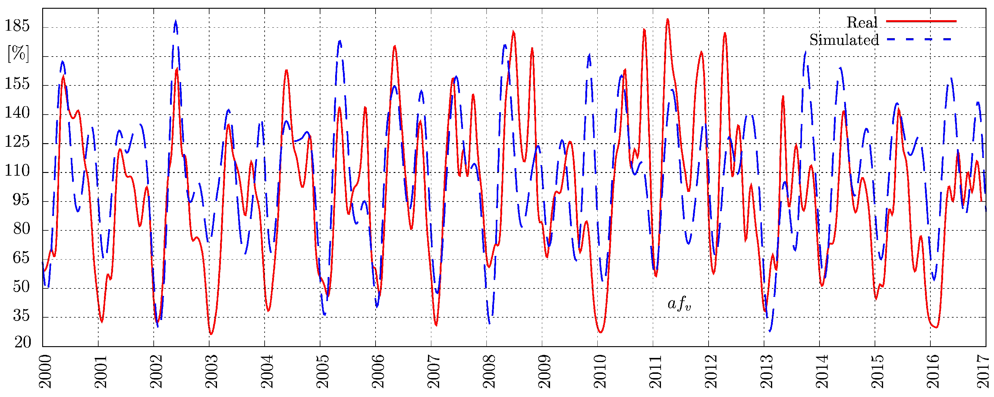
2.3. Hydroelectricity Variability Modeling

The variability of hydroelectricity was thus addressed within the model to account for local weather dynamics. Although Colombia’s weather reflects a periodic behavior pattern throughout the year, pattern variations due to the ENSO phenomenon alter the cyclical behavior of the dry and wet seasons [33,34], increasing or decreasing the water availability of the rivers used to power the hydro plants during La Niña or El Niño events, respectively. The hydroelectricity availability factor ( a f v ), also called (V) availability factor in Figure 5, must thus account for the seasonality and ENSO phenomenon to incorporate more realistic characteristics. The seasonality and ENSO phenomenon were thus modeled using deterministic functions to approximate the water contribution of the Colombian rivers. Documented seasonal variations due to La Niña and El Niño events suggest that these phenomena have been in play since 1950 [35]. In particular, Colombia has been through several periods of risky electricity scarcity due to the appearance of strong El Niño events in 1991/1992, 1997, 2008, and 2015/2016. Prior researchers have documented the strange attractors’ (or chaos) influence on Colombian hydro-climatology [33], confirming to some extent the existence of chaotic deterministic components in the Colombian hydrology.
Historical mean water contributions from 2000 to 2016 obtained from XM (the company that manages the Colombian power market) [32] were analyzed and plotted; the corresponding a f v (in percentage) is shown in Figure 6 by the red line. Note that over the past years the a f v has experienced situations with great potential and also water scarcity. Low a f v values correspond to strong El Niño events.
To model the a f v , the Lorenz chaotic attractor described in Equation (1) was then used to model the ENSO phenomenon, whereas the seasonality was represented by Equation (2). In general, the effects of seasonality are more pronounced when the ENSO appears, i.e., further decreasing water availability in dry seasons and increasing it during wet seasons. Thus, the ENSO and seasonality components were both included in the calculation of a f v . In this sense, we are modeling the seasonality and ENSO phenomenon, as several climate researchers have [33,36,37].
The Lorenz attractor in its mathematical form is defined as [38]
x ˙ = a ( y x ) y ˙ = x ( b z ) y z ˙ = x y c z ,
where a, b, and c are parameters that were tuned for generating chaotic dynamics; and x, y and z are the state variables [38].
The seasonality patterns are represented through Equation (2), obtained from [30].
a f v = 1.01 + 0.47 sin ( 2 π t 0.45 π ) cos ( 2 π t 0.45 π ) + 0.25 sin ( 2 π t 0.55 π )
To incorporate both the ENSO phenomenon and seasonality patterns, these equations were then combined and used to model the a f v .
Finally, the stock-flow structure and the parameter values used to implement this more realistic variability are shown in Figure 7 and Table 1, respectively.
In principle, the initial conditions and parameter values (a, b, and c) of the Lorenz attractor were set to exhibit the classical butterfly effect, since this behavior was found to better represents the ENSO phenomenon, as shown by [33]. Then, one of the three state variables was selected to represent the ENSO phenomenon by considering their individual dynamics; here, z was selected since it exhibited a behavior similar to the real a f v . Finally, the model was then run to obtain the synthetic series, shown in Figure 6 as the dashed blue line. The resulting simulated line was in good agreement with the real data; MAPE = 11.35%.
The simulated a f v was obtained using only a determined and fixed set of initial conditions. However, as the chaos theory states, slight changes in the initial conditions of a chaotic system can result in very different behaviors. The simulated results thus represent only one possible reality of the Colombian a f v , so that by varying the initial conditions of the Lorenz attractor it is possible to obtain many different realities.

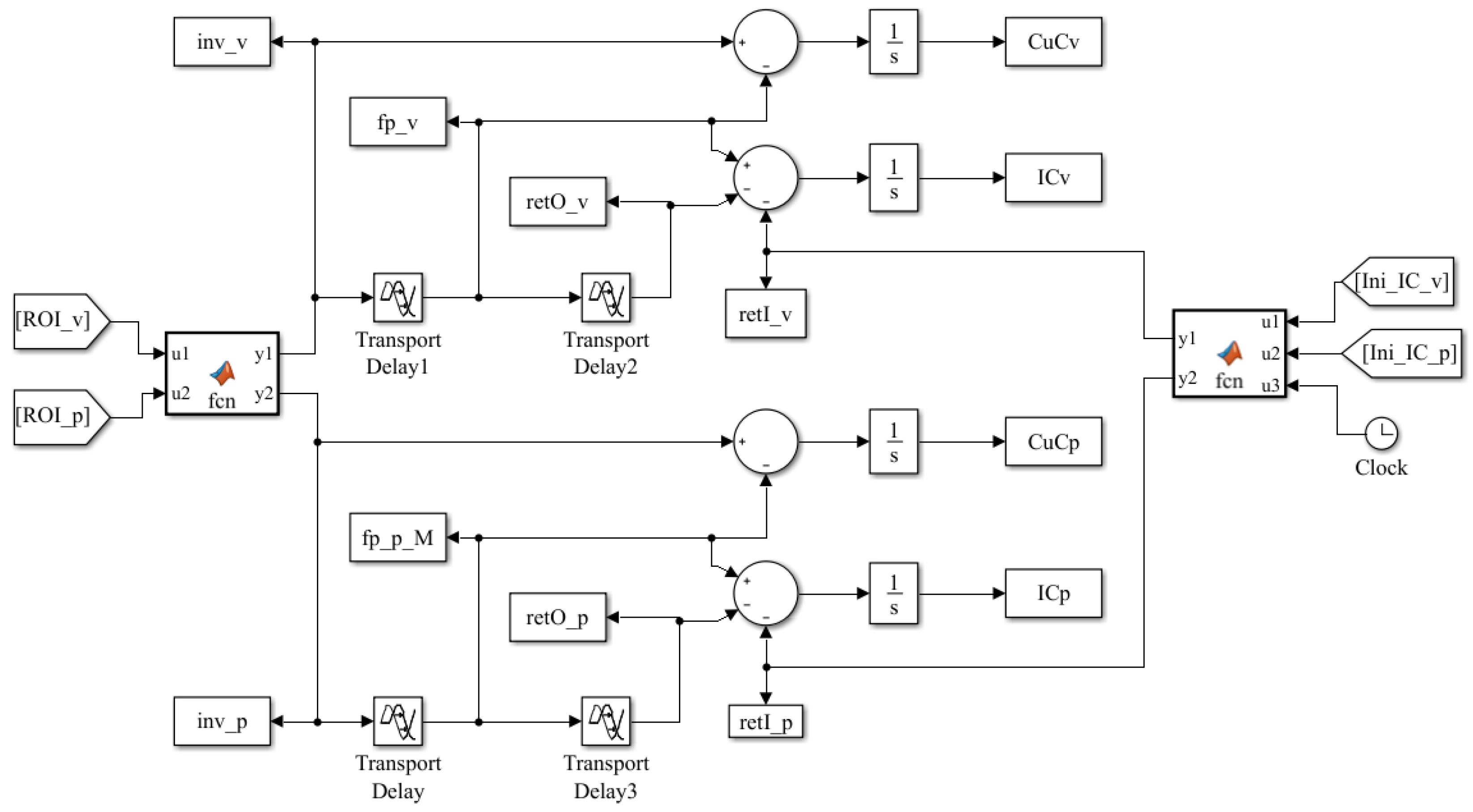
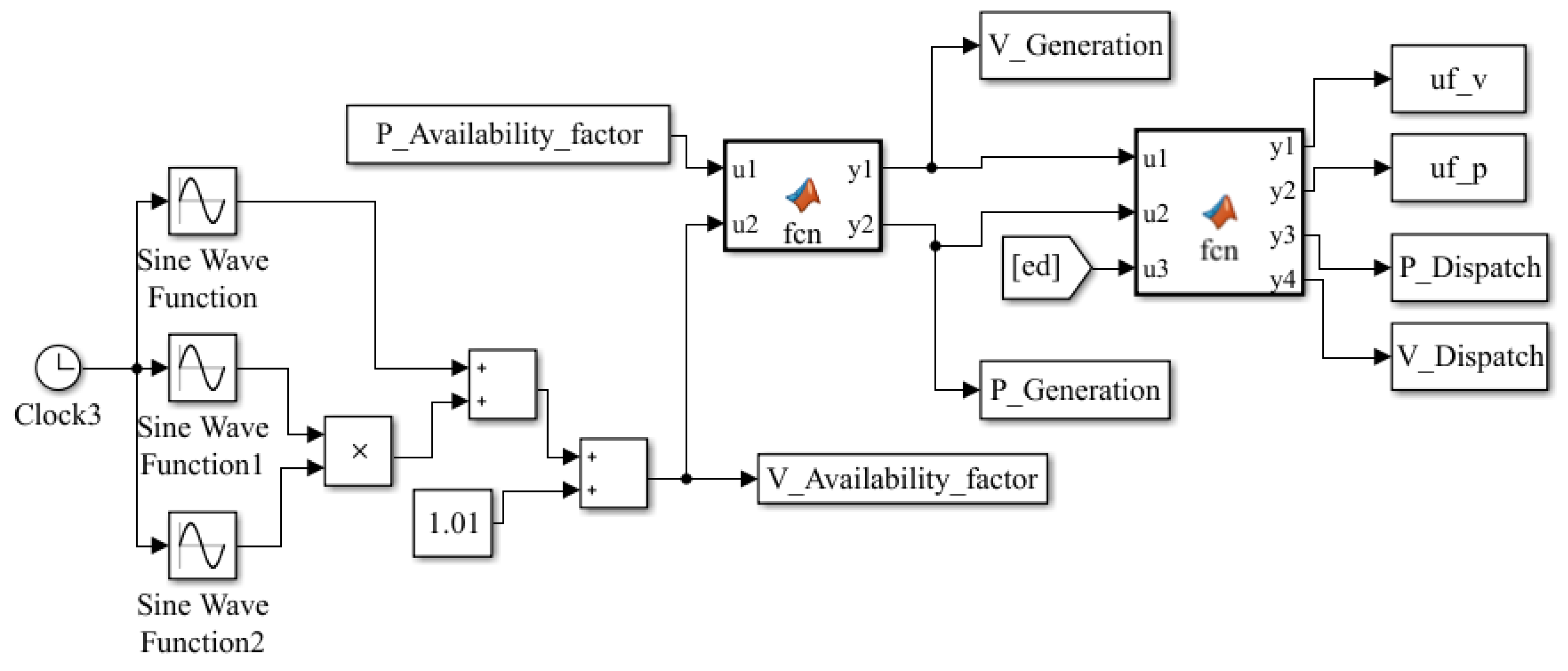
2.4. Block Diagrams of Simulink

To more easily apply DS tools and thus describe in more detail the energy SD model and explore a broader spectrum of scenarios and from different perspectives, the proposed stock-flow structure was then transformed into a Simulink block diagram to investigate the SD model problem. The resulting Simulink block diagrams and dynamic equations are in Appendix A; further details can be found in [13].
The transformation of the stock-flow structure into the Simulink block diagram is intuitive and does not require to program numerical methods for solving ODEs; furthermore, Simulink provides advantages over other S D software packages, such as Vensim, Powersim, and Stella, since an unlimited number of DS tools can be implemented. To transform a stock-flow structure into a Simulink block diagram, it is only necessary to find the SD variable correspondence with the Simulink block variables. When comparing Figure 2, Figure 3, Figure 4, Figure 5 and Figure 7 with Figure A1, Figure A2, Figure A3 and Figure A4, know that the structures are similar and their correspondence should be easy to follow.
Once the SD model has been transformed into Simulink block diagrams, any DS strategy of analysis can be implemented for investigating its dynamics, as we shall see in the following sections. Note that with a Simulink model (i.e., a DS model), D S tools can be implemented or applied in an easier form than having the normal system equations programmed in MATLAB, C++, Python, etc.

3. Modeling the V/P Scenarios

The generation of the V / P scenarios is discussed in this section, now that the hybrid model has been explained in the previous section. In addition, prior to obtaining the simulation results, the proposed model was validated.
Each V / P scenario was simulated for only one initial condition of the Lorenz attractor, i.e., only one possible reality. As discussed above, chaotic attractors are very sensitive to changes in their initial conditions; therefore, any change in the initial conditions of the Lorenz attractor can be seen as a different reality—e.g., asdifferent actions performed by human beings or just general changes of the entire world—any of which can affect the environment or climate, and consequently the a f v . Varying the initial condition of the state variable used to represent the ENSO phenomenon (i.e., z) generates very different synthetic series, each of which can be seen as a different possible reality of the a f v , or as a different scenario of the ENSO phenomenon. However, the question arises as to how many synthetic series should be computed.
To address this question, the variance of one market variable under varying initial conditions can be computed, thereby allowing a clearer picture of how many synthetic series are required to equilibrate the variance. Here, the variance of the unmet electricity demand ( u n m e t e d refers to the electricity that the power system is unable to supply) was calculated under varied condition of z; the results are shown in Figure 8.
Note from Figure 8 that the variance due to varied Lorenz attractor scenarios fluctuated drastically in the first 2000 simulations; however, after 4000 simulations, the variance reached an equilibrium. Despite continued variations to the initial condition of z, the resulting synthetic series did not change significantly. As a result, by simulating the electricity market model up to 4000 times, 4000 different synthetic series or 4000 distinct scenarios of the Colombian electricity market are guaranteed. These 4000 possible realities can be considered for studying different share scenarios of P and V installed capacities.
Currently, the Colombian electricity mix consists of approximately 70% hydroelectricity (i.e., V) and 30% thermal electricity (i.e., P) [29]; however, the share of V will likely continue to grow as the share of P decreases due to concerns regarding the environmental impact of fossil fuels. Still, as many markets worldwide exhibit similar market conditions with different P and V shares, the impacts of scenarios ranging from 0%V/100%P to 100%V/0%P were assessed with their corresponding electricity market performances using DS tools while incorporating the ENSO phenomenon. Thus, this process provides a detailed analysis of the V / P scenarios thanks to the developed DS tools, and an assessment of the electricity market’s performance under more realistic conditions.
Although the studied scenarios are specific to the Colombian electricity market, the main characteristics and properties of the supply and demand rules are followed by many other countries; as a result, the findings can be extended to other countries. In fact, as the ENSO phenomenon affects vast areas of Asian and Pacific regions, this methodology can be applied to several countries. Although the specific technology may vary (e.g., the hydroelectricity usage in Colombia), the general discussion of the variability associated with renewable electricity generation may be applicable.
As discussed above, the initial conditions were varied to generate 4000 synthetic series of a f v , i.e., 4000 distinct scenarios of the ENSO phenomenon impacting the Colombian electricity market. These scenarios were then considered over each studied V / P scenario. Once the 4000 synthetic series were computed for each V / P scenario, the average synthetic series of each key variable of the electricity market was calculated and plotted; results are shown in Section 4.1. As these are averaged values, the output behavior patterns exhibit smooth shapes. Furthermore, the synthetic series were averaged to capture their most frequent behaviors or their central tendencies. Additionally, note that this is not the same as a traditional SD sensitivity analysis because traditionally, (i) the ENSO phenomenon would not be accurately portrayed, (ii) the exact V / P scenario leading to a determined behavior could not be identified, and (iii) simulating only a few scenarios would be possible, considering the limitations of the SD software packages that we have explained before.
As a near-infinite number of V / P scenarios could be simulated, the computational power required must be considered. In our case, 100 V / P scenarios from 0% to 100% in 1% increments, and using only hydroelectricity as the renewable source, were computed. Considering the 4000 synthetic series generated by the Lorenz attractor and the 100 V / P scenarios, this resulted in 400.000 total simulations. This makes our study a vast analysis to a degree that has never been reached before in this area.

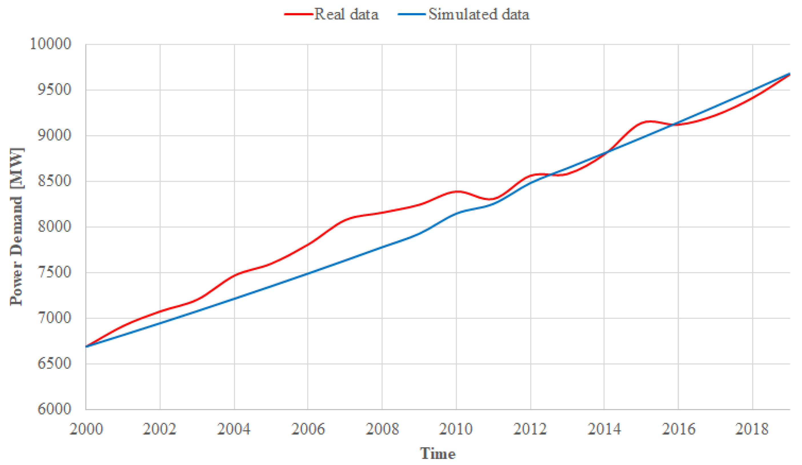
3.1. Model Validation

The complete validation process is out of the scope of the paper and thus not widely discussed here. The model robustness was tested following the method explained in [39,40]; all validation tests were successfully passed. In fact, a more advanced sensitivity analysis was applied, as detailed below.
In addition, basic time series of the proposed model were calculated in Vensim, MATLAB®, and Simulink to verify their accuracy; all showed good agreement (see some examples in Figure 9 and Figure 10). In fact, to verify the accuracy of the proposed model even further, the model was run starting from 2017; the modeled data from 2017 to 2019 were then compared to obtained Colombian electricity market data. Good agreement was found, including during the months of energy crisis that occurred in 2017 and 2019, as shown in Section 4.2 and Section 5.1. During these months, the market was highly impacted by the ENSO phenomenon. Additionally, the model successfully predicted the perturbation in January/February and November/December 2019 caused by the delay of Hidroituango (a 2400 MW hydro plant) announced in April 2018 [41,42,43]. Thus, the model was determined to predict accurately electricity market fluctuations.
While taking all of that validation process into account, the model was analyzed starting from 2020. Hence, the time horizon of the simulations goes from 2020 to 2050, using a daily time step.

3.2. Model Assumptions and Limitations

The start-up time of thermal power plants was not modeled, since its practical implications are negligible in contrast with the time delays associated with the construction and decommissioning of power plants. Subsidies were not considered, as there currently exists no subsidy policy in the Colombian electricity market. Electricity storage was not considered, and fuel prices were kept constant over the 33-year simulation period. Electricity generation technologies were aggregated into two buckets: renewables and fossil fuels (variable and permanent capacities, respectively). Furthermore, here, only hydropower was considered as a renewable electricity source, due to its prevalence in the Colombian market, which is not encouraging the installation of other renewable energy sources. The results of this paper are thus limited to the Colombian case and foreign power markets with similar characteristics.

4. Simulation Results: A Bifurcation Perspective

The bifurcation theory has been broadly used in DS to study the behavior of physical systems against parameter variations [45]. This methodology allows a broad spectrum of behaviors to be obtained and analyzed as a parameter is varied; furthermore, the parameter causing a determined behavior can be identified, thereby remedying a drawback of the sensitivity analysis using SD software packages.
In fact, the sensitivity-based bifurcation analysis is simple to implement once the stock-flow structure has been transformed in a Simulink model. Several authors explained the implementation with great detail in [46,47,48].

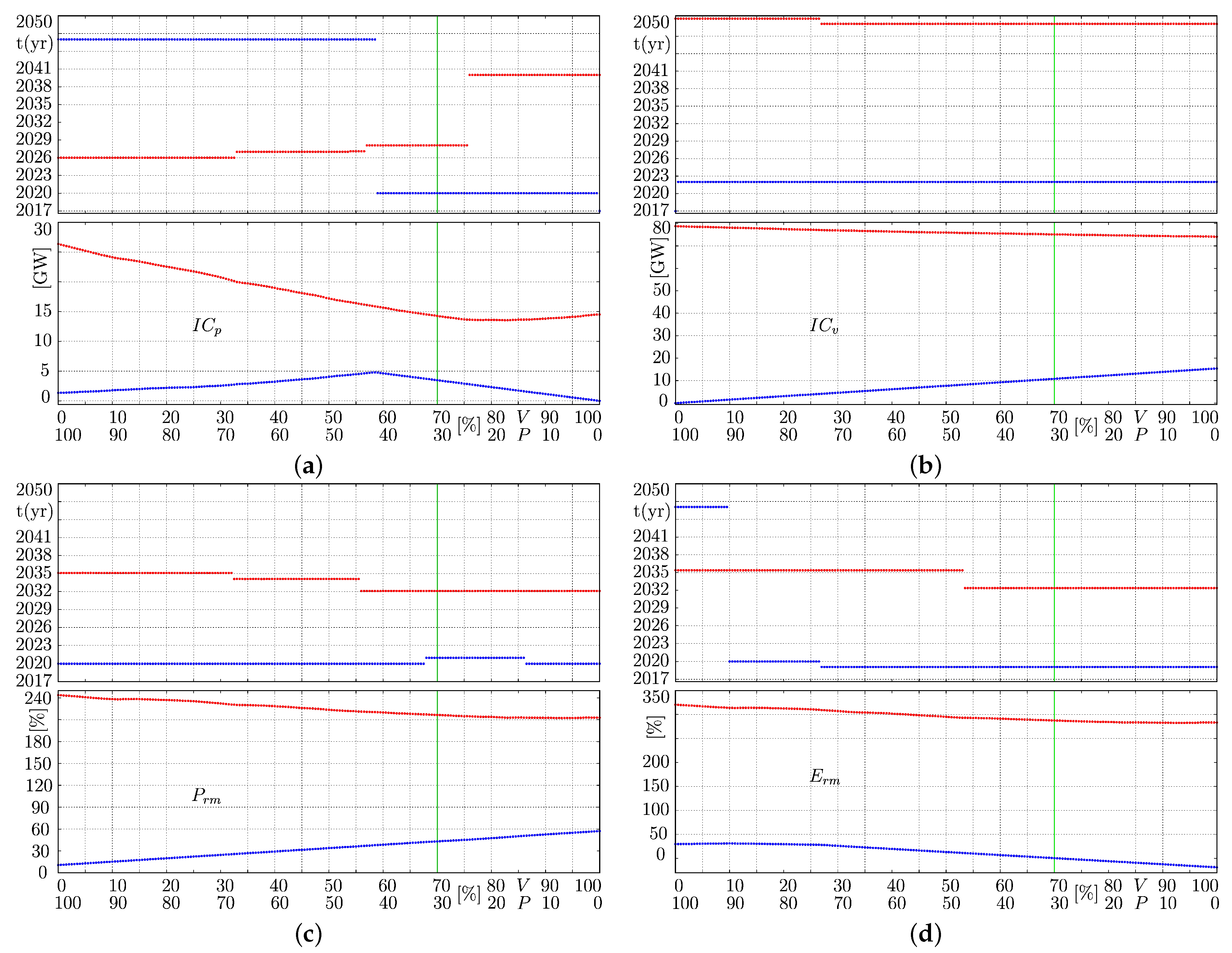
4.1. V/P Installed Capacity Scenarios

Key variables of the electricity market model were thus assessed under the modeled V / P scenarios, while accounting for variability of the ENSO phenomenon using the proposed advanced sensitivity analysis based on bifurcation theory; results are shown in Figure 11, where the upper and lower x-axes represent the installed V and P capacities, respectively. Accordingly, each scenario provides an averaged series containing all possible solutions of the system under each studied market share of varied V and P generation.
The behaviors for the installed P capacity ( I C p ) and installed V capacity ( I C v ) are shown in Figure 11a,b, respectively. Despite the chaotic variability introduced via the ENSO phenomenon, both the I C p and I C v show similar white spaces and behavioral patterns. These white voids reflect the lack of a solution, i.e., discontinuities. However, the I C v demonstrated a more organized pattern, regardless of V / P scenario, and was characterized by rapid, uniform growth. In essence, it appears that the dispatch merit order effect together with environmental and price issues causes a more uniform and organized increase in V capacity; as the electricity demand ( e d ) increases, so does the construction of hydroelectric plants. Conversely, since the I C p is directly dependent on the availability of hydropower, the chaotic component of the ENSO phenomenon is automatically transferred to its dynamics. When the ENSO phenomenon greatly affects the V generation, larger shares of I C p are required to support it. Accordingly, the I C p shows less-organized behavior patterns. Thus, a greater installed V capacity results in a lower installed P capacity. In other words, the market share of P tends to be reduced as the capacity of V increases. However, the I C p could not be reduced below 13 GW under an (80%V, 20%P) scenario. Further increases of I C v might actually cause an increase in the I C p , to support the V technology. Increasing the I C v thus provokes a high degree of variability in the market, which is then mitigated by increasing the I C p . Thus, if Colombian decision makers desire to be as environmentally friendly as possible without sacrificing the security of electricity supply, the best case scenario is (80%V, 20%P). Accordingly, this can also be recommended to electricity markets of other countries that are affected by the ENSO phenomenon. Currently, in Colombia, hydroelectricity plants are being installed as thermal power plants are being decommissioned, suggesting that the market is moving towards this scenario: continued efforts should thus be made to reach (80%V, 20%P), but increasing non-conventional electricity generation should also be continued to complement the high variability of the 80%V technology.
However, Figure 11b shows that as the share of V generation increased (while the P decreased), the overall I C v slightly decreased, rather than remaining constant or increasing. By having a large V capacity installed, the resulting higher degree of variability constrained its overall growth; as a result, less renewable generation capacity was installed over time.
Nevertheless, market dynamics did not allow for a 100% hydroelectricity-dependent market. A significant amount of P capacity was found to be necessary in the electricity mix to guarantee security of supply and reliability. Even the scenarios beginning at either spectral extreme (i.e., (0%V, 100%P) or (100%V, 0%P)) ended up in different combinations of both technologies; still, the V generation deployment occurred more rapidly and to a greater extent than did the P generation, likely due to environmental constraints.
The power reserve margin ( P r m ), detailed in Figure 11c, also presented white empty places due to the direct transference of the discontinuous behavior of the I C p and I C v to the P r m . However, a larger share of V capacity being installed resulted in reduced P r m . As expected, if a larger share of hydropower is used to meet the majority of the e d , the incentives for expanding the P or V capacity are also reduced, as the lower price of hydropower generation discourages system expansion. For this reason, the greater the V capacity installed, the lower the P r m achieved over time. Larger shares of P capacity values thus cause higher values of P r m due to price issues, but also allow scenarios at which the P r m reaches the lowest possible value, due to the differences in the lifetimes and construction times of both technologies. In other words, scenarios with an electricity system dominated by thermal generation have overall shorter lifetimes; considering that the installation of hydropower plants takes, on average, 5 to 7 years before become operational, this leads to a more rapid decrease of the P r m . Conversely, a greater installed hydropower capacity ensures a longer lifetime of the entire system, together with a complementary technology (thermal plants) that can be installed in only 2 or 3 years. This, on the contrary, causes the P r m to decrease slowly.
Similarly, the energy reserve margin ( E r m ) is prone to be reduced as more V capacity is installed, as shown in Figure 11d. Again, increased generation of hydropower means lower revenue for the producers, thereby discouraging the expansion of both P and V capacities. However, this also increases the risk of electricity blackouts. Similarly to the P r m , the E r m tends to exhibit less dangerous values (close to zero or even negative) as the share of hydropower is reduced (which also implies a larger share of thermal generation). This can be explained by the a f v dynamics: a scenario with less hydropower immediately results in a less variable electricity system. Under a high share of P capacity, the E r m attains higher values, and an electricity market with lower probabilities of exhibiting zero or negative values of E r m (rationing events) can be expected. However, this does not necessarily mean that rationing events can be avoided for greater permanent shares, as they were still present, as shown in Figure 11g. At the current Colombian case (70%V, 30%P), the maximum rationing episode was not as high as the one exhibited by the larger shares of V capacity, but was higher than those exhibited by those with lower shares of V capacity. In other words, in terms of unmet electricity demand, the BaU scenario of Colombia is currently close to the ideal scenario (62%V, 38%P); if the V capacity is further increased, the risk of blackouts also increases.
Overall, under scenarios with larger shares of hydropower generation, the thermal producers sold or dispatched less electricity, and vice versa, as shown in Figure 11e. However, once the hydropower capacity shares reached 89%, any further increase in the share did not continue to reduce the thermal electricity dispatched. As explained in the I C p scenarios, a larger share of hydropower provoked a higher degree of variability, which was then mitigated by increasing the capacity of installing P generation plants. Although the dispatch of renewable electricity ( d i s p v ) did increase as the share of renewable capacity increases, an upper confidence limit (around 19 TWh) was always hit, regardless of V / P scenario, as shown in Figure 11f. This is explained by the fact that at the end of the simulation, only hydropower generation was able to meet the total e d ; as a result, its maximum value achieved met the final amount of e d required.
The unmet e d ( u n m e t e d ), shown in Figure 11g, was nonzero in all V / P scenarios, due to the model’s basis of the Colombian market, in which there exist grid problems and unplanned maintenance for power plants in several regions of the country. The u n m e t e d did reach low values for V / P scenarios within (0%V, 100%P)–(62%V, 38%P). However, for the remaining V / P scenarios, the u n m e t e d reached higher values. Accordingly, an ideal best V / P scenario would thus be (62%V, 38%P) to avoid high u n m e t e d and any severe rationing events. A greater share of P capacity might lead to a higher u n m e t e d ; by having a higher share of P generation, the capacity is reduced more quickly for environmental reasons, leading to higher u n m e t e d events. Likewise, larger shares of V capacity (above 63%) increase the risk of presenting critical values of u n m e t e d , due to variability issues. Accordingly, further increases of the current hydropower capacity in Colombia might subject the market to more critical rationing events. In the next section, the expected time of occurrence of these situations is detailed.
Lower market prices ( m p ) were observed for greater shares of P capacity, as shown in Figure 11h. At these share distributions, there is less risk of u n m e t e d events; the rationing price ( R A P ) tariff is thus lower, allowing consumers a more competitive m p . If the share of V generation is increased above 70%, consumers might be forced to pay higher electricity prices at some time during the 33 years of simulation; when this may occur is discussed in more detail in Section 4.2. So far policy makers and energy investors know that there exist near-ideal combinations of P and V capacities of 35% and 65%, respectively. Further increases or decreases in V generation might increase the risk of electricity blackouts, especially if increased over 65%.

4.2. Confidence Limits and Their Occurrence

The proposed DS methodology is a derivation of the bifurcation method, as explained in Section 4. The method allows more information to be obtained from the bifurcation sensitivity analysis, especially the maximum and minimum values of the system behavior for each parameter ( V / P scenario) with its corresponding year of occurrence.
The DS tools were thus used to obtain further information from the proposed SD model and provide an in-depth V / P scenario analysis. The corresponding confidence limits of the advanced sensitivity analysis of the results shown in Figure 11, together with their exact year of occurrence, are shown in Figure 12 and Figure 13.
As seen in Figure 12a, scenarios containing greater shares of P capacity are expected to reach their lowest I C p in approximately 2046, suggesting that the P component of the electricity matrix may disappear by 2050. These scenarios reached a maximum I C p around 2028. This is because the critical values of the E r m are expected to occur in the short-term (around 2020), as shown in Figure 12d, which incentivizes the capacity expansion of both V and P components; as a result, a maximum value of I C p is met in the mid-term. The V / P scenarios within the range (58%V, 42%P)–(75%V, 25%P), including the current Colombian case, experienced the lowest value of the I C p near 2020, whereas the maximum value was met near 2029, due to the short-term critical values of the E r m . Thus, electricity markets in these scenarios might also expect significant reductions of their thermal components in 33 years. However, further increasing the V capacity would cause, after an immediate reduction of the I C p , an increased I C p over the next 20 years due to the high degree of variability introduced in the system. Thus, the increased thermal capacity might be part of the electricity matrix for many more years.
Due to the decommissioning and depreciation of old hydropower plants, the lowest I C v values were reached near 2022, whereas the highest values were reached near 2050, as shown in Figure 12b. Thus, regardless of V / P scenario, the market share of renewables will drastically increase after 2022. This dynamic will not happen before 2022 because of the construction time (delay time); regardless of scenario, the installation of renewable plants takes time. While this occurs, the existing renewable capacity will become obsolete; as a result, around 2022 (just before a new renewable plant enters the market) the lowest renewable capacity should be achieved. In general, renewable electricity is expected to continue growing in the short, middle, and long-term future due to environmental concerns.
Due to the continued reduction of the I C p and the natural decommission and depreciation of hydropower plants, the P r m reached its minimum near 2020 in all V / P scenarios, as shown in Figure 12c. The continuous investments in both thermal and hydropower capacity aimed at overcoming the critical situations of 2020 then caused a maximum P r m near 2035 or 2032. The P r m was not affected by the ENSO phenomenon, as it is defined only by the I C p and I C v .
By considering the impact of the ENSO phenomenon, the E r m experienced critical situations around 2020 in most V / P scenarios studied, as shown in Figure 12d; only scenarios using fossil fuel shares greater than 91% avoided this critical situation (a zero or below-zero value). In other words, only the variability of renewable scenarios with 1–9% renewables can be mitigated by the corresponding 91–100% fossil fuel capacities. All studied V / P scenarios encountered a maximum E r m near 2033, due to the continuous investments in both thermal and hydropower capacity to overcome the critical situations of 2020. Thus, regardless of increases or decreases in the share of renewable electricity, the Colombian market will likely experience a serious electricity risk ( E r m near zero) in the short term.
According to the behavior of the confidence limits’ times of occurrence d i s p v shown in Figure 13b, the minimum d i s p v values shall be reached in the short-term, as they are related to the minimum values of the I C v , whereas the maximum values shall be met in the distant future, as high e d yields high hydroelectricity consumption. Within the V / P range (0%V, 100%P)–(46%V, 54%P), dispatch of fossil-generated electricity ( d i s p p ) reached a minimum value of near-zero close to 2026 (see Figure 13a), as the hydropower generation can meet the total e d . Although these scenarios were characterized by initial domination of the electricity matrix by thermal generation, hydropower generation was later highly deployed. Thus, under these scenarios, the thermal component reached a maximum d i s p p near 2021. However, in the scenarios involving V / P ranges of (47%V, 53%P)–(87%V, 13%P) the hydropower plants met the total e d sooner, since the shares of the V capacity were larger. The lowest d i s p p values thus took place around 2020/2021, whereas the highest d i s p p values occurred shortly afterwards, around 2022, when the variability and small installed hydropower capacity (due to the decommissioning of old plants) affected the electricity production of the hydropower plants. Within the V / P range (88%V, 12%P)–(100%V, 0%P), d i s p reached a maximum around 2024, because the hydropower generation was still not well developed enough to meet a large proportion of the demand.
In the scenarios involving the V / P ranges of (0%V, 100%P)–(62%V, 38%P), less electricity rationing (i.e., lower u n m e t e d ) was found than in those involving greater capacities of installed hydropower (see Figure 13c). Although rationing events were avoided in the short-term, most scenarios saw rationing by about 2045. Electricity markets comprised of V / P scenarios within (63%V, 37%P)–(100%V, 0%P), including that of Colombia, however, experienced u n m e t e d around 2020/2021.
When a greater share of P capacity was installed, the minimum and maximum values of the m p occurred further apart, with the minimums occurring in the short-term and maximums occurring in the long-term, as shown in Figure 13d. The lowest prices occurred near 2026 due to the combination of thermal and hydropower generation, which set competitive prices for consumers. The subsequent decreases of thermal capacity and P r m / E r m as a consequence led to a higher m p to incentivize capacity expansion. However, when the share of the V generation was further increased, m p reached its minimum and maximum values at almost the same time, close to 2020. This was due to the rationing events appearing near to this timeframe in these scenarios, which was preceded by hydropower meeting most of the e d and setting a very low tariff. Once the critical rationing situations appeared, the m p increased to incentivize capacity expansion. Overall, a greater share of V generation leads to a higher m p . Together, these results will be useful for decision makers in Colombia, including investors and policy makers. Without additional inputs, such as complimentary renewable sources, storage technologies, or subsidy policies, increasing the renewable generation will likely affect the market price in the short-term and middle-term.

5. Simulation Results: A Control Theory Perspective

An algorithm inspired by the input–output relationship diagram used to design nonlinear controllers [26] was then developed to illustrate in detail the rationing scenarios undergone by the proposed electricity market model. The resulting 3D diagram maps each possible rationing scenario with its corresponding date (year and month) and probability of occurrence.

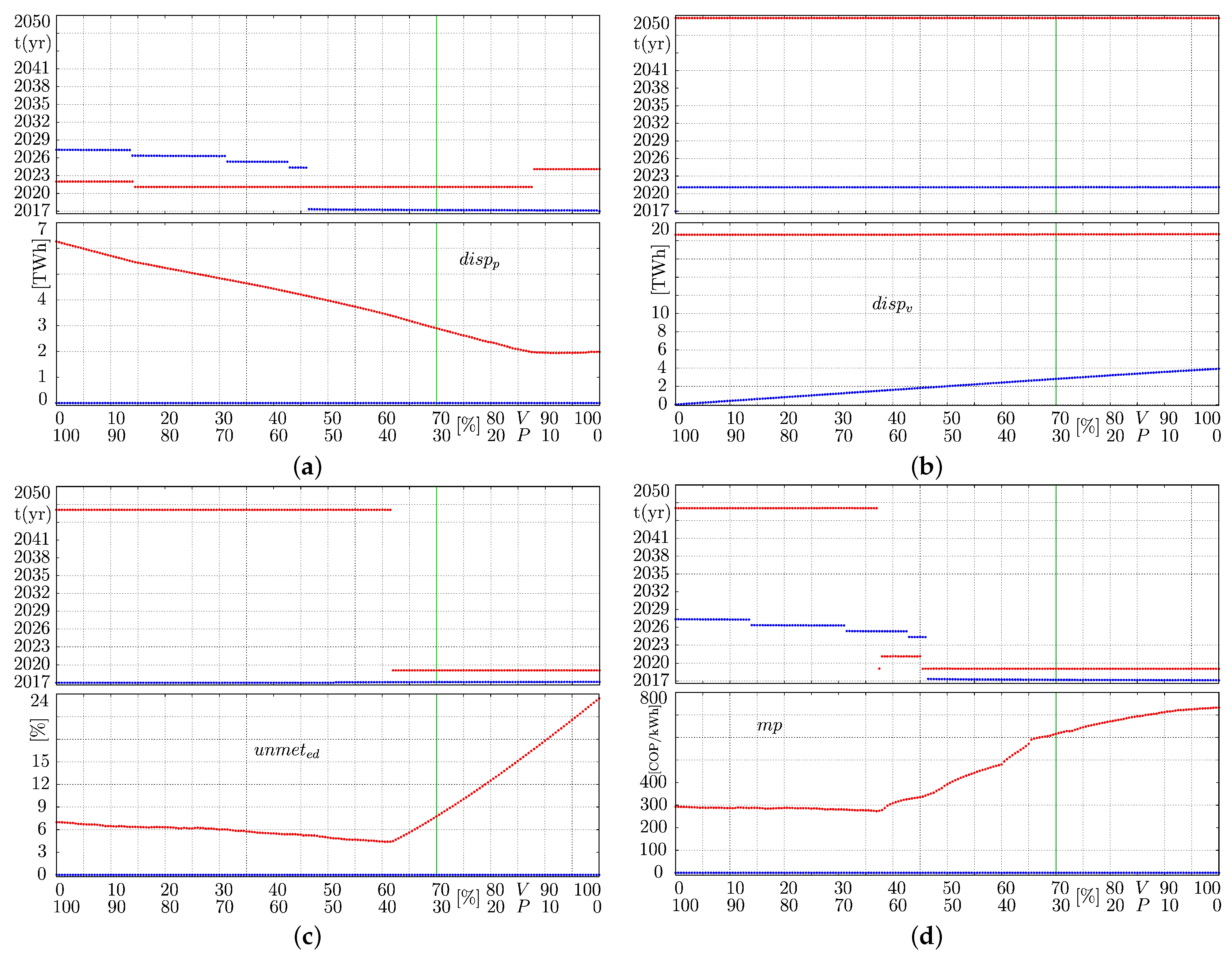
5.1. Detailed Rationing Events

To clarify the u n m e t e d events exhibited by the proposed electricity market model, the input–output relationship diagram derived from control theory [26] was used to estimate the date (year and month), duration, and probability of occurrence of each electricity blackout.
The resulting input–output relationship diagram computed for each V / P scenario is shown in Figure 14. Here, the bottom-left diagram illustrates the frequency of rationing months ( F R M ) for each V / P scenario; the upper-left and right diagrams estimate their corresponding years and months of occurrence, respectively; and the bottom-right diagram shows the probability of occurrence of each rationing episode in 3D.
In the Colombian case (marked by the horizontal green line), six months of electricity rationing was expected over the 33-year period studied. According to the upper left diagram, these months are likely to be in 2021, 2046, 2048, and 2049; however, considering that other V / P scenarios overlap with the Colombian case (also undergo six rationing months), the distribution of the six months over these years cannot be certain. It might be three months in 2021 and three more in 2048; it also depends on the months graph. Note that 2021 underwent three rationing months, as did 2048. Still, these results indicate that steps should be taken to mitigate possible rationing in the short-term (2020–2022) and in the long-term (2046–2050 at least), especially given that several critical alerts and much uncertainty were present over the past few years (i.e., 2017 and 2019); more critical electricity issues are predicted to occur.
In the Colombian case, given the corresponding upper-right diagram, these six rationing months are likely to be distributed across November–February, i.e., the dry season: this is likely due to the added stress of the appearance of the ENSO phenomenon. The probability of occurrence even within these months and years varies drastically; still, January of 2021 and 2048 were predicted to be the most dangerous months with probabilities of rationing near 50% and 97%, respectively, as shown in the bottom-right diagram. Steps should thus be taken to mitigate possible rationing in the target areas.
Rather, more stable V / P scenarios were found within the range (0%V, 100%P)–(45%V, 55%P), where only two rationing months were expected in January of 2048 and 2049, with respective probabilities of 97% and 60%. In general, larger shares of P generation lead to more robust security of electricity supply in the short-term and middle-term, and are subject to rationing events only in the long term.
Variable generation greater than 50% increases the risk of rationing events (>3 F R M ), most likely to occur in January, February, July, November, and/or December. Even when a large share of P technology is initially installed, V generation overtakes P generation over time (due to environmental and price issues), thereby compromising the security of supply of the long-term. A larger share of P generation may be more advantageous in the short-term and mid-term, but is unfavorable to the environment. Either way, rationing events are more likely to occur in the long-term than those in the short-term. In particular, January 2048 appears to be the most dangerous episode, with a probability of nearly 90%. Due to the Colombian climate and the ENSO phenomenon, December–February is the most risky time of year; decision makers should thus develop new strategies moving forward, especially for these critical months.

5.2. Leverage Points

To study the general leverage points of all V / P scenarios, an algorithm was developed to detect the final shares (i.e., in 2050) of P ( I C p ) and V ( I C v ) generation for each V / P scenario, thereby aiming to find out if different mixes of electricity sources lead to specific leverage points (final V / P combination) over time.
The resulting leverage points are illustrated in Figure 15. Regardless of the initial V / P scenario, the Colombian market is expected to evolve to approximately (90%V, 10%P). Accordingly, regardless of the initial V / P installed capacity scenario of any country, renewable generation (here, hydropower) will become much more dominant by 2050 (see Figure 15a). Colombia and other countries with similar power markets should thus expect their electricity markets to evolve over the next 33 years to support nearly 90% of their electricity production from renewable technologies, and nearly 10% of their electricity production from nonrenewable technologies (see Figure 15b). This result is incentivized for environmental reasons and the merit order effect, which several power markets worldwide share with the Colombian case.
These results indicate that the Colombian government and energy authorities of countries with similar power markets should recognize that many energy systems are evolving towards an electricity market comprised of 10% nonrenewable (see Figure 15b) and 90% renewable (see Figure 15a) sources.

6. Conclusions

In this work, renewable capacity scenarios of the Colombian power market were investigated in order to analyze, determine, and anticipate desirable and undesirable behaviors. This process was carried out under a hybrid modeling scheme, combining two methodologies. The proposed model was first derived using SD methodology [27], and then transformed into a DS model by converting the stock-flow structure into a Simulink block diagram. As a result, DS tools could easily be implemented to obtain deeper and more detailed insights and to discover counterintuitive behaviors.
The resulting combined methodology will enable researchers using SD methods to increase the impact of their results and enrich their analysis, whether using the bifurcation and control theory tools developed here, or any other number of applicable DS tools. Indeed, the broader scenarios that can be investigated and the insights that can be obtained (very detailed and from different perspectives) will be exploited by policymakers to develop a deep understanding of the electricity markets’ dynamics and to make better decisions. For instance, now policymakers know how the variability of the renewable generation will affect the Colombian power market in the short-term and long-term; they know that new and diversified means need to be installed as soon as possible to avoid electricity blackouts; and they know it is inevitable that Colombia and other countries with similar market conditions will achieve an energy mix of nearly 90% renewable and 10% nonrenewable sources in the long-term, so they need to find a way to counteract the huge variability associated with this large share of renewable capacity that will be injected to the electricity system.
The resulting SD/DS study indicated that an installed capacity share of (80%V, 20%P) will reduce C O 2 emissions. However, further modification to the I C v causes a market response increasing the share of nonrenewable sources: increasing the I C v causes a high degree of variability, thereby incentivizing the expansion of P generation to guarantee the supply of electricity, whereas decreasing the I C v causes short-term expansion of P generation to meet the e d and guarantee the supply.
Once an (80%V, 20%P) scenario is achieved, this market share should be maintained and only increased by non-conventional generation sources if the goal is to achieve an environmentally friendly scheme; installing a larger share of variable (renewable) generation will cause a higher degree of variability in the market, resulting in lower usage of the renewable capacity and an increase in the capacity of nonrenewable sources. A greater share of permanent capacity will lead to less dangerous values (close to zero) of E r m . Basically, in this scenario (high shares of permanent capacity) the electricity markets get rid of the variability problem. Overall, the V / P scenario of (62%V, 38%P) appears to be the best case for reaching the lowest u n m e t e d value.
Electricity markets with V / P scenarios within the range (0%V, 100%P)–(75%V, 25%P), including the Colombian case, are expected to eliminate or significantly reduce their nonrenewable components by 2050. However, short-term increases of the variable contribution beyond 75% will have the opposite effect, causing a market response of an increase in the thermal plants that continue generating electricity even beyond 2050.
Overall, power markets containing larger shares of variable generation might expect to have more critical rationing events (i.e., blackouts). Accordingly, it is recommended that Colombia maintains its current hydropower capacity and diversifies its electricity matrix by incentivizing non-conventional technologies that were out of the scope of this work, such as solar or wind power. As is, lower consumer electricity prices are obtained by installing less variable capacity and more nonrenewable capacity; larger shares of hydroelectricity may produce higher risks of blackouts, leading to increases in the m p .
This study also revealed that Colombia is under serious risk of short-term electricity scarcity, and also may required several rationing events during the 33 years we simulated, especially in 2021/2022, 2048, and 2049. Not only will the delay of Hidroituango stress the electricity system; the progressive installation of renewables will increase the system’s variability, and the rapid decommissioning of fossil fuel power plants will reduce the renewables’ support. To prepare for the short-term future, new capacity must be installed as soon as possible to diminish the risk of blackouts. This new capacity needs to be diversified in order reduced the variability associated with the renewable generation. Only supplying with renewables is not enough profitable to promote the installation of other generation sources; the government should incentivize this diversification.
Regardless of initial V / P scenario, renewable technologies are expected to comprise a more dominant share of the markets in the long-term due to environmental concerns, until an equilibrium point of approximately 90%V and 10%P is reached.
The results here explained are only applicable to the Colombian electricity market and other foreign power markets that follow its same rules, and supply and demand laws.

Author Contributions

Conceptualization, J.D.M. and C.J.F.; methodology, J.D.M. and F.A.; investigation, J.D.M. and F.A.; validation, J.D.M. and C.J.F.; formal analysis, J.D.M. and F.A.; writing—original draft preparation, J.D.M., F.A., and C.J.F.; writing—review and editing, J.D.M. and F.A.; visualization, J.D.M.; supervision, F.A. and C.J.F.; project administration, F.A.; funding acquisition, J.D.M. and F.A. All authors have read and agreed on the published version of the manuscript.

Funding

This research was funded by Colciencias under Convocatoria 811 de 2018—Postdoctorados Nacionales, and Dirección de Investigación y Extensión of Universidad Nacional de Colombia—Sede Manizales.

Institutional Review Board Statement

Not applicable.

Informed Consent Statement

Not applicable.

Data Availability Statement

Not applicable.

Acknowledgments

The authors want to thank Universidad de Monterrey for its support.

Conflicts of Interest

The authors declare no conflict of interest.

Abbreviations

The following abbreviations are used in this manuscript:
ENSOEl Niño-Southern Oscillation
SDSystem Dynamics
DSDynamic Systems
FRMFrequency of rationing months
V/PVariable and permanent generation

Appendix A

Appendix A.1. Simulink Block Diagrams

Figure A1. Supply side from (P) and (V) generation. Reprinted with the permission of Reference [13]. Copyright 2018 Elsevier.
Mathematics 09 01560 g0a1
Figure A2. Demand component. Reprinted with the permission of Reference [13]. Copyright 2018 Elsevier.
Mathematics 09 01560 g0a2
Figure A3. Electricity dispatch. Reprinted with the permission of Reference [13]. Copyright 2018 Elsevier.
Mathematics 09 01560 g0a3
Figure A4. Availability factor of the variable generation a f v [14].
Mathematics 09 01560 g0a4

Appendix A.2. System Equations

C u C p = C u C p ( 0 ) + 0 t i n v p f p p · d t I C p = I C p ( 0 ) + 0 t f p p r o p p r i p p · d t C u C v = C u C v ( 0 ) + 0 t i n v v f p v · d t I C v = I C v ( 0 ) + 0 t f p v r o p v r i p v · d t P D = P D ( 0 ) + 0 t d c · d t
i n v p = 0 P D P D ( 0 ) k 1 δ ( t ) P D P D ( 0 ) k 2 δ ( t ) R O I p 0 0 < R O I p 10 R O I p > 10 i n v v = 0 P D P D ( 0 ) k 1 δ ( t ) P D P D ( 0 ) k 2 δ ( t ) R O I v 0 0 < R O I v 10 R O I v > 10
f p p = i n v p ( t C T p ) f p v = i n v v ( t C T v ) r o p p = f p p ( t L T p ) r o p v = f p v ( t L T v )
r i p p = I C p ( 0 ) / L T p ; 0 t 2017 + L T p o t h e r c a s e r i p v = I C v ( 0 ) / L T v ; 0 t 2017 + L T v o t h e r c a s e
R O I p ( t ) = ( m p · u f p V C p V F C p + I p ) V F C p + V C p 100 % R O I v ( t ) = ( m p · u f v V C v V F C v + I v ) V F C v + V C v 100 %
d c = G R D × e p d × P D e p d = 1 ; m p / d m p ε ; d m p = 0 o t h e r c a s e d m p = m p ( t 0.25 ) m p = P v ; P p ; R A P ; ( g e n v e d r m > 0 ) ( g e n v < e d g e n p 0 r m > 0 ) g e n v < e d r m > 0 g e n p > 0 ( g e n v e d r m 0 ) ( g e n v < e d r m 0 )
u f p = 0 ; d i s p p / g e n p ; g e n p = 0 o t h e r c a s e ; u f v = 0 ; d i s p v / g e n v ; g e n v = 0 o t h e r c a s e
d i s p p = 0 ; e d g e n v ; g e n p ; g e n v e d g e n p + g e n v e d o t h e r c a s e ; d i s p v = e d ; g e n v ; g e n v e d g e n v < e d
P r m = ( I C p + I C v ) P D / P D 100 % ; E r m = ( g e n p + g e n v ) e d / e d 100 %
g e n p = I C p · A F p · 30 · 24 ; g e n v = I C v · a f v · 30 · 24 ; e d = P D · 0.7685 · 30 · 24

Appendix A.3. Parameter Values

Table A1. Parameters used in the model based on the Colombian electricity sector [13,14].
ParameterValue
Construction time ( C T )5 yr
Lifetime ( L T )30 yr
Growth rate of demand ( G R D )0.039
Variable cost ( V C )150 COP/kWh
Incentives (I)0 COP/kWh
Variability fixed cost ( V F C )60 COP/kWh
y ( 0 ) 15,521 MW
z ( 0 ) 9320 MW
x ( 0 ) 0 MW
Minimum price ( M P )35 COP/kWh
Maximum increase of price ( M I P )350 COP/kWh
Elasticity of demand ( ε )−0.3

References

  1. Teufel, F.; Miller, M.; Genoese, M.; Fichtner, W. Review of System Dynamics Models for Electricity Market Simulations; Working Paper Series in Production and Energy; KIT: Karlsruhe Germany, 2013; Volume 2. [Google Scholar]
  2. Papachristos, G.; Struben, J. System dynamics methodology and research. In Modelling Transitions: Virtues, Vices, Visions of the Future; Routledge: London, UK, 2019; p. 119. [Google Scholar]
  3. Zapata, S.; Castaneda, M.; Franco, C.J.; Dyner, I. Clean and secure power supply: A system dynamics based appraisal. Energy Policy 2019, 131, 9–21. [Google Scholar] [CrossRef]
  4. Kosai, S. Dynamic vulnerability in standalone hybrid renewable energy system. Energy Convers. Manag. 2019, 180, 258–268. [Google Scholar] [CrossRef]
  5. Asere, L.; Blumberga, A. Government and municipality owned building energy efficiency system dynamics modelling. Energy Procedia 2015, 72, 180–187. [Google Scholar] [CrossRef] [Green Version]
  6. Liu, D.; Xiao, B. Can China achieve its carbon emission peaking? A scenario analysis based on STIRPAT and system dynamics model. Ecol. Indic. 2018, 93, 647–657. [Google Scholar] [CrossRef]
  7. York, R.; Bell, S.E. Energy transitions or additions?: Why a transition from fossil fuels requires more than the growth of renewable energy. Energy Res. Soc. Sci. 2019, 51, 40–43. [Google Scholar] [CrossRef]
  8. Zapata, S.; Castaneda, M.; Jimenez, M.; Aristizabal, A.J.; Franco, C.J.; Dyner, I. Long-term effects of 100% renewable generation on the Colombian power market. Sustain. Energy Technol. Assess. 2018, 30, 183–191. [Google Scholar] [CrossRef]
  9. Cardenas, L.M.; Franco, C.J.; Dyner, I. Assessing emissions-mitigation energy policy under integrated supply and demand analysis: The Colombian case. J. Clean. Prod. 2016, 112 Pt 5, 3759–3773. [Google Scholar] [CrossRef]
  10. Astegiano, P.; Fermi, F.; Martino, A. Investigating the impact of e-bikes on modal share and greenhouse emissions: A system dynamic approach. Transp. Res. Procedia 2019, 37, 163–170. [Google Scholar] [CrossRef]
  11. Wang, J.; Wu, J.; Che, Y. Agent and system dynamics-based hybrid modeling and simulation for multilateral bidding in electricity market. Energy 2019, 180, 444–456. [Google Scholar] [CrossRef]
  12. Ahmad, S.; Tahar, R.M.; Muhammad-Sukki, F.; Munir, A.B.; Rahim, R.A. Application of system dynamics approach in electricity sector modelling: A review. Renew. Sustain. Energy Rev. 2016, 56, 29–37. [Google Scholar] [CrossRef]
  13. Morcillo, J.D.; Franco, C.J.; Angulo, F. Simulation of demand growth scenarios in the Colombian electricity market: An integration of system dynamics and dynamic systems. Appl. Energy 2018, 216, 504–520. [Google Scholar] [CrossRef]
  14. Morcillo, J.D.; Angulo, F.; Franco, C.J. Analyzing the hydroelectricity variability on power markets from a system dynamics and dynamic systems perspective: Seasonality and ENSO phenomenon. Energies 2020, 13, 2381. [Google Scholar] [CrossRef]
  15. Aracil, J. Structural stability of low-order system dynamics models. Int. J. Syst. Sci. 1981, 12, 423–441. [Google Scholar] [CrossRef]
  16. Mosekilde, E.; Aracil, J.; Allen, P.M. Instabilities and chaos in nonlinear dynamic systems. Syst. Dyn. Rev. 1988, 4, 14–55. [Google Scholar] [CrossRef]
  17. Thomsen, J.S.; Mosekilde, E.; Sterman, J.D. Hyperchaotic phenomena in dynamic decision making. In Complexity, Chaos, and Biological Evolution; Springer: Berlin/Heidelberg, Germany, 1991; pp. 397–420. [Google Scholar]
  18. Sterman, J.D. Deterministic chaos in models of human behavior: Methodological issues and experimental results. Syst. Dyn. Rev. 1988, 4, 148–178. [Google Scholar] [CrossRef] [Green Version]
  19. Aracil, J. On the qualitative properties in system dynamics models. Eur. J. Econ. Soc. Syst. 1999, 13, 1–18. [Google Scholar] [CrossRef]
  20. Valencia, J.; Olivar, G.; Franco, C.J.; Dyner, I. Qualitative Analysis of Climate Seasonality Effects in a Model of National Electricity Market. In Analysis, Modelling, Optimization, and Numerical Techniques; Springer: Berlin/Heidelberg, Germany, 2015; pp. 349–362. [Google Scholar]
  21. Redondo, J.; Ibarra-Vega, D.; Becerra-Fernandez, M.; Olivar-Tost, G. Making decisions in national energy markets with bifurcation analysis. J. Phys. Conf. Ser. 2019, 1414, 012008. [Google Scholar] [CrossRef] [Green Version]
  22. Dimitrovski, A.; Ford, A.; Tomsovic, K. An interdisciplinary approach to long-term modelling for power system expansion. Int. J. Crit. Infrastruct. 2006, 3, 235–264. [Google Scholar] [CrossRef]
  23. Heard, B.; Brook, B.; Wigley, T.; Bradshaw, C. Burden of proof: A comprehensive review of the feasibility of 100% renewable-electricity systems. Renew. Sustain. Energy Rev. 2017, 76, 1122–1133. [Google Scholar] [CrossRef]
  24. Shariatzadeh, F.; Mandal, P.; Srivastava, A.K. Demand response for sustainable energy systems: A review, application and implementation strategy. Renew. Sustain. Energy Rev. 2015, 45, 343–350. [Google Scholar] [CrossRef]
  25. Kuznetsov, Y.A. Elements of Applied Bifurcation Theory; Springer Science & Business Media: Berlin/Heidelberg, Germany, 2013; Volume 112. [Google Scholar]
  26. Vander Velde, W.E. Multiple-Input Describing Functions and Nonlinear System Design; McGraw-Hill: New York, NY, USA, 1968. [Google Scholar]
  27. Sterman, J.D. Business Dynamics: Systems Thinking and Modeling for a Complex World; Irwin/McGraw-Hill: Boston, MA, USA, 2000; p. 1008. [Google Scholar] [CrossRef]
  28. Dyner, I. Energy modelling platforms for policy and strategy support. J. Oper. Res. Soc. 2000, 51, 136–144. [Google Scholar] [CrossRef]
  29. XM. Información Inteligente. 2021. Available online: http://informacioninteligente10.xm.com.co/pages/default.aspx (accessed on 10 January 2021).
  30. Morcillo, J.D.; Franco, C.J.; Angulo, F. Delays in electricity market models. Energy Strategy Rev. 2017, 16, 24–32. [Google Scholar] [CrossRef]
  31. Espinosa, O.; Vaca, P.; Ávila, R. Elasticidades de demanda por electricidad e impactos macroeconómicos del precio de la energía eléctrica en Colombia. Rev. MÉtodos Cuantitativos Para Econ. Empresa 2013, 16, 216–249. [Google Scholar]
  32. XM. Información Inteligente. 2021. Available online: http://informacioninteligente10.xm.com.co/hidrologia/Paginas/HistoricoHidrologia.aspx (accessed on 10 January 2021).
  33. Jaramillo, G.P. ¿Atractores extraños (caos) en la hidro-climatología de Colombia? Rev. Acad. Colomb. Cienc 1997, 21, 431–444. [Google Scholar]
  34. Tziperman, E.; Stone, L.; Cane, M.A.; Jarosh, H. El Niño Chaos: Overlapping of Resonances Between the Seasonal Cycle and the Pacific Ocean-Atmosphere Oscillator. Science 1994, 264, 72–74. [Google Scholar] [CrossRef] [Green Version]
  35. XM. Oferta y Generación. Índice Multivariado ENSO. 2021. Available online: http://informesanuales.xm.com.co/2013/SitePages/operacion/2-9-Anex-Indice-multivariado-ENSO.aspx (accessed on 10 January 2021).
  36. Vallis, G.K. El Niño: A chaotic dynamical system? Science 1986, 232, 243–245. [Google Scholar] [CrossRef] [PubMed]
  37. Akhmet, M.; Fen, M.O.; Alejaily, E.M. The Effects of El Niño on the Global Weather and Climate. arXiv 2018, arXiv:1801.00891. [Google Scholar]
  38. Slingo, J.; Palmer, T. Uncertainty in weather and climate prediction. Philos. Trans. R. Soc. Lond. A Math. Phys. Eng. Sci. 2011, 369, 4751–4767. [Google Scholar] [CrossRef]
  39. Barlas, Y. Formal aspects of model validity and validation in system dynamics. Syst. Dyn. Rev. 1996, 12, 183–210. [Google Scholar] [CrossRef]
  40. Qudrat-Ullah, H.; Seong, B.S. How to do structural validity of a system dynamics type simulation model: The case of an energy policy model. Energy Policy 2010, 38, 2216–2224. [Google Scholar] [CrossRef]
  41. EPM. Proyecto Hidroeléctrico Ituango. 2019. Available online: https://www.epm.com.co/site/nuestros-proyectos/proyecto-ituango (accessed on 14 February 2021).
  42. EPM. Especial Contingencia HidroItuango. 2019. Available online: https://www.epm.com.co/site/home/camino-al-barrio/historias-de-barrio/especial-hidroituango-1 (accessed on 14 February 2021).
  43. XM. XM Presenta Análisis de Posibles Escenarios Para la Atención de la Demanda Eléctrica del País. 2018. Available online: https://www.xm.com.co/Paginas/detalle-noticias.aspx?identificador=1747 (accessed on 10 March 2012).
  44. ESPXS. Portal BI: Información inteligente. 2020. Available online: http://portalbissrs.xm.com.co/Paginas/Home.aspx (accessed on 5 April 2020).
  45. Ma, T.; Wang, S. Bifurcation Theory and Applications; World Scientific: Singapore, 2005. [Google Scholar]
  46. Kwatny, H.G.; Yu, X.M.; Nwankpa, C. Local bifurcation analysis of power systems using Matlab. In Proceedings of the International Conference on Control Applications, Albany, NY, USA, 28–29 September 1995; pp. 57–62. [Google Scholar]
  47. Kawakami, H.; Yoshinaga, T. Codimension Two Bifurcation and its Computational Algorithm. In Bifurcation and Chaos; Springer: Berlin/Heidelberg, Germany, 1995; pp. 97–132. [Google Scholar]
  48. Lynch, S. MATLAB Programming for Engineers. In Applications of Chaos and Nonlinear Dynamics in Engineering; Springer: Berlin/Heidelberg, Germany, 2011; Volume 1, pp. 3–35. [Google Scholar]
Figure 1. Dynamic hypothesis of the electricity system. It was modified from the one in [28]. V refers to the variable generation, and P refers to the permanent generation. Reprinted with the permission of Reference [13]. Copyright 2018 Elsevier.
Mathematics 09 01560 g001
Figure 2. Electricity supply from fossil fuel-based (P) generation as in [13,14]. Variability fixed cost = fixed cost. Reprinted with the permission of Reference [13]. Copyright 2018 Elsevier.
Mathematics 09 01560 g002
Figure 3. Electricity supply from hydroelectricity (V) generation as in [13,14]. Variability fixed cost = fixed cost. Reprinted with the permission of Reference [13]. Copyright 2018 Elsevier.
Mathematics 09 01560 g003
Figure 4. Demand component of the electricity system as in [13,14]. Reprinted with the permission of Reference [13]. Copyright 2018 Elsevier.
Mathematics 09 01560 g004
Figure 5. Electricity dispatch as in [13,14]. Note that the (V) availability factor is the same variable of Figure 7 called a f v . This variable connects the electricity dispatch with the ENSO phenomenon. Reprinted with the permission of Reference [13]. Copyright 2018 Elsevier.
Mathematics 09 01560 g005
Figure 6. Availability factor of hydroelectricity generation ( a f v ) [14], where the red line represents the real behavior of the series of aggregate flows of the Colombian rivers, obtained from [32], and the blue line was computed using Equation (2) and the Lorenz attractor (or Equation (1)), intended to represent the main characteristics of the real one (seasonality and ENSO phenomenon). MAPE = 11.35%.
Mathematics 09 01560 g006
Figure 7. The S D modeling approach of the ENSO phenomenon as in [14]. Stock-flow structure of the a f v . Note that a f v is the same variable of Figure 5 called (V) Availability factor. This variable connects the ENSO phenomenon with the electricity dispatch.
Mathematics 09 01560 g007
Figure 8. Variance of the unmet electricity demand ( u n m e t e d ) computed for 6000 simulations using different initial conditions of z [14].
Mathematics 09 01560 g008
Figure 9. Power demand. The red signal represents the real behavior of the Colombian power demand, obtained with data from [44]. The blue signal was computed with our SD/DS model. MAPE = 1.95%.
Mathematics 09 01560 g009
Figure 10. (V) Potential generation ( p g v ). The red signal represents the real behavior of the Colombian potential generation of the variable resources, obtained with data from [44]. The blue signal was computed with our SD/DS model. MAPE = 15.4%.
Mathematics 09 01560 g010
Figure 11. V / P scenarios considering the seasonality and the ENSO phenomenon. The percentage of the variable technology was varied from 0% to 100% in 1% steps as the corresponding percentage of the permanent technology decreased from 100% to 0%. The green rectangles marked represent the solution for the Colombian case (V ≈ 70%, P ≈ 30%). (a) Installed P capacity— I C p , (b) installed V capacity— I C v , (c) power reserve margin— P r m , (d) energy reserve margin— E r m , (e) dispatched P d i s p p , (f) dispatched V d i s p v , (g) unmet electricity demand— u n m e t e d , and (h) market price— m p .
Mathematics 09 01560 g011
Figure 12. Confidence limits of the V / P scenarios and their times of occurrence. The red and blue lines represent maximum and minimum values, respectively. The green vertical line represents the Colombian case (70%V, 30%P). (a) I C p , (b) I C v , (c) P r m , and (d) E r m .
Mathematics 09 01560 g012
Figure 13. Confidence limits of the V / P scenarios and their time of occurrence. The red and blue lines represent maximum and minimum values, respectively. The green vertical line represents the Colombian case (70%V, 30%P). (a) d i s p p , (b) d i s p v , (c) u n m e t e d , and (d) m p .
Mathematics 09 01560 g013
Figure 14. Input–output relationship diagram of the V / P scenarios once the ENSO phenomenon was incorporated in the model. F R M stands for frequency of rationing months. The Colombian case is marked by the green horizontal line.
Mathematics 09 01560 g014
Figure 15. Leverage points of all V / P scenarios. The green vertical line represents the Colombian case (70%V, 30%P). (a) I C v (%) and (b) I C p (%).
Mathematics 09 01560 g015
Table 1. Parameter values of the Lorenz attractor as in [14].
ParameterValue
a10
b28
c2.6667
x ( 0 ) 10
y ( 0 ) 5
z ( 0 ) 20
Publisher’s Note: MDPI stays neutral with regard to jurisdictional claims in published maps and institutional affiliations.

