On the Operation ∆ over Intuitionistic Fuzzy Sets

Abstract

Recently, the new operation ∆ was introduced over intuitionistic fuzzy sets and some of its properties were studied. Here, new additional properties of this operations are formulated and checked, providing an analogue to the De Morgan’s Law (Theorem 1), an analogue of the Fixed Point Theorem (Theorem 2), the connections between the operation ∆ on one hand and the classical modal operators over IFS Necessity and Possibility, on the other (Theorems 3 and 4). It is shown that it can be used for a de-i-fuzzification. A geometrical interpretation of the process of constructing the operator ∆ is given.

1. Introduction

Intuitionistic Fuzzy Sets (IFS) were introduced in 1983 in [1] as extensions of L. Zadeh’s fuzzy sets [2]. In [3,4], a lot of operations, relations, and operators are introduced over IFSs (see [3,4]) and their properties are studied. Now, IFSs are one of the most useful type of fuzzy sets. So, as it is mentioned in [4], it is important to search new operations over IFS and to search for real applications for them.

The present paper is devoted to the new operation ∆ introduced over IFSs in [5], where some of its properties were studied. Here, new properties of this operations are formulated and their validity is checked. It is shown that the new operation is useful for realization of the de-i-fuzzification procedure, discussed in [6], which aims to provide a tool for transformation of a given IFS to a fuzzy set by analogy with the existing procedures for de-fuzzification in fuzzy sets theory that transform a fuzzy set to a crisp set (see, e.g., [7], and further research on de-i-fuzzification in [8,9,10,11]).

The paper is organized as follows: in Section 2, some necessary definitions are given. Section 3 contains the main results, related to the geometrical interpretation of the new operation and its basic properties.

2. Preliminaries

First, following [1,3,4], we mention that if the set E is fixed, then the IFS A in E is defined by:

$$A=\left\{\langle x,{\mu }_A\left(x\right),{\nu }_A\left(x\right)\rangle \right|x\in E\},$$

where functions ${\mu }_A:E\to [0,1]$ and ${\nu }_A:E\to [0,1]$ define the degree of membership and the degree of non-membership of the element $x\in E$, respectively, and for every $x\in E$:

$$0\le {\mu }_A\left(x\right)+{\nu }_A\left(x\right)\le 1.$$

For two IFSs A and B, a lot of operations and relations are defined, [1,3,4]. Below, we give only those of them, which are used in the paper.

For every two IFSs A and B we define the following relations and operations (everywhere below “iff” means “if and only if”):

$\begin{array}{c}A\subseteq B\mathrm{iff}(\forall x\in E)({\mu }_A\left(x\right)\le {\mu }_B\left(x\right)\&{\nu }_A\left(x\right)\ge {\nu }_B\left(x\right));\hfill \\ A\supseteq B\mathrm{iff}B\subseteq A;\hfill \\ A=B\mathrm{iff}(\forall x\in E)({\mu }_A\left(x\right)={\mu }_B\left(x\right)\&{\nu }_A\left(x\right)={\nu }_B\left(x\right));\hfill \\ A\cap B=\left\{\langle x,\min ({\mu }_A\left(x\right),{\mu }_B\left(x\right)),\max ({\nu }_A\left(x\right),{\nu }_B\left(x\right))\rangle \right|x\in E\};\hfill \\ A\cup B=\left\{\langle x,\max ({\mu }_A\left(x\right),{\mu }_B\left(x\right)),\min ({\nu }_A\left(x\right),{\nu }_B\left(x\right))\rangle \right|x\in E\};\hfill \\ \neg A=\left\{\langle x,{\nu }_A\left(x\right),{\mu }_A\left(x\right)\rangle \right|x\in E\}.\hfill \end{array}$

3. Main Results

Let us have two IFSs A and B such that for each $x\in E$:

$${\mu }_A\left(x\right)+{\nu }_A\left(x\right)+{\mu }_B\left(x\right)+{\nu }_B\left(x\right)>0.$$

(1)

For them, the operation ∆ is defined as follows:

$$A∆B=\left\{〈x,\frac{{\mu }_A\left(x\right)+{\mu }_B\left(x\right)}{{\mu }_A\left(x\right)+{\nu }_A\left(x\right)+{\mu }_B\left(x\right)+{\nu }_B\left(x\right)},\frac{{\nu }_A\left(x\right)+{\nu }_B\left(x\right)}{{\mu }_A\left(x\right)+{\nu }_A\left(x\right)+{\mu }_B\left(x\right)+{\nu }_B\left(x\right)}〉|x\in E\right\}.$$

Let us assume that if the condition (1) is invalid for some $y\in E$, then

$$〈y,\frac{{\mu }_A\left(y\right)+{\mu }_B\left(y\right)}{{\mu }_A\left(y\right)+{\nu }_A\left(y\right)+{\mu }_B\left(y\right)+{\nu }_B\left(y\right)},\frac{{\nu }_A\left(y\right)+{\nu }_B\left(y\right)}{{\mu }_A\left(y\right)+{\nu }_A\left(y\right)+{\mu }_B\left(y\right)+{\nu }_B\left(y\right)}〉=\langle y,\frac{1}{2},\frac{1}{2}\rangle .$$

For example, if the universe $E=\{x,y\}$ and the two IFSs A and B over it have the forms

$$\begin{array}{cc}\hfill A& =\{\langle x,0.3,0.5\rangle ,\langle y,0.0,0.0\rangle \},\hfill \\ \hfill B& =\{\langle x,0.7,0.1\rangle ,\langle y,0.0,0.0\rangle \},\hfill \end{array}$$

then

$$A∆B=\{\langle x,0.625,0.375\rangle ,\langle y,0.5,0.5\rangle \}$$

We must mention that operation ∆ can be interpreted as a more detailed form of T. Buhaescu’s operation

$$A@B=\left\{〈x,\frac{{\mu }_A\left(x\right)+{\mu }_B\left(x\right)}{2},\frac{{\nu }_A\left(x\right)+{\nu }_B\left(x\right)}{2}〉|x\in E\right\}$$

(see [12]).

An important question when defining a new operation over two IFSs is ensuring that the result of its application satisfies the conditions in the definition of IFS. In this sense, the operation ∆ is defined correctly, because

$$0\le \frac{{\mu }_A\left(x\right)+{\mu }_B\left(x\right)}{{\mu }_A\left(x\right)+{\nu }_A\left(x\right)+{\mu }_B\left(x\right)+{\nu }_B\left(x\right)}\le 1,$$

$$0\le \frac{{\nu }_A\left(x\right)+{\nu }_B\left(x\right)}{{\mu }_A\left(x\right)+{\nu }_A\left(x\right)+{\mu }_B\left(x\right)+{\nu }_B\left(x\right)}\le 1,$$

$$\frac{{\mu }_A\left(x\right)+{\mu }_B\left(x\right)}{{\mu }_A\left(x\right)+{\nu }_A\left(x\right)+{\mu }_B\left(x\right)+{\nu }_B\left(x\right)}+\frac{{\nu }_A\left(x\right)+{\nu }_B\left(x\right)}{{\mu }_A\left(x\right)+{\nu }_A\left(x\right)+{\mu }_B\left(x\right)+{\nu }_B\left(x\right)}=1\le 1.$$

The IFS A is a proper one (see [3]) if for at least one $x\in E$:

$${\mu }_A\left(x\right)+{\nu }_A\left(x\right)<1,$$

i.e., the set is not a fuzzy set. It is important to mention that operation ∆, when applied over two proper IFSs with elements satisfying condition (1), gives as a result a fuzzy set.

In [5], it is checked that operation ∆ is commutative, but not associative; and there it was mentioned that for the case of intuitionistic fuzzy pairs (IFP, i.e., pair $\langle a,b\rangle$ for which $a,b,a+b\in [0,1]$, see [13]), it has the form

$$\langle a,b\rangle ∆\langle c,d\rangle =〈\frac{a+c}{a+b+c+d},\frac{b+d}{a+b+c+d}〉,$$

where $a,b,c,d\in [0,1]$ and $a+b\le 1,c+d\le 1$, such that $a+b+c+d>0$. For the case, when $a+b+c+d=0$ we can assume as above that

$$\langle 0,0\rangle ∆\langle 0,0\rangle =〈\frac{1}{2},\frac{1}{2}〉.$$

Following [4], let us define the sets

$$\begin{array}{cc}\hfill O^{\ast }& =\{\langle x,0,1\rangle |x\in E\},\hfill \\ \hfill U^{\ast }& =\{\langle x,0,0\rangle |x\in E\},\hfill \\ \hfill E^{\ast }& =\{\langle x,1,0\rangle |x\in E\}\hfill \end{array}$$

that can be named “complete falsity set”, “complete uncertainty set” and “complete truth set”, respectively.

We check that for each IFS A:

$$\begin{array}{cc}\hfill A∆O^{\ast }& =\left\{〈x,\frac{{\mu }_A\left(x\right)}{{\mu }_A\left(x\right)+{\nu }_A\left(x\right)+1},\frac{{\nu }_A\left(x\right)+1}{{\mu }_A\left(x\right)+{\nu }_A\left(x\right)+1}〉|x\in E\right\},\hfill \\ \hfill A∆U^{\ast }& =\left\{〈x,\frac{{\mu }_A\left(x\right)}{{\mu }_A\left(x\right)+{\nu }_A\left(x\right)},\frac{{\nu }_A\left(x\right)}{{\mu }_A\left(x\right)+{\nu }_A\left(x\right)}〉|x\in E\right\},\hfill \\ \hfill A∆E^{\ast }& =\left\{〈x,\frac{{\mu }_A\left(x\right)+1}{{\mu }_A\left(x\right)+{\nu }_A\left(x\right)+1},\frac{{\nu }_A\left(x\right)}{{\mu }_A\left(x\right)+{\nu }_A\left(x\right)+1}〉|x\in E\right\}.\hfill \end{array}$$

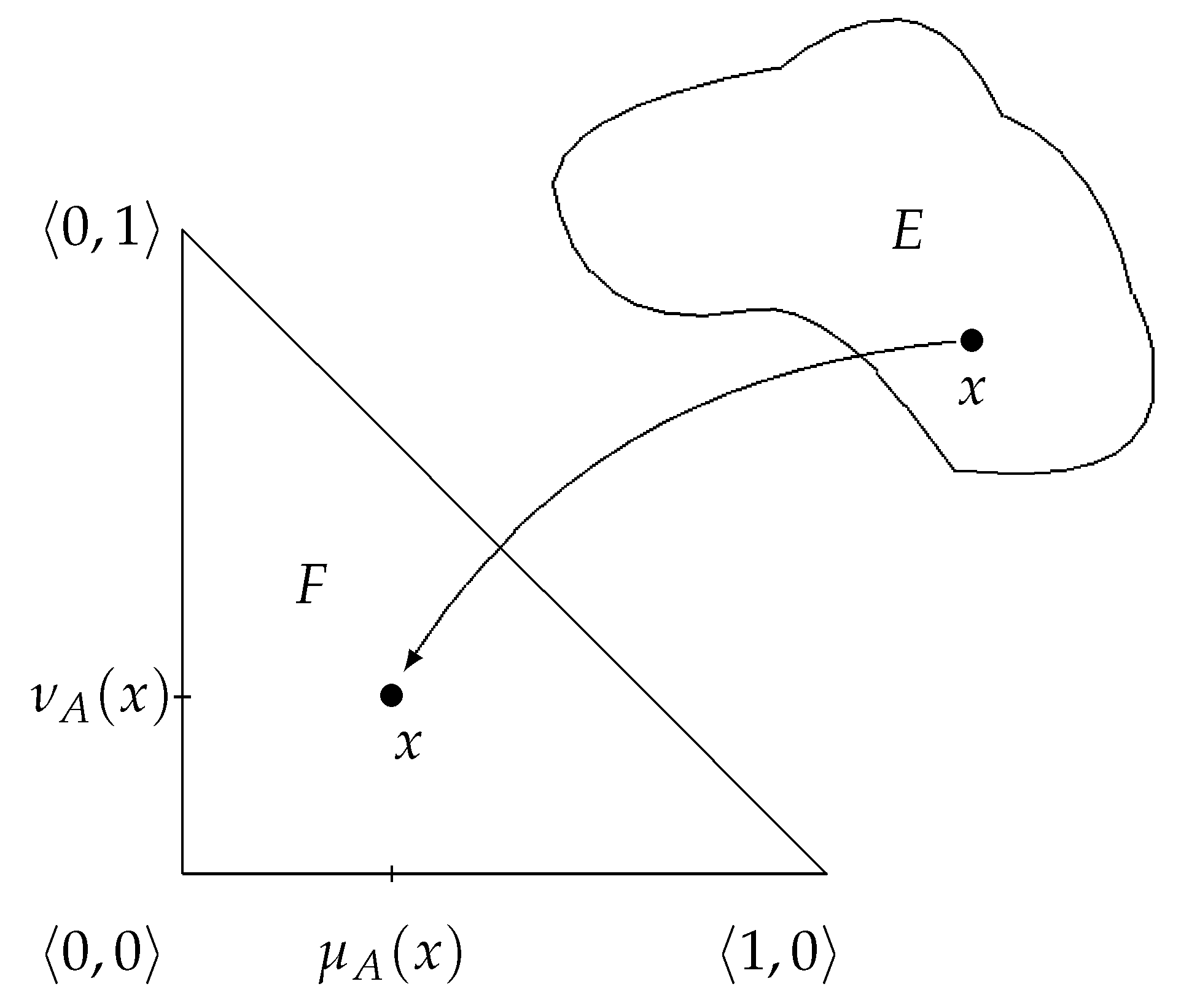
Having in mind the well-known interpretation of an intuitionistic fuzzy set onto a triangle F, as illustrated in Figure 1 (see [3,4]), we will show in a stepwise manner the way of constructing the geometrical interpretation of the element

$$〈x,\frac{{\mu }_A\left(x\right)+{\mu }_B\left(x\right)}{{\mu }_A\left(x\right)+{\nu }_A\left(x\right)+{\mu }_B\left(x\right)+{\nu }_B\left(x\right)},\frac{{\nu }_A\left(x\right)+{\nu }_B\left(x\right)}{{\mu }_A\left(x\right)+{\nu }_A\left(x\right)+{\mu }_B\left(x\right)+{\nu }_B\left(x\right)}〉,$$

when we have the geometrical interpretation of x about both IFSs A and B, i.e., $\langle x,{\mu }_A\left(x\right),{\nu }_A\left(x\right)\rangle$ and $\langle x,{\mu }_B\left(x\right),{\nu }_B\left(x\right)\rangle$. We will remind that the point with coordinates $\langle 1,0\rangle$ represents in the IFS triangle the complete $Truth$, and the point with coordinates $\langle 0,1\rangle$ represents the complete $Falsity$.

3.1. Algorithm for Construction of Operation ∆

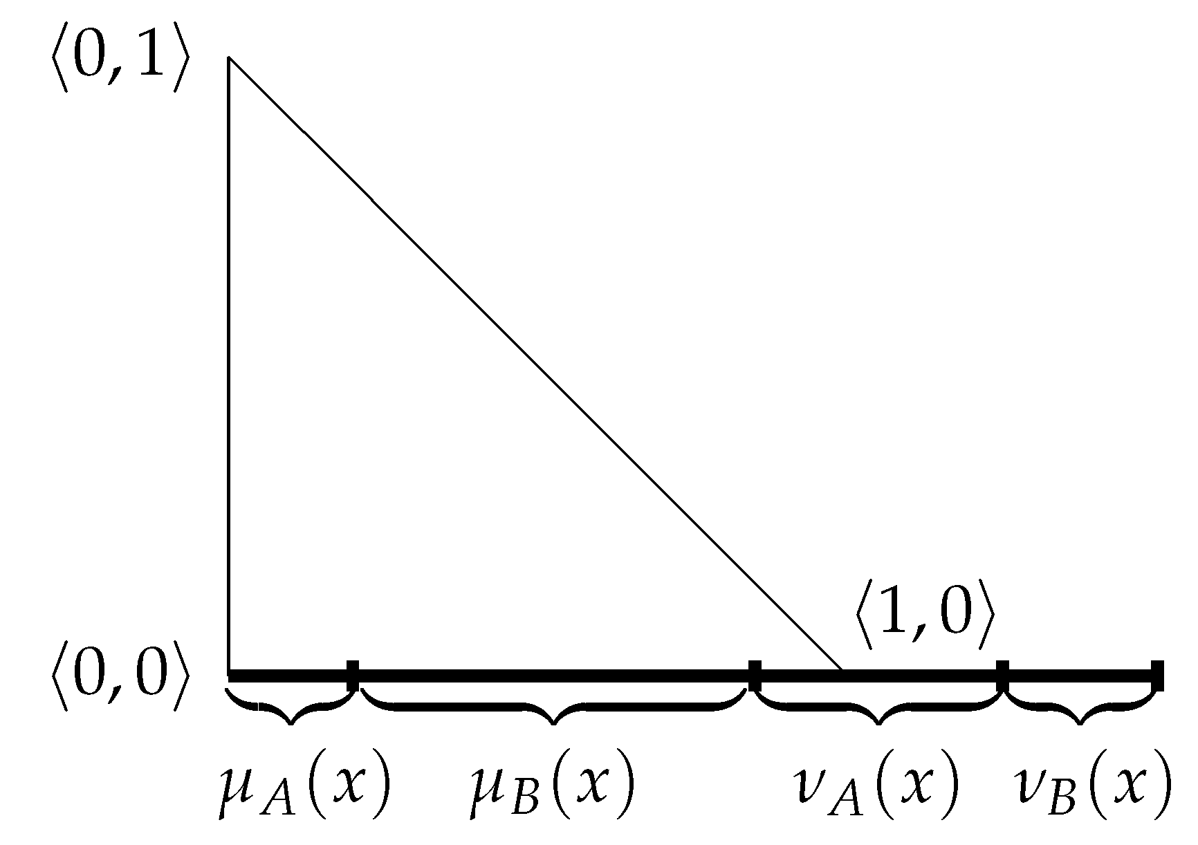
Step 1.

In Figure 2, we draw a section of length ${\mu }_A\left(x\right)+{\mu }_B\left(x\right)+{\nu }_A\left(x\right)+{\nu }_B\left(x\right)$ for the case when this length is a positive number.

Note: There are different cases for the length of this section as compared with the unitary length of the triangle’s side, but the procedure is similar in all the cases. In the special case, when the length is zero, obviously the result coincides with the point with coordinates $\langle 0,0\rangle$ which in the IFS theory is interpretation of the complete uncertainty.

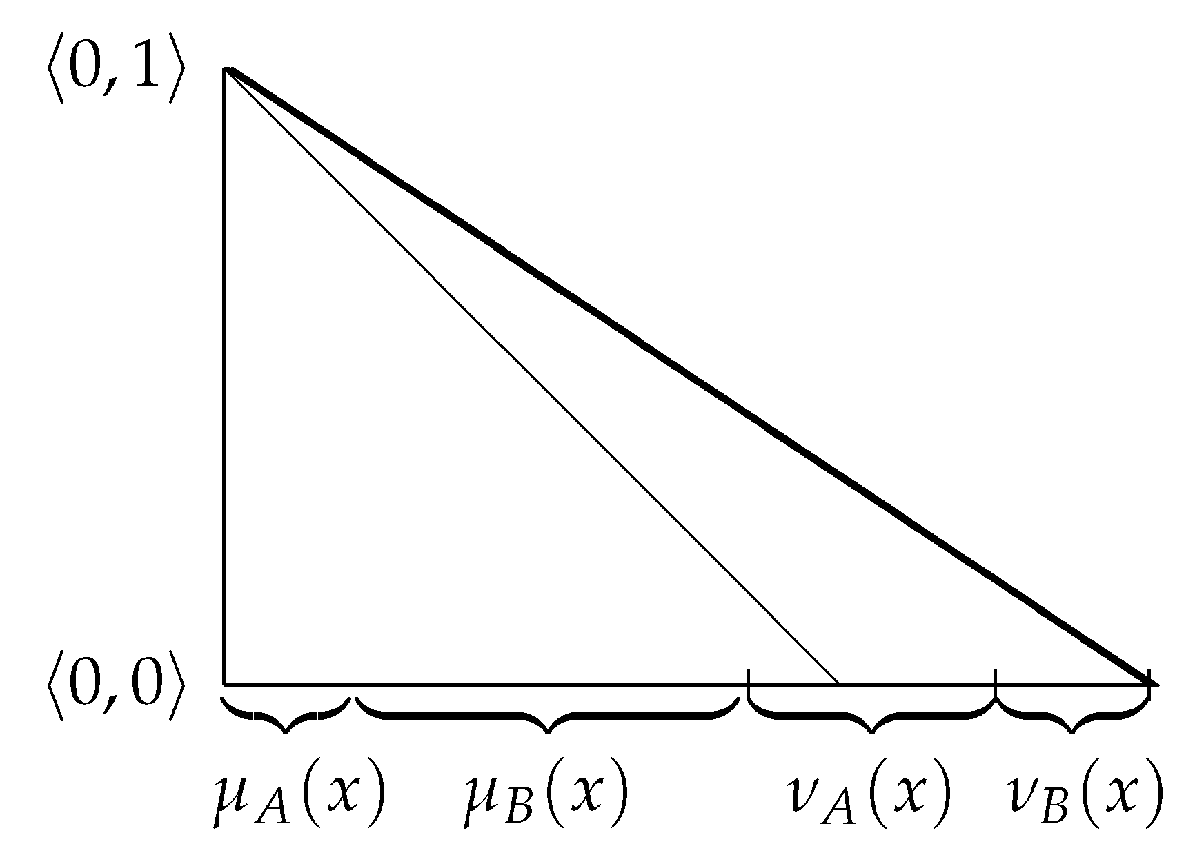
Step 2.

We connect the point with coordinates $\langle {\mu }_A\left(x\right)+{\mu }_B\left(x\right)+{\nu }_A\left(x\right)+{\nu }_B\left(x\right),0\rangle$ with the point with coordinates $\langle 0,1\rangle$ (see Figure 3), constructing a line.

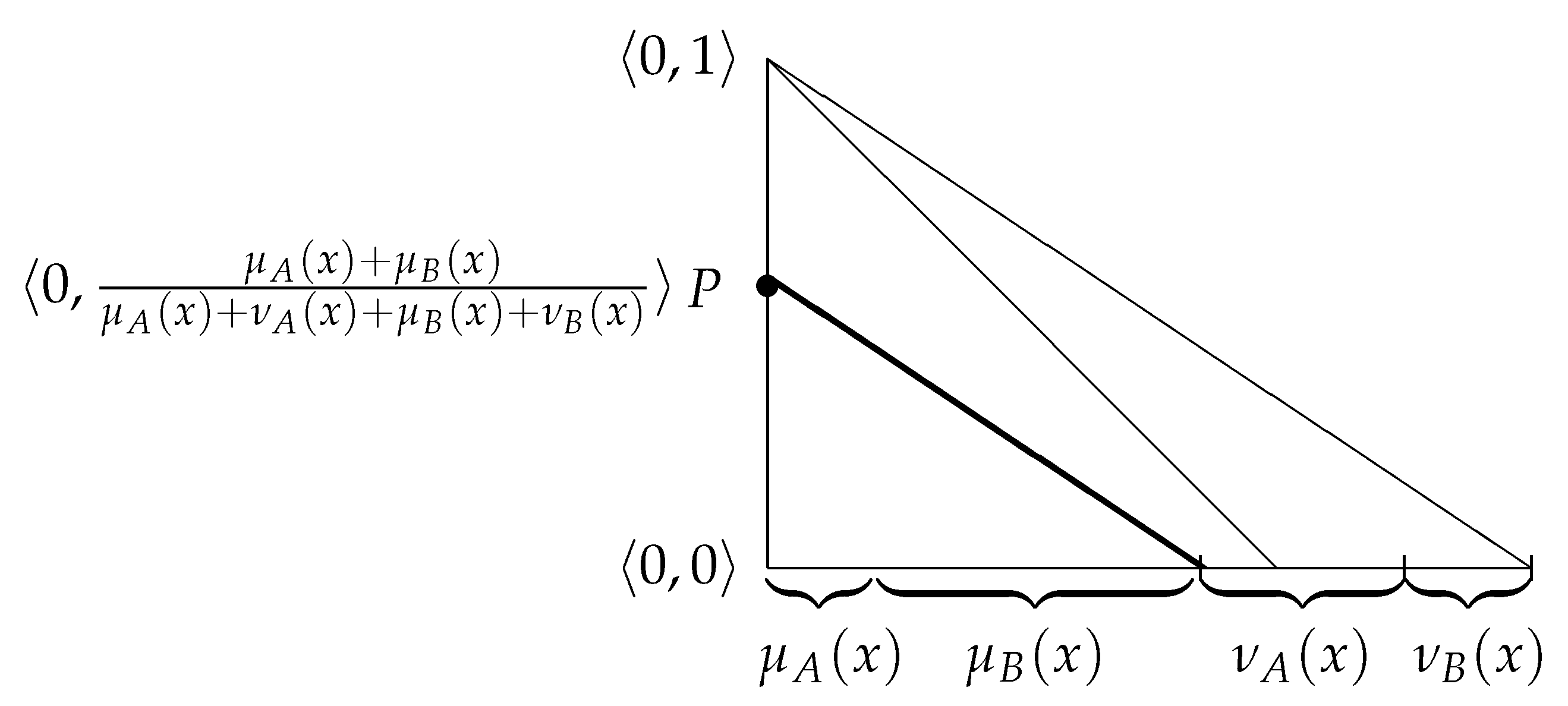
Step 3.

After this, we construct the line from point $\langle {\mu }_A\left(x\right)+{\mu }_B\left(x\right),0\rangle$ in such a way that is parallel to the previous one. It crosses the ordinate at point P. It is easily calculated that the coordinates of point P are $〈0,\frac{{\mu }_A\left(x\right)+{\mu }_B\left(x\right)}{{\mu }_A\left(x\right)+{\nu }_A\left(x\right)+{\mu }_B\left(x\right)+{\nu }_B\left(x\right)}〉$ (see Figure 4).

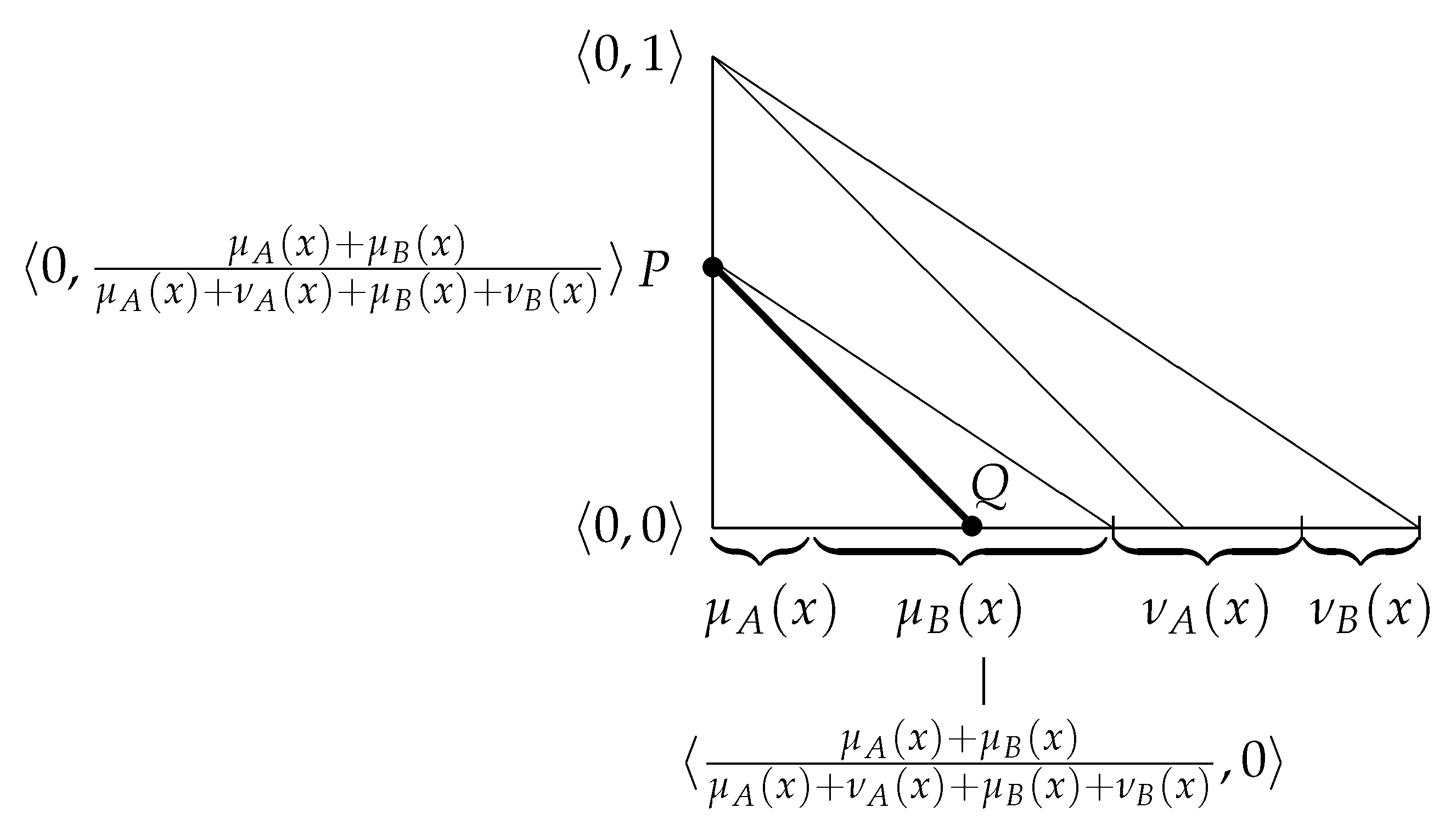
Step 4.

We construct a line from point P that is parallel to the hypotenuse of the IFS-interpretation triangle. The line crosses the abscissa at point Q (see Figure 5). Its coordinates are $〈\frac{{\mu }_A\left(x\right)+{\mu }_B\left(x\right)}{{\mu }_A\left(x\right)+{\nu }_A\left(x\right)+{\mu }_B\left(x\right)+{\nu }_B\left(x\right)},0〉$.

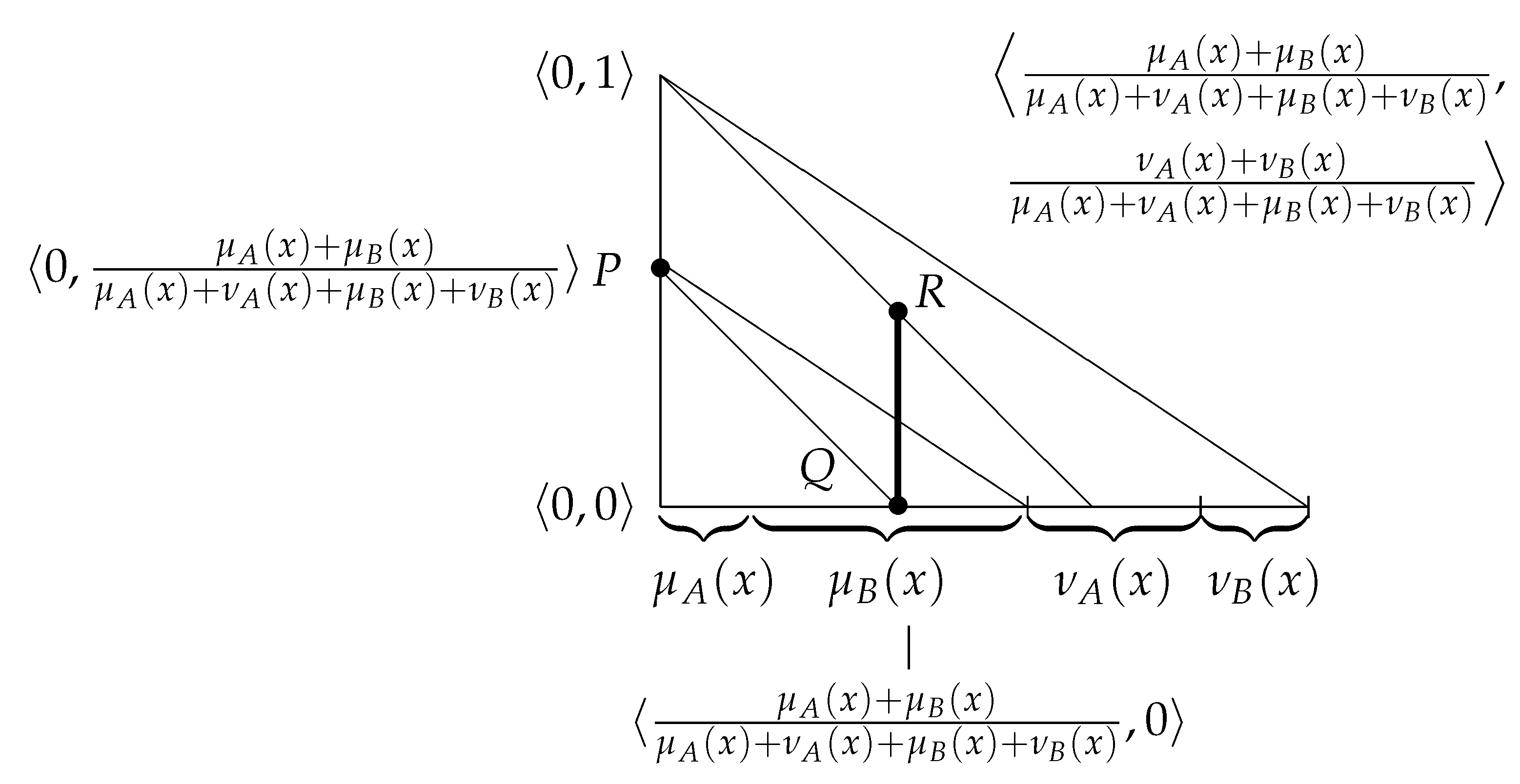
Step 5.

Finally, we construct a perpendicular from point Q to the hypotenuse of the IFS-interpretation triangle. The perpendicular crosses the hypotenuse in point R (see Figure 6). Its coordinates are $〈\frac{{\mu }_A\left(x\right)+{\mu }_B\left(x\right)}{{\mu }_A\left(x\right)+{\nu }_A\left(x\right)+{\mu }_B\left(x\right)+{\nu }_B\left(x\right)},\frac{{\nu }_A\left(x\right)+{\nu }_B\left(x\right)}{{\mu }_A\left(x\right)+{\nu }_A\left(x\right)+{\mu }_B\left(x\right)+{\nu }_B\left(x\right)}〉$.

Therefore, point R represents the geometrical interpretation of element x in the IFS $A∆B$.

The procedure is identical regardless of whether the sum ${\mu }_A\left(x\right)+{\mu }_B\left(x\right)+{\nu }_A\left(x\right)+{\nu }_B\left(x\right)$ is greater than or less then 1, the only difference is whether the constructions are within or outside of the triangle.

3.2. Properties of Operation ∆

It is directly seen that for every two IFSs A and B:

$$A∆B=B∆A,$$

i.e., the operation ∆ is commutative, but it is not associative.

The following statement, proven for the new operation ∆, gives an analogue of some sense to the De Morgan’s Laws.

Theorem 1.

For every two IFSs A and B:

$$\neg (\neg A∆\neg B)=A∆B.$$

Proof. 

Let the IFSs A and B be given. Then

$$\begin{array}{cc}\hfill \neg (\neg A∆\neg B)& =\neg (\left\{\langle x,{\nu }_A\left(x\right),{\mu }_A\left(x\right)\rangle \right|x\in E\}∆\left\{\langle x,{\nu }_B\left(x\right),{\mu }_B\left(x\right)\rangle \right|x\in E\})\hfill \\ \hfill & =\neg \left\{〈x,\frac{{\nu }_A\left(x\right)+{\nu }_B\left(x\right)}{{\mu }_A\left(x\right)+{\nu }_A\left(x\right)+{\mu }_B\left(x\right)+{\nu }_B\left(x\right)},\frac{{\mu }_A\left(x\right)+{\mu }_B\left(x\right)}{{\mu }_A\left(x\right)+{\nu }_A\left(x\right)+{\mu }_B\left(x\right)+{\nu }_B\left(x\right)}〉|x\in E\right\}\hfill \\ \hfill & =\left\{〈x,\frac{{\mu }_A\left(x\right)+{\mu }_B\left(x\right)}{{\mu }_A\left(x\right)+{\nu }_A\left(x\right)+{\mu }_B\left(x\right)+{\nu }_B\left(x\right)},\frac{{\nu }_A\left(x\right)+{\nu }_B\left(x\right)}{{\mu }_A\left(x\right)+{\nu }_A\left(x\right)+{\mu }_B\left(x\right)+{\nu }_B\left(x\right)}〉|x\in E\right\}\hfill \\ \hfill & =A∆B.\hfill \end{array}$$

This completes the proof. □

Let for the IFS A:

$$2A=A∆A$$

and for each natural number $n\ge 2$

$$nA=(n-1)A∆A.$$

Then the following theorem is valid, which gives an analogue of some sense to the Fixed Point Theorem.

Theorem 2.

For each IFS A and for each natural number $n\ge 2$

$$nA=\left\{〈x,\frac{{\mu }_A\left(x\right)}{{\mu }_A\left(x\right)+{\nu }_A\left(x\right)},\frac{{\nu }_A\left(x\right)}{{\mu }_A\left(x\right)+{\nu }_A\left(x\right)}〉|x\in E\right\}.$$

(2)

Proof. 

For the proof, we use the method of mathematical induction. Let $n=2$. Then

$$\begin{array}{cc}\hfill 2A& =A∆A\hfill \\ \hfill & =\left\{〈x,\frac{2{\mu }_A\left(x\right)}{2({\mu }_A\left(x\right)+{\nu }_A\left(x\right))},\frac{2{\nu }_A\left(x\right)}{2({\mu }_A\left(x\right)+{\nu }_A\left(x\right))}〉|x\in E\right\}\hfill \\ \hfill & =\left\{〈x,\frac{{\mu }_A\left(x\right)}{{\mu }_A\left(x\right)+{\nu }_A\left(x\right)},\frac{{\nu }_A\left(x\right)}{{\mu }_A\left(x\right)+{\nu }_A\left(x\right)}〉|x\in E\right\}.\hfill \end{array}$$

Let us assume that for some natural number $n\ge 2$ (2) is valid. Then

$$\begin{array}{cc}\hfill (n+1)A& =nA∆A\hfill \\ \hfill & =\left\{〈x,\frac{{\mu }_A\left(x\right)}{{\mu }_A\left(x\right)+{\nu }_A\left(x\right)},\frac{{\nu }_A\left(x\right)}{{\mu }_A\left(x\right)+{\nu }_A\left(x\right)}〉|x\in E\right\}∆A\hfill \\ \hfill & =\left\{〈x,\frac{\frac{{\mu }_A\left(x\right)}{{\mu }_A\left(x\right)+{\nu }_A\left(x\right)}+{\mu }_A\left(x\right)}{\frac{{\mu }_A\left(x\right)}{{\mu }_A\left(x\right)+{\nu }_A\left(x\right)}+\frac{{\nu }_A\left(x\right)}{{\mu }_A\left(x\right)+{\nu }_A\left(x\right)}+{\mu }_A\left(x\right)+{\nu }_A\left(x\right)},\right.\hfill \\ \hfill & \left.\frac{\frac{{\nu }_A\left(x\right)}{{\mu }_A\left(x\right)+{\nu }_A\left(x\right)}+{\nu }_A\left(x\right)}{\frac{{\mu }_A\left(x\right)}{{\mu }_A\left(x\right)+{\nu }_A\left(x\right)}+\frac{{\nu }_A\left(x\right)}{{\mu }_A\left(x\right)+{\nu }_A\left(x\right)}+{\mu }_A\left(x\right)+{\nu }_A\left(x\right)}〉|x\in E\right\}\hfill \\ \hfill & =\left\{〈x,\frac{\frac{{\mu }_A\left(x\right)}{{\mu }_A\left(x\right)+{\nu }_A\left(x\right)}(1+{\mu }_A\left(x\right)+{\nu }_A\left(x\right))}{1+{\mu }_A\left(x\right)+{\nu }_A\left(x\right)},\frac{\frac{{\nu }_A\left(x\right)}{{\mu }_A\left(x\right)+{\nu }_A\left(x\right)}(1+{\mu }_A\left(x\right)+{\nu }_A\left(x\right))}{1+{\mu }_A\left(x\right)+{\nu }_A\left(x\right)}〉|x\in E\right\}\hfill \\ \hfill & =\left\{〈x,\frac{{\mu }_A\left(x\right)}{{\mu }_A\left(x\right)+{\nu }_A\left(x\right)},\frac{{\nu }_A\left(x\right)}{{\mu }_A\left(x\right)+{\nu }_A\left(x\right)}〉|x\in E\right\}.\hfill \end{array}$$

This completes the proof. □

Corollary 1.

For each IFS A and for each natural number $n\ge 2$

$$nA=A∆U^{\ast }.$$

In [1,3], the two simplest intuitionistic fuzzy modal operators are defined by

$$\square A=\left\{\langle x,{\mu }_A\left(x\right),1-{\mu }_A\left(x\right)\rangle \right|x\in E\},$$

$$♢A=\left\{\langle x,1-{\nu }_A\left(x\right),{\nu }_A\left(x\right)\rangle \right|x\in E\}.$$

We can check directly that for every two IFSs A and B:

$$\square (A∆B)=A∆B,$$

$$♢(A∆B)=A∆B,$$

and, more generally, for each real number $\alpha \in [0,1]$:

$$D_{\alpha }(A∆B)=A∆B,$$

where the operator $D_{\alpha }$ is defined in [3] by

$$D_{\alpha }\left(A\right)=\left\{\langle x,{\mu }_A\left(x\right)+\alpha (1-{\mu }_A\left(x\right)-{\nu }_A\left(x\right)),{\nu }_A\left(x\right)+(1-\alpha )(1-{\mu }_A\left(x\right)-{\nu }_A\left(x\right))\rangle \right|x\in E\}.$$

The next two theorems give the connections between the operation ∆ on one hand and the classical modal operators over IFS Necessity and Possibility, on the other hand.

Theorem 3.

For every two IFSs A and B:

$$\square A∆\square B\subseteq \square (A∆B),$$

$$♢A∆♢B\supseteq ♢(A∆B).$$

Proof. 

Let the two IFSs A and B be given. Then

$$\begin{array}{cc}\hfill \square A∆\square B& =\left\{\langle x,{\mu }_A\left(x\right),1-{\mu }_A\left(x\right)\rangle \right|x\in E\}∆\left\{\langle x,{\mu }_B\left(x\right),1-{\mu }_B\left(x\right)\rangle \right|x\in E\}\hfill \\ \hfill & =\left\{〈x,\frac{{\mu }_A\left(x\right)+{\mu }_B\left(x\right)}{{\mu }_A\left(x\right)+1-{\mu }_A\left(x\right)+{\mu }_B\left(x\right)+1-{\mu }_B\left(x\right)},\right.\hfill \\ \hfill & \left.\frac{1-{\mu }_A\left(x\right)+1-{\mu }_B\left(x\right)}{{\mu }_A\left(x\right)+1-{\mu }_A\left(x\right)+{\mu }_B\left(x\right)+1-{\mu }_B\left(x\right)}〉|x\in E\right\}\hfill \\ \hfill & =\left\{〈x,\frac{{\mu }_A\left(x\right)+{\mu }_B\left(x\right)}{2},1-\frac{{\mu }_A\left(x\right)+{\mu }_B\left(x\right)}{2}〉|x\in E\right\}\hfill \\ \hfill & \subseteq \square \left\{〈x,\frac{{\mu }_A\left(x\right)+{\mu }_B\left(x\right)}{{\mu }_A\left(x\right)+{\nu }_A\left(x\right)+{\mu }_B\left(x\right)+{\nu }_B\left(x\right)},\frac{{\nu }_A\left(x\right)+{\nu }_B\left(x\right)}{{\mu }_A\left(x\right)+{\nu }_A\left(x\right)+{\mu }_B\left(x\right)+{\nu }_B\left(x\right)}〉|x\in E\right\}\hfill \\ \hfill & =\square (A∆B).\hfill \end{array}$$

The inclusion is valid because for every four numbers $a,b,c,d\in [0,1]$ such that $a+b+c+d>0$:

$$\frac{a+c}{a+b+c+d}\ge \frac{a+c}{2}$$

and hence

$$\frac{b+d}{a+b+c+d}\le 1-\frac{a+c}{2}.$$

The second inclusion is checked in the same manner. □

Theorem 4.

For every two IFSs A and B:

$$\square A\cap \square B\subseteq A∆B\subseteq ♢A\cup ♢B.$$

Proof. 

First, for every four numbers $a,b,c,d\in [0,1]$ so that $a+b\le 1,c+d\le 1$ we will prove the inequalities:

$$\min (a,c)\le \frac{a+c}{a+b+c+d}\le 1-\min (b,d).$$

Really, let $a\ge c$. Then

$$\frac{a+c}{a+b+c+d}-\min (a,c)=\frac{a+c}{a+b+c+d}-c\ge \frac{a+c}{2}-c\ge 0.$$

If $a<c$, then

$$\frac{a+c}{a+b+c+d}-\min (a,c)=\frac{a+c}{a+b+c+d}-a\ge \frac{a+c}{2}-a\ge 0.$$

Therefore,

$$\min (a,c)\le \frac{a+c}{a+b+c+d}.$$

Using this inequality, we obtain

$$\min (b,d)\le \frac{b+d}{a+b+c+d}=1-\frac{a+c}{a+b+c+d},$$

i.e.,

$$\frac{a+c}{a+b+c+d}\le 1-\min (b,d).$$

Now, using these inequalities, we check that

$$\square A\cap \square B=\left\{\langle x,{\mu }_A\left(x\right),1-{\mu }_A\left(x\right)\rangle \right|x\in E\}\cap \left\{\langle x,{\mu }_B\left(x\right),1-{\mu }_B\left(x\right)\rangle \right|x\in E\}$$

$$=\left\{\langle x,\min ({\mu }_A\left(x\right),{\mu }_B\left(x\right)),\max (1-{\mu }_A\left(x\right),1-{\mu }_B\left(x\right))\rangle \right|x\in E\}$$

$$=\left\{\langle x,\min ({\mu }_A\left(x\right),{\mu }_B\left(x\right)),1-\min ({\mu }_A\left(x\right),{\mu }_B\left(x\right))\rangle \right|x\in E\}$$

$$\subseteq \left\{〈x,\frac{{\mu }_A\left(x\right)+{\mu }_B\left(x\right)}{{\mu }_A\left(x\right)+{\nu }_A\left(x\right)+{\mu }_B\left(x\right)+{\nu }_B\left(x\right)},\frac{{\nu }_A\left(x\right)+{\nu }_B\left(x\right)}{{\mu }_A\left(x\right)+{\nu }_A\left(x\right)+{\mu }_B\left(x\right)+{\nu }_B\left(x\right)}〉|x\in E\right\}$$

$$\subseteq \left\{\langle x,1-\min ({\nu }_A\left(x\right),{\nu }_B\left(x\right)),\min ({\nu }_A\left(x\right),{\nu }_B\left(x\right))\rangle \right|x\in E\}$$

$$=\left\{\langle x,\max (1-{\nu }_A\left(x\right),1-{\nu }_B\left(x\right)),\min ({\nu }_A\left(x\right),{\nu }_B\left(x\right))\rangle \right|x\in E\}$$

$$=\left\{\langle x,1-{\nu }_A\left(x\right),{\nu }_A\left(x\right)\rangle \right|x\in E\}\cup \left\{\langle x,1-{\nu }_B\left(x\right),{\nu }_B\left(x\right)\rangle \right|x\in E\}$$

$$=♢A\cup ♢B.$$

This completes the proof. □

Following the idea from [5], where operation ∆ was extended from binary to n-ary form for n IFPs, here we extend operation ∆ from binary to n-ary form for n IFSs $A_1,A_2,\dots ,A_n$ as follows:

$$∆(A_1,A_2,\dots ,A_n)=\left\{〈x,\frac{{\displaystyle \sum _{i=1}^n}{\mu }_{A_i}\left(x\right)}{{\displaystyle \sum _{i=1}^n}({\mu }_{A_i}\left(x\right)+{\nu }_{A_i}\left(x\right))},\frac{{\displaystyle \sum _{i=1}^n}{\nu }_{A_i}\left(x\right)}{{\displaystyle \sum _{i=1}^n}({\mu }_{A_i}\left(x\right)+{\nu }_{A_i}\left(x\right))}〉|x\in E\right\}.$$

Therefore, when E is a finite set, we can define the operator

$${\displaystyle ◬}A=\left\{〈x,\frac{{\displaystyle \sum _{x\in E}}{\mu }_A\left(x\right)}{{\displaystyle \sum _{x\in E}}({\mu }_A\left(x\right)+{\nu }_A\left(x\right))},\frac{{\displaystyle \sum _{x\in E}}{\nu }_A\left(x\right)}{{\displaystyle \sum _{x\in E}}({\mu }_A\left(x\right)+{\nu }_A\left(x\right))}〉|x\in E\right\}.$$

Hence,

$${\displaystyle ◬◬}A={\displaystyle ◬}A.$$

Therefore, the operation ∆ and the operator ◬ can be used for the procedure for de-i-fuzzification, as it is discussed in the next section.

4. Discussion and Conclusions

The new operation ∆ defined over IFSs and studied in the present paper can be used for aggregation of some experts’ evaluations, when the result should contain no degree of uncertainty.

The considerations regarding the transformation of IFSs to FSs (de-i-fuzzification) or real numbers (crisipification) have been a matter of research since 1995 in the works of Angelov [8], Ansari et al. [9], Ban et al. [6], Atanassova and Sotirov [10], Anzilli and Facchinetti [11]. For instance, in [6], the authors use as the base of the de-i-fuzzification the operator $D_{\alpha }$ (for the definition see [3,6]) and determine the minimal distance, in Hamming and in Euclidean sense, between the IFS A and the FS $D_{\alpha }\left(A\right)$.

Let us have an expert’s evaluation in the form of an ordered pair $\langle a,b\rangle$, where $a+b>1$. Since it represents an element outside of the intuitionistic fuzzy triangle, it is an incorrect IFP in terms of the definition of IFS. For this case, a simple modification of the operation ∆, when applied over incorrect IFPs $\langle a,b\rangle$, can be also used for the procedure for rectification of the unconscientious experts’ evaluations, as described in [4,14].

Really, for every unconscientious evaluation $\langle a,b\rangle$, where $a,b\in [0,1],a+b>1$, the rectification of this incorrect evaluation is given by

$$\langle a,b\rangle ∆\langle a,b\rangle =\langle a,b\rangle ∆\langle 0,0\rangle =〈\frac{a}{a+b},\frac{b}{a+b}〉.$$

For example, if an expert has given an unconscientious evaluation $\langle 0.3,0.9\rangle$, then as a result of the operation ∆ we obtain the rectified value $\langle 0.25,0.75\rangle$, which already is a correct IFP.

On a side note, a similar procedure can be used according to the SNCF distance (called, also, French metro metric, radial metric, or other), which appears in the mathematical literature on distances (see, e.g., [15]). In this case, for any point $\langle a,b\rangle$ the closest one is the point $\langle a^{\prime },b^{\prime }\rangle$ satisfying the condition

$$\langle a^{\prime },b^{\prime }\rangle =〈\frac{a}{a+b},\frac{b}{a+b}〉,$$

therefore, the ∆ operation is a de-i-fuzzification operation. The properties of this kind of de-i-fuzzification, as well as new properties of operation ∆ and operator ◬ will be studied in next legs of authors’ research.

References

- Atanassov, K. Intuitionistic fuzzy sets. Int. J. Bioautom. 2016, 20, S1–S6. [Google Scholar]
- Zadeh, L. Fuzzy sets. Inf. Control 1965, 8, 338–353. [Google Scholar] [CrossRef] [Green Version]
- Atanassov, K. Intuitionistic Fuzzy Sets: Theory and Applications; Springer: Berlin/Heidelberg, Germany, 1999. [Google Scholar]
- Atanassov, K. On Intuitionistic Fuzzy Sets Theory; Springer: Berlin/Heidelberg, Germany, 2012. [Google Scholar]
- Atanassova, L. A new operator over intitionistic fuzzy sets. Notes Intuit. Fuzzy Sets 2020, 26, 23–27. [Google Scholar]
- Ban, A.; Kacprzyk, J.; Atanassov, K. On de-i-fuzzification of intuitionistic fuzzy sets. Comptes Rendus L’Academie Bulg. Des Sci. 2008, 61, 1535–1540. [Google Scholar]
- van Leekwijck, W.; Kerre, E.E. Defuzzification: Criteria and classification. Fuzzy Sets Syst. 1999, 108, 159–178. [Google Scholar] [CrossRef]
- Angelov, P. Crispification: Defuzzification of Intuitionistic Fuzzy Sets. BUSEFAL 1995, 64, 51–55. [Google Scholar]
- Ansari, A.Q.; Siddiqui, S.A.; Alvi, J.A. Mathematical Techniques To Convert Intuitionistic Fuzzy Sets Into Fuzzy Sets. Notes Intuit. Fuzzy Sets 2004, 10, 13–17. [Google Scholar]
- Atanassova, V.; Sotirov, S. A new formula for de-i-fuzzification of intuitionistic fuzzy sets. Notes Intuit. Fuzzy Sets 2012, 18, 49–51. [Google Scholar]
- Anzilli, L.; Facchinetti, G. A New Proposal of Defuzzification of Intuitionistic Fuzzy Quantities. In Novel Developments in Uncertainty Representation and Processing; Series “Advances in Intelligent Systems and Computing”; Atanassov, K., Ed.; Springer: Cham, Switzerland, 2016; pp. 185–195. [Google Scholar]
- Buhaescu, T. On the convexity of intuitionistic fuzzy sets. In Itinerant Seminar on Functional Equations, Approximation and Convexity; “Babeş-Bolyai” University Faculty of Mathematics and Physics Research Seminars: Cluj-Napoca, Romania, 1988; pp. 137–144. [Google Scholar]
- Atanassov, K.; Szmidt, E.; Kacprzyk, J. On intuitionistic fuzzy pairs. Notes Intuit. Fuzzy Sets 2013, 19, 1–13. [Google Scholar]
- Dworniczak, P. A distance based correction of the unconscientious experts’ evaluations. Notes Intuit. Fuzzy Sets 2015, 21, 5–17. [Google Scholar]
- Deza, E.; Deza, M.M. Encyclopedia of Distances; Springer: Berlin/Heidelberg, Germany, 2009. [Google Scholar]
Figure 1.
Geometrical interpretation of an element into the intuitionistic fuzzy interpretational triangle.
Figure 2.
First step.
Figure 3.
Second step.
Figure 4.
Third step.
Figure 5.
Fourth step.
Figure 6.
Fifth step.
Publisher’s Note: MDPI stays neutral with regard to jurisdictional claims in published maps and institutional affiliations. |
© 2021 by the authors. Licensee MDPI, Basel, Switzerland. This article is an open access article distributed under the terms and conditions of the Creative Commons Attribution (CC BY) license (https://creativecommons.org/licenses/by/4.0/).
Share and Cite
MDPI and ACS Style
Atanassova, L.; Dworniczak, P. On the Operation ∆ over Intuitionistic Fuzzy Sets. Mathematics 2021, 9, 1518. https://doi.org/10.3390/math9131518
AMA Style
Atanassova L, Dworniczak P. On the Operation ∆ over Intuitionistic Fuzzy Sets. Mathematics. 2021; 9(13):1518. https://doi.org/10.3390/math9131518
Chicago/Turabian StyleAtanassova, Lilija, and Piotr Dworniczak. 2021. "On the Operation ∆ over Intuitionistic Fuzzy Sets" Mathematics 9, no. 13: 1518. https://doi.org/10.3390/math9131518
Note that from the first issue of 2016, this journal uses article numbers instead of page numbers. See further details here.