A Review of Matrix SIR Arino Epidemic Models

Abstract

Many of the models used nowadays in mathematical epidemiology, in particular in COVID-19 research, belong to a certain subclass of compartmental models whose classes may be divided into three “$(x,y,z)$” groups, which we will call respectively “susceptible/entrance, diseased, and output” (in the classic SIR case, there is only one class of each type). Roughly, the ODE dynamics of these models contains only linear terms, with the exception of products between x and y terms. It has long been noticed that the reproduction number $\mathcal{R}$ has a very simple Formula in terms of the matrices which define the model, and an explicit first integral Formula is also available. These results can be traced back at least to Arino, Brauer, van den Driessche, Watmough, and Wu (2007) and to Feng (2007), respectively, and may be viewed as the “basic laws of SIR-type epidemics”. However, many papers continue to reprove them in particular instances. This motivated us to redraw attention to these basic laws and provide a self-contained reference of related formulas for $(x,y,z)$ models. For the case of one susceptible class, we propose to use the name SIR-PH, due to a simple probabilistic interpretation as SIR models where the exponential infection time has been replaced by a PH-type distribution. Note that to each SIR-PH model, one may associate a scalar quantity $Y(t)$ which satisfies “classic SIR relations”,which may be useful to obtain approximate control policies.

1. Introduction

Motivation. Mathematical epidemiology may be said to have started with the SIR ODE model, which saw its birth in the works of Kermack–McKendrick [1]. This was initially applied to model the Bombay plague of 1905–06, and later to measles [2], smallpox, chickenpox, mumps, typhoid fever and diphtheria, and recently to the COVID-19 pandemic—see, for example in [3,4,5,6,7,8,9,10,11,12,13,14,15,16,17,18], to cite just a few representatives of a huge literature.

Note that during the COVID-19 pandemic, researchers have relied mostly on models with quadratic interactions (linear force of infection), which belong furthermore to a particular class [19,20,21,22] of “$(x,y,z)$” models. Here, x denotes “entrance/susceptible” classes; y denotes diseased classes, which must converge asymptotically to 0; and z denotes output classes. These models are very useful; to make references to them easier, we propose to call them matrix-SIR (SYR) models, and also SIR-PH [21], when $x\in {\mathbb{R}}^1$.

Contents. We begin by recalling in Section 2 several basic explicit formulas for the SIR model. Section 3 presents the corresponding SIR-PH generalizations, and Section 4 offers some applications: the SEIHRD model [23,24,25,26,27], which adds to the classic SEIR (susceptible + exposed + infectious + recovered) a hospitalized (H) class and a dead class (D); the SEICHRD model [28] which adds a critically ill class (C); the SEIARD [29] and SEIAHR/SEIRAH(D) models [30,31,32,33,34,35,36], which add an asymptomatic class (A); and the S$I^3$QR model [37]. This is just a sample chosen from some of our favorite COVID papers. We note in passing that they seem though all unaware of the existence of the Arino and Feng Formulas (12) and (17).

Finally, Section 5 reviews briefly the case of several classes of susceptibles. This topic requires further development; we include it however due to the recognized importance of heterogeneity factors.

2. The Classic Kermack–McKendrick SIR Epidemic Model

The SIR process $(S(t),I(t),R(t),t\ge 0)$ divides a population of size N undergoing an epidemic into three classes called “susceptibles, infectives, and removed”. One may also work with the corresponding fractions $\mathsf{s}(t)=\frac{S(t)}{N},\mathsf{i}(t)=\frac{I(t)}{N},$ and $\mathsf{r}(t)=1-\mathsf{s}(t)-\mathsf{i}(t)$. It is assumed that only susceptible individuals can get infected. After having been infectious for some time, an individual recovers and may not become susceptible again. “Viewed from far away”, this yields the SIR model with demography [1,38]

$$\begin{array}{cc}\hfill S^{\prime }(t)& =-\frac{\beta }{N}S(t)I(t)+\xi \left(N-S(t)\right),\hfill \\ \hfill I^{\prime }(t)& =I(t)\left(\frac{\beta }{N}S(t)-\gamma -\xi \right),\hfill \\ \hfill R^{\prime }(t)& =\gamma I(t)-\xi R(t),\hfill \end{array}$$

(1)

where

• N is the total, constant population size.
• $R^{\prime }(t)$, the number of removed per unit time, is the only quantity which is clearly observable, at least in the easy case when the removed are dead, as was the case of the original study of the Bombay plague [1].
• $\xi$ is the population death rate, assumed to equal the birth rate.
• $\gamma$ is the removal rate of the infectious, which equals 1/duration of the infection (under the stochastic model of exponential infection durations, this is the reciprocal of the expected duration).
• $\beta$, the infection rate, models the probability that a contact takes place between an infected and a susceptible, and that it results in infection.

Note that

• The sum $S+I+R=N$ is conserved and each value is positive, so the values of $S,I,R$ remain in the interval $[0,N]$.
• This system has a unique solution, as (given the boundedness of $S,I$, and R), the RHS above is Lipschitz.

From now on, we will assume that $\xi =0$, and work with the fractions $\mathsf{s},\mathsf{i},\mathsf{r}$, which satisfy

$$\begin{array}{cc}\hfill {\mathsf{s}}^{\prime }(t)& =-\beta \mathsf{s}(t)\mathsf{i}(t),\hfill \\ \hfill {\mathsf{i}}^{\prime }(t)& =\mathsf{i}(t)[\beta \mathsf{s}(t)-\gamma ],\hfill \\ \hfill {\mathsf{r}}^{\prime }(t)& =\gamma \mathsf{i}(t).\hfill \end{array}$$

(2)

We will call this the classic SIR model, see Figure 1. Note that

• $\mathsf{s}(t)$ is monotonically decreasing and $\mathsf{r}(t)$ is monotonically increasing, to, say, $s_{\infty },r_{\infty }$; therefore convergence to some fixed stable point $(s_{\infty },i_{\infty },r_{\infty })$ must hold.
• the equilibrium set of stable points is $(s,0,1-s),s\in [0,1].$
• solutions starting in the domain

  $$\mathcal{D}:=\left\{(s,i,r):s>0,i>0,r\ge 0,s+i+r\le 1\right\}$$

  cannot leave it.
• The second equation of (1) implies the so-called threshold phenomenon: if

  $$\mathcal{R}:=\frac{\beta }{\gamma }\le 1$$

  (3)

  then $\mathsf{i}(t)$ decreases always, without any intervention. $\mathcal{R}$ is called reproduction number, and it models the number of susceptibles infected by one infectious (expected number, under more sophisticated stochastic, branching models). A convenient analytical definition, as the Perron–Frobenius eigenvalue of the “next-generation matrix” [39,40,41], is available as well.
  To avoid trivialities, we will assume $\mathcal{R}>1$ from now on.
• When $\mathcal{R}>1$, the epidemic grows iff $\mathsf{s}>1/\mathcal{R}$, i.e., until the susceptibles $\mathsf{s}(t)$ reach the immunity threshold

  $$\mathsf{\Theta }:=\frac{1}{\mathcal{R}}=\frac{\gamma }{\beta },$$

  (4)

  after which infections decline.

An advantage of the classic SIR model is that it is essentially solvable explicitly:

• We can eliminate $\mathsf{r}$ from the system using the invariant $\mathsf{s}+\mathsf{i}+\mathsf{r}=1$.
• It can easily be verified that

  $$\mu (s,i):=s+i-\frac{1}{\mathcal{R}}ln(s)$$

  (5)

  is invariant, (note that we have used different fonts for (s,i,r) when they are functions of t, and standard fonts when they are not), so that i is explicitly given by

  $$i_{\mathcal{R}}(s)=-s+\frac{1}{\mathcal{R}}ln(s)+{\mu }_{\mathcal{R}}(s_0,i_0),$$

  (6)

  and the full system (2) can be reduced to the single ODE

  $${\mathsf{s}}^{\prime }(t)=-\beta \mathsf{s}(s_0+i_0-\mathsf{s})-\gamma \mathsf{s}ln\left(\frac{\mathsf{s}}{s_0}\right).$$

  (7)
• The maximal value of the infected $\mathsf{i}$, achieved when $\mathsf{s}=1/\mathcal{R}$, is

  $$i_{max}=i_{max,\mathcal{R}}(s_0,i_0)=i_0+s_0-\frac{1+ln(s_0\mathcal{R})}{\mathcal{R}}=i_0+\frac{H(s_0\mathcal{R})}{\mathcal{R}},H(\mathcal{R})=\mathcal{R}-1-ln(\mathcal{R}).$$

  (8)
• By differentiating the right-hand side of (7), one finds that the maximal value of the “newly infected” $-{\mathsf{s}}^{\prime }=\beta \mathsf{i}\mathsf{s}$ is achieved when

  $$\mathsf{s}=\mathsf{i}+\frac{\gamma }{\beta },\mathsf{s}=-\frac{1}{2\mathcal{R}}{L}_{-1}\left[-2\mathcal{R}{s}_0{e}^{-1-\mathcal{R}(s_0+i_0)}\right],$$

  (9)

  where the Lambert function $L_{-1}$ is a real inverse of $L(z)=z{e}^z$– see for example [42,43,44]. Bounding $\mathsf{s}\mathsf{i}$ is one interesting possibility for accomodating ICU constraints [45] (2.20).
• The infectious class converges to 0 and the susceptible and recovered converge monotonically to limits which may be expressed in terms of the “Lambert–W(right)” function $L_0$.

Let us note that accurate numerical solutions of the evolution of the SIR or other compartmental epidemic may be obtained very quickly.

3. SIR-PH Epidemics with One Susceptible Class (SIR Epidemics with Phase-Type “Disease Time”)

It has been known for a long while that $\mathcal{R}$ and the final size for many compartmental model epidemics may be explicitly expressed in terms of the matrices which define the model, and the works in [19,20,46,47] offer a quite general framework of “xyz” models which ensures this. We believe that these formulas have not received the attention they deserve (they keep being reproved), and decided therefore to review them below; we will call them matrix- SIR models.

A particular but revealing case is that when there is only one susceptible class, which we will call SIR-PH, following Riano [21], who emphasized its probabilistic interpretation—see also in [48].

Definition 1.

A “SIR-PH $(\overrightarrow{\alpha },V,\mathit{\beta },W)$ epidemic" contains a homogeneous susceptible class, but vector “diseased" state $\overrightarrow{\mathsf{i}}$ (which may contain latent/exposed, infective, asymptomatic, etc.) and vector removed states (healthy, dead, vaccinated, etc.). It is defined by an ODE system:

$$\begin{array}{c}\hfill \left\{\begin{array}{cc}& {\mathsf{s}}^{\prime }(t)=-\mathsf{s}(t)\overrightarrow{\mathsf{i}}(t)\mathit{\beta }\hfill \\ & \overrightarrow{\mathsf{i}}{}^{\prime }(t)=\mathsf{s}(t)\overrightarrow{\mathsf{i}}(t)\mathit{\beta }\overrightarrow{\alpha }+\overrightarrow{\mathsf{i}}(t)A\hfill \\ & {\overrightarrow{\mathsf{r}}}^{\prime }(t)=\overrightarrow{\mathsf{i}}(t)W\hfill \end{array}\right.\end{array}$$

(10)

where

1.

$\overrightarrow{\mathsf{i}}(t)\in {\mathbb{R}}^n$ is a row vector whose components are fractions of diseased individuals of various types, which must satisfy $\overrightarrow{\mathsf{i}}(\infty )=0$.

2.

$\mathit{\beta }\in {\mathbb{R}}^n$ is a column vector whose components represent the relative transmission ability of the various disease classes.

3.

$\overrightarrow{\alpha }\in {\mathbb{R}}^n$ is a probability row vector with the components representing the fractions of susceptibles entering into the corresponding disease compartments, when infection occurs.

4.

A is a $n\times n$ Markovian sub-generator matrix describing rates of transition between the diseased classes $\overrightarrow{\mathsf{i}}$ (i.e., a Markovian generator matrix for which the sum of at least one row is strictly negative). Alternatively, $V:=-A$ is a non-singular M-matrix ( M-matrix is a real matrix V with $v_{ij}\le 0,\forall i\ne j,$ and having eigenvalues whose real parts are nonnegative [49]).

5.

$\overrightarrow{\mathsf{r}}(t)\in {\mathbb{R}}^p$ is a row vector which must satisfy $\overrightarrow{\mathsf{r}}(\infty )>0,$ whose components represent (fractions of) various classes which survive at the end of an infection.

6.

W is a $n\times p$, matrix whose components represent the rates at which classes of diseased individuals become recovered. We assume that the $n\times (n+p)$ matrix $\tilde{V}=\left(\begin{array}{cc}A& W\end{array}\right)$ has row sums 0 (which implies that the total population $N(t)=\mathsf{s}(t)+\overrightarrow{\mathsf{i}}(t)\mathbf{1}+\overrightarrow{\mathsf{r}}(t)\mathbf{1}$ is constant).

We turn now to a deceivingly simple particular example of the SIR-PH model, which explains its name.

Remark 1.

Probabilistic interpretation of SIR-PH epidemics.For simplicity, let us group all the output classes of (10) into one $\mathsf{r}=\overrightarrow{\mathsf{r}}\mathbf{1}$, where 1 is a column vector of ones of appropriate dimension (here p), yielding

$$\left\{\begin{array}{c}{\mathsf{s}}^{\prime }(t)=-\mathsf{s}(t)\overrightarrow{\mathsf{i}}(t)\mathit{\beta }\hfill \\ {\overrightarrow{\mathsf{i}}}^{\prime }(t)=\mathsf{s}(t)\overrightarrow{\mathsf{i}}(t)\mathit{\beta }\overrightarrow{\alpha }+\overrightarrow{\mathsf{i}}(t)A\hfill \\ {\mathsf{r}}^{\prime }(t)=\overrightarrow{\mathsf{i}}(t)\mathit{a}\mathbf{,}\hfill \end{array}\right.$$

(11)

where we put $\mathit{a}:=W1=(-A)\mathbf{1}$.

(11) emphasizes the fact that SIR-PH models are in one to one correspondence with laws of phase-type $(\overrightarrow{\alpha },A)$ [21] (21).

Let us recall now, as known essentially since the work in [50]—see also [51] (Theorem 2.2.7)—that under proper scaling, the expected fractions $\mathsf{s}(t)$, $\mathsf{i}(t),\mathsf{r}(t)$ of stochastic SIR (One such model stipulates that each infective $j=1,\cdots ,J$ infects a randomly chosen susceptible, at encounter times which belong to independent Poisson processes $P^j(t),j=1,\cdots ,J$, of rate β, and that infection durations are i.i.d. r.v.’s which areexponentially distributedat the end of which the individual recovers (or dies).) and more general compartmental models obey a “law of large numbers/fluid limit" which recovers the deterministic epidemic.

As an example, the SIR-PH model (10) may be derived as limit of a stochastic SIR model in which the exponential infection time has been replaced by a phase-type $(\overrightarrow{\alpha },A)$ “dwell period” [48].

Proposition 1.

For processes defined by (10), with $V=-A$ a non-singular M-matrix, the basic reproduction number is given by [19] (Theorem 2.1) (This can be also derived as the expected number of susceptibles infected during a dwell period, for the stochastic model (the so-called “survival method”)—see the work in [52] for an excellent review).

$$\mathcal{R}=\overrightarrow{\alpha }{V}^{-1}\mathit{\beta }.$$

(12)

A disease-free equilibrium $(s_0,\overrightarrow{0},{\overrightarrow{r}}_0)$ is asymptotically stable iff $s_0<\frac{1}{\mathcal{R}}.$

To illustrate the power of the SIR-PH formalism, consider now the case with two diseased states—latent and infectious—with phase-type dwell times, parametrized by $({\overrightarrow{\alpha }}_e,A_e)$ and $({\overrightarrow{\alpha }}_i,A_i)$, respectively. Using the well-known convolution formula—see, for example, [53] (Theorem 3.1.26) we find that formulas like (12) (see other examples of such formulas below) still apply, with $(\overrightarrow{\alpha },A,\mathit{\beta })$ given by

$$\overrightarrow{\alpha }=({\overrightarrow{\alpha }}_e,0),A=\left(\begin{array}{cc}{A}_e& {\mathit{a}}_e{\overrightarrow{\alpha }}_i\\ 0& A_i\end{array}\right),\mathit{\beta }=\left(\begin{array}{c}0\\ 0\\ ⋮\\ {\beta }_{i,1}\\ {\beta }_{i,2}\\ ⋮\end{array}\right).$$

(13)

The “epidemic dwell strucure” $(\overrightarrow{\alpha },A,\mathit{\beta })$ of examples with more complicated network structures for the diseased may be constructed using Kronecker sums of the matrices defining each component.

Let us give now an example which does not in general belong to the SIR-PH class.

Example 1.

The SIRV model—see, for example, in [54]—is defined by

$$\begin{array}{cc}\hfill {\mathsf{s}}^{\prime }(t)& =-\mathsf{s}(t)\left(\beta \mathsf{i}(t)+{\gamma }_s\right),\hfill \\ \hfill {\mathsf{i}}^{\prime }(t)& =\mathsf{i}(t)\left[\beta \mathsf{s}(t)-{\gamma }_i\right],\hfill \\ \hfill {\mathsf{r}}^{\prime }(t)& ={\gamma }_i\mathsf{i}(t),\hfill \\ \hfill {\mathsf{v}}^{\prime }(t)& ={\gamma }_s\mathsf{s}(t).\hfill \end{array}$$

(14)

This is of the form (10) with $\overrightarrow{\mathsf{i}}=(\mathsf{i}),\overrightarrow{\mathsf{r}}=(\mathsf{r},\mathsf{v})$ iff ${\gamma }_s=0$.

In the opposite case ${\gamma }_s\ne 0$, one may still compute an invariant (Note that ${\gamma }_s>0$ has been used for modeling vaccination, and ${\gamma }_s<0$ has been used for modeling loss of immunity)

$$\mu (s,i):=\beta (s+i)-\gamma ln(s)+\mathsf{v}ln(i),$$

(15)

and for fixed s, putting $\tilde{\gamma }=\frac{\gamma }{{\gamma }_s},\tilde{\beta }=\frac{\beta }{{\gamma }_s},{\tilde{\mu }}_0=\frac{{\mu }_0}{{\gamma }_s}$, it holds that i is explicitly given by

$$i(s)=\frac{1}{\tilde{\beta }}{L}_0\left[\tilde{\beta }{s}^{\tilde{\gamma }}{e}^{{\tilde{\mu }}_0-\tilde{\beta }s}\right].$$

(16)

When ${\gamma }_s>0$, the final size is $s_{\infty }=0$.

We provide now a list of several formulas, obtained by replacing $\mathsf{i}$ in SIR by a scalar linear combination (17) [47]. They are all easily proved; however the formula for the maximal value of the newly infected involves also a second linear combination $\mathsf{y}$ (21).

Proposition 2.

For processes defined by (10), with $V=-A$ a non-singular M-matrix, it holds that:

1.

The following weighted sum of the diseased variables [47] (24)

$$Y(t)=\frac{\overrightarrow{\mathsf{i}}(t)V^{-1}\mathit{\beta }}{\overrightarrow{\alpha }{V}^{-1}\mathit{\beta }}=\frac{1}{\mathcal{R}}\overrightarrow{\mathsf{i}}(t)V^{-1}\mathit{\beta }$$

(17)

has the property that

$$\frac{dY}{d\mathsf{s}}=\frac{\frac{1}{\mathcal{R}}\overrightarrow{\mathsf{i}}(t)\left(\mathsf{s}(t)\mathit{\beta }\overrightarrow{\alpha }-V\right)V^{-1}\mathit{\beta }}{-\mathsf{s}(t)\overrightarrow{\mathsf{i}}(t)\mathit{\beta }}=\frac{\overrightarrow{\mathsf{i}}(t)\mathit{\beta }\left(\mathsf{s}(t)\mathcal{R}-1\right)}{-\mathcal{R}\mathsf{s}(t)\overrightarrow{\mathsf{i}}(t)\mathit{\beta }}=-1+\frac{1}{\mathcal{R}\mathsf{s}},$$

(18)

and that

$$\left\{\begin{array}{c}z(t)=\mu (\mathsf{s}(t),Y(t)):=Y(t)+\mathsf{s}(t)-\frac{1}{\mathcal{R}}ln[\mathsf{s}(t)],\hfill \\ Z(t)=e^{-\mathcal{R}z(t)}=\mathsf{s}(t)e^{-\mathcal{R}(\mathsf{s}(t)+Y(t))}\hfill \end{array}\right.$$

(19)

are constant along the paths of the dynamical system (10) .

The solution of $Z(s)=Z(0)$ with respect to $\mathsf{s}$ may be expressed in terms of

$$\mathsf{s}(t)=-\frac{1}{\mathcal{R}}{L}_0\left[-\mathcal{R}{Z}_0{e}^{\mathcal{R}Y(t)}\right],$$

(20)

where $[-e^{-1},\infty )\ni z\to L_0(z)\in [-1,\infty )$ is the principal branch of the Lambert-W function.

2.

The derivative with respect to time is

$$\frac{dY}{dt}=\left(\mathsf{s}-\frac{1}{\mathcal{R}}\right)\overrightarrow{\mathsf{i}}\mathit{\beta }:=\left(\mathsf{s}-\frac{1}{\mathcal{R}}\right)\mathsf{y}.$$

(21)

Therefore, $\frac{dY}{dt}=0=\frac{dY}{ds}$ iff $s={\mathcal{R}}^{-1}$.

3.

The maximum value of Y occurs for $s=min[1/\mathcal{R},1]$. In the case $\mathcal{R}>1$, this yields [47] (Section 2.1):

$$Y_0+{\mathsf{s}}_0-Y^{\ast }-\frac{1}{\mathcal{R}}=\frac{1}{\mathcal{R}}ln({\mathsf{s}}_0\mathcal{R}),$$

(22)

by the conservation of $Y(t)+\mathsf{s}(t)-\frac{1}{\mathcal{R}}ln(\mathsf{s}(t))$ between the time 0 and the time $t_{1/\mathcal{R}}$ of reaching the immunity threshold).

4.

The final size of the susceptibles satisfies [19] (Theorem 5.1):

$$ln[{\mathsf{s}}_0/{\mathsf{s}}_{\infty }]=\mathcal{R}\left({\mathsf{s}}_0-{\mathsf{s}}_{\infty }\right)+\overrightarrow{\mathsf{i}}{}_0{V}^{-1}\mathit{\beta }=\mathcal{R}\left({\mathsf{s}}_0-{\mathsf{s}}_{\infty }+Y_0\right),$$

(23)

by the conservation of $Y(t)+\mathsf{s}(t)-\frac{1}{\mathcal{R}}ln(\mathsf{s}(t))$ between the times 0 and ∞; explicitly,

$${\mathsf{s}}_{\infty }=-\frac{1}{\mathcal{R}}{L}_0\left[-\mathcal{R}{Z}_0\right]=-\frac{1}{\mathcal{R}}{L}_0\left[-\mathcal{R}{s}_0{e}^{-\mathcal{R}(s_0+Y_0)}\right]$$

(24)

5.

The integrated infectives ${\overrightarrow{I}}^{(a,b)}={\int }_a^b\overrightarrow{\mathsf{i}}(s)ds$ satisfies

$$\left\{\begin{array}{c}{\overrightarrow{I}}^{(a,b)}V={\overrightarrow{J}}_a-{\overrightarrow{J}}_b,{\overrightarrow{J}}_s:=\overrightarrow{\mathsf{i}}(s)+s\overrightarrow{\alpha }\hfill \\ \left({\overrightarrow{J}}_a-{\overrightarrow{J}}_b\right)V^{-1}\mathit{\beta }=log(\frac{\mathsf{s}(a)}{\mathsf{s}(b)})\hfill \end{array}\right.,$$

(25)

and the total integrated infectives ${\overrightarrow{I}}^{(\infty )}={\int }_0^{\infty }\overrightarrow{\mathsf{i}}(s)ds$ satisfies [19] (6)

$${\overrightarrow{I}}^{(\infty )}V=\overrightarrow{\mathsf{i}}{}_0+(s_0-s_{\infty })\overrightarrow{\alpha }.$$

(26)

6.

The final size of the removed satisfies:

$${\overrightarrow{\mathsf{r}}}_{\infty }-{\overrightarrow{r}}_0=I^{(\infty )}W=\left(\overrightarrow{\mathsf{i}}{}_0+(s_0-s_{\infty })\overrightarrow{\alpha }\right)V^{-1}W,$$

(27)

7.

The value of the infected combination Y when $\mathsf{s}=1/\mathcal{R}$ is

$$Y_{max}=i_{max,\mathcal{R}}(s_0,\overrightarrow{\mathsf{i}}{}_0)=Y_0+s_0-\frac{1+ln(s_0\mathcal{R})}{\mathcal{R}}=i_0+\mathcal{R},H(\mathcal{R})=\mathcal{R}-1-ln(\mathcal{R}).$$

(28)

8.

The maximum size of the newly infected is achieved when

$$s(t)=\frac{{\mathsf{y}}^2+\mathcal{R}Y(t)}{\overrightarrow{\alpha }\mathit{\beta }\mathsf{y}}.$$

(29)

Remark 2.

In particular, for the SIR model (2),

$$log\left(\frac{\mathsf{s}(a)}{\mathsf{s}(b)}\right)=\beta I^{(a,b)}=\mathcal{R}(J_a-J_b),J=\mathsf{s}+\mathsf{i}.$$

(30)

Note that this has been used to model the total cost of an epidemic [55].

Remark 3.

Let us note that for control problems involving optimization objectives which only depend on $Y(t)$, we are effectively optimizing a SIR model; this SIR approximation may be used to offer practical solutions for optimizing more complicated compartmental models.

Example 2.

For SEIR, putting $\overrightarrow{\mathsf{i}}=(\mathsf{e},\mathsf{i})$, we may write

$$\begin{array}{c}\hfill \left\{\begin{array}{c}{\mathsf{s}}^{\prime }=-\beta \mathsf{s}\mathsf{i}\hfill \\ \overrightarrow{\mathsf{i}}{}^{\prime }=(\beta \mathsf{s}\mathsf{i}-{\gamma }_e\mathsf{e},{\gamma }_e\mathsf{e}-\gamma \mathsf{i})=\beta \mathsf{s}\mathsf{i}(1,0)-(\mathsf{e},\mathsf{i})\left(\begin{array}{cc}{\gamma }_e& -{\gamma }_e\\ 0& \gamma \end{array}\right)\hfill \\ {\mathsf{r}}^{\prime }=\gamma \mathsf{i}\hfill \end{array}\right.\end{array}$$

$$\mathit{so} \mathit{that}\left\{\begin{array}{c}\overrightarrow{\alpha }=(1,0)\hfill \\ \mathit{b}=\left(\begin{array}{c}0\\ \beta \end{array}\right)\hfill \\ V=\left(\begin{array}{cc}{\gamma }_e& -{\gamma }_e\\ 0& \gamma \end{array}\right)⟹V^{-1}=\frac{1}{\gamma {\gamma }_e}\left(\begin{array}{cc}\gamma & {\gamma }_e\\ 0& {\gamma }_e\end{array}\right),Y=\frac{\left(\begin{array}{c}\mathsf{e},\mathsf{i}\end{array}\right)\left(\begin{array}{cc}\gamma & {\gamma }_e\\ 0& {\gamma }_e\end{array}\right)\left(\begin{array}{c}0\\ \beta \end{array}\right)}{\left(\begin{array}{c}1,0\end{array}\right)\left(\begin{array}{cc}\gamma & {\gamma }_e\\ 0& {\gamma }_e\end{array}\right)\left(\begin{array}{c}0\\ \beta \end{array}\right)}=\mathsf{e}+\mathsf{i}\hfill \\ W=\left(\begin{array}{cc}0& \gamma \end{array}\right)\hfill \end{array}\right..$$

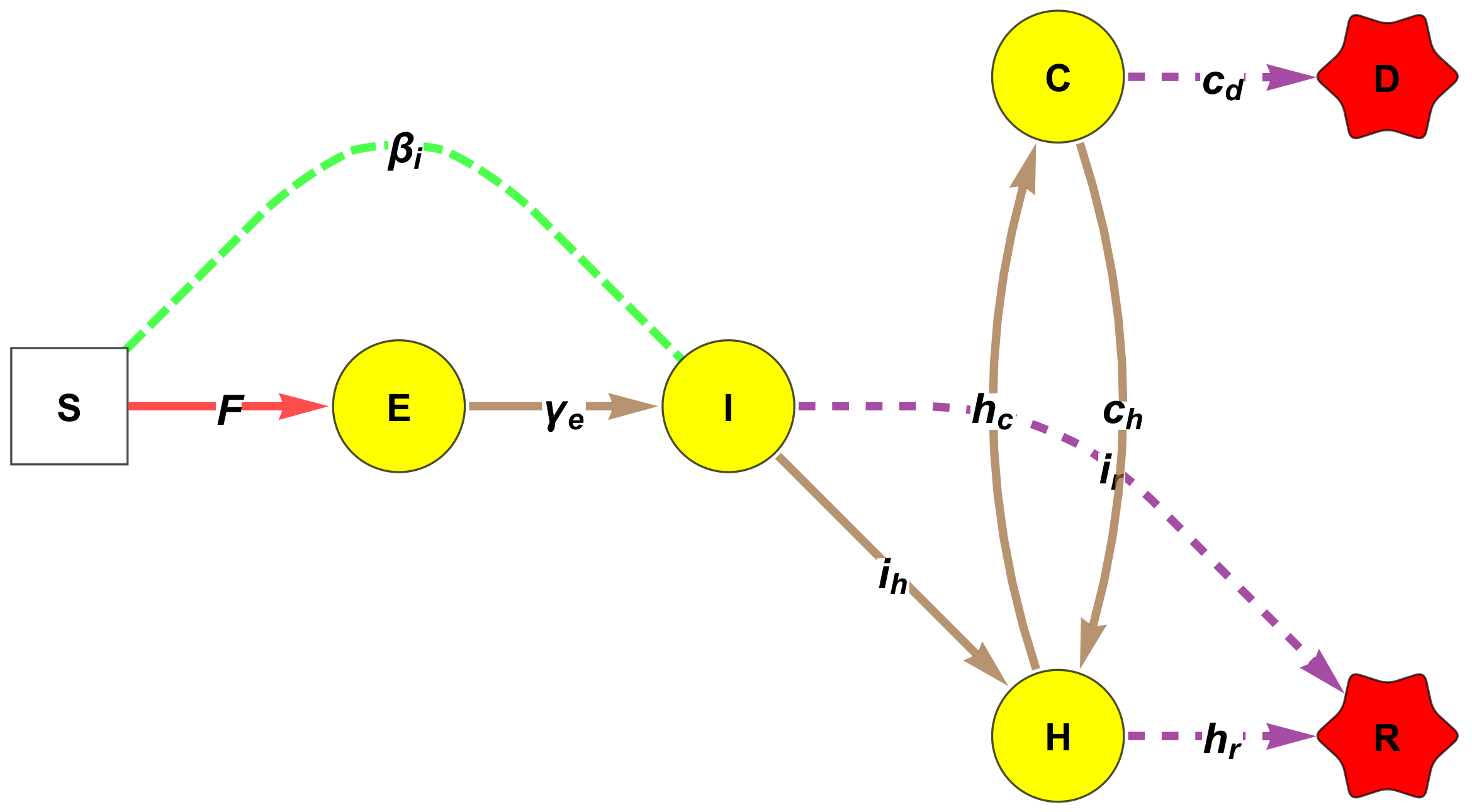
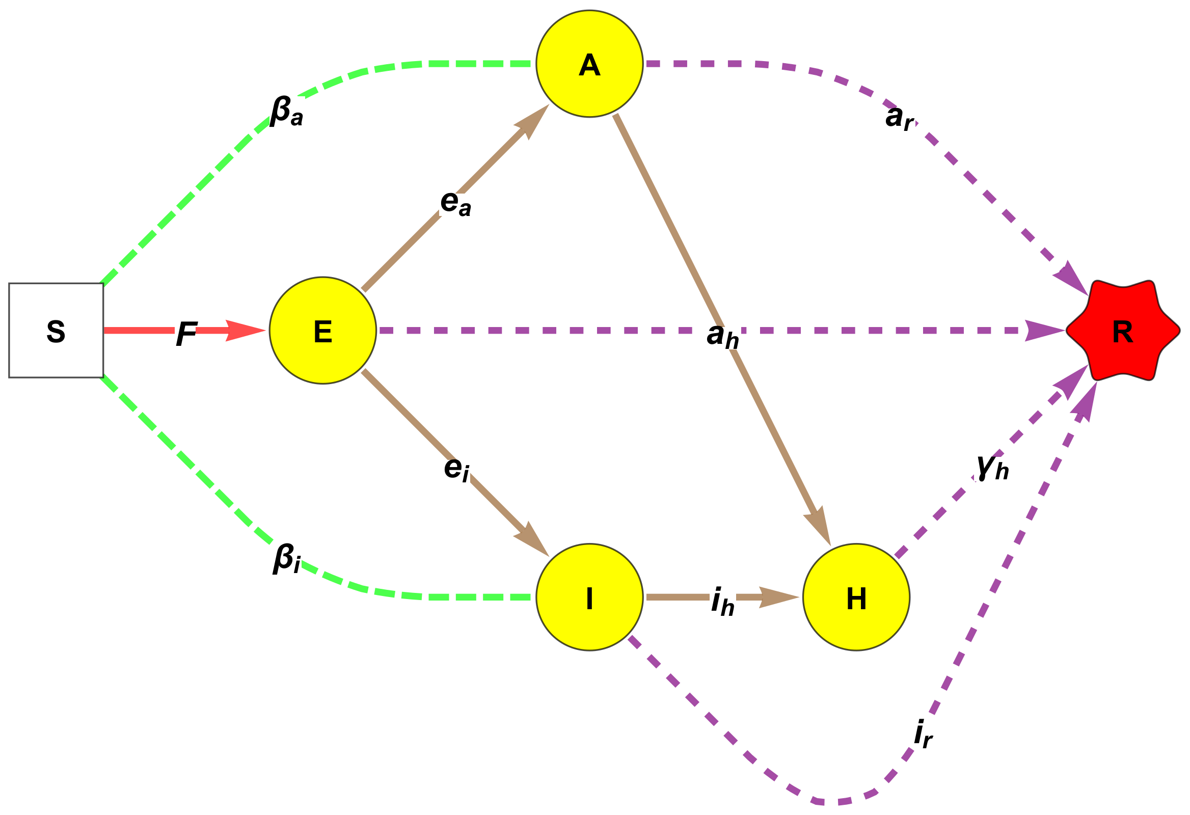
4. Examples of SIR-PH Models Used in COVID-19 Modelling

We derive now $\mathcal{R}$ and Y from (12), (17), for some popular compartmental models. Note that we will be reformulating the original results (which, unfortunately, have already appeared several times with different notations), using a unifying notation.

Example 3.

The SEIHRD model [23,24,25,26,27] has disease states $\overrightarrow{\mathsf{i}}=(\mathsf{e},\mathsf{i},\mathsf{h})$. We use here the version in [25] (we would rather call this S$I^2$HRD model) defined by,

$$\overrightarrow{\alpha }=\left(\begin{array}{c}1,0,0\end{array}\right),\mathit{\beta }=\left(\begin{array}{c}{\beta }_e\\ {\beta }_i\\ 0\end{array}\right),V=\left(\begin{array}{ccc}{\gamma }_e& -e_i& 0\\ 0& {\gamma }_i& -i_h\\ 0& 0& {\gamma }_h\end{array}\right),W=\left(\begin{array}{cc}{e}_r& 0\\ i_r& 0\\ h_r& h_d\end{array}\right),$$

where we denoted by ${\gamma }_e,{\gamma }_i,{\gamma }_h$ the sum of the constant rates out of $\mathsf{e},\mathsf{i},\mathsf{h},$ and by $i_h$ the rate out of $\mathsf{i}$ and reaching $\mathsf{h}$, etc. See Figure 2.

Then, $\mathcal{R}=\frac{{\beta }_e}{{\gamma }_e}+\frac{e_i}{{\gamma }_e}\frac{{\beta }_i}{{\gamma }_i}$ [25] (2), and $Y=\mathsf{e}+\mathsf{i}\frac{{\gamma }_e{\beta }_i}{{\beta }_e{\gamma }_i+e_i{\beta }_i}.$ When ${\beta }_e=0=e_r⟹\frac{e_i}{{\gamma }_e}=1$, we recover $\mathcal{R}=\frac{{\beta }_i}{{\gamma }_i}$ [24] and $Y=\mathsf{e}+\mathsf{i}.$

Example 4.

The SEIHCRD model of the work in [28], has disease states $\overrightarrow{\mathsf{i}}=(\mathsf{e},\mathsf{i},\mathsf{c})$ and is defined by

$$\mathit{\beta }=\left(\begin{array}{c}0\\ {\beta }_i\\ 0\\ 0\end{array}\right),\overrightarrow{\alpha }=\left(\begin{array}{c}1,0,0,0\end{array}\right),V=\left(\begin{array}{cccc}{\gamma }_e& -e_i& 0& 0\\ 0& {\gamma }_i& -i_h& 0\\ 0& 0& {\gamma }_h& -h_c\\ 0& 0& -c_h& {\gamma }_c\end{array}\right),W=\left(\begin{array}{cc}0& 0\\ i_r& 0\\ h_r& 0\\ 0& c_d\end{array}\right),$$

see Figure 3.

Then,

$$\mathcal{R}=\frac{{\beta }_i}{{\gamma }_i},Y=\mathsf{e}+\mathsf{i}.$$

Example 5.

The SEIRAH(SEIAHR) model [30,36] has disease states $\overrightarrow{\mathsf{i}}=(\mathsf{e},\mathsf{i},\mathsf{a},\mathsf{h})$ and is defined by

$$\mathit{\beta }=\left(\begin{array}{c}0\\ {\beta }_i\\ {\beta }_a\\ 0\end{array}\right),\overrightarrow{\alpha }=\left(\begin{array}{c}1,0,0,0\end{array}\right),V=\left(\begin{array}{cccc}{\gamma }_e& -e_i& -e_a& 0\\ 0& {\gamma }_i& 0& -i_h\\ 0& 0& {\gamma }_a& -a_h\\ 0& 0& 0& {\gamma }_h\end{array}\right),W=\left(\begin{array}{c}{e}_r\\ i_r\\ a_r\\ {\gamma }_h\end{array}\right).$$

See Figure 4 below.

Then,

$$\mathcal{R}=\frac{e_a}{{\gamma }_e}{\mathcal{R}}_a+\frac{e_i}{{\gamma }_e}{\mathcal{R}}_i,{\mathcal{R}}_i=\frac{{\beta }_i}{{\gamma }_i},{\mathcal{R}}_a=\frac{{\beta }_a}{{\gamma }_a},$$

and

$$Y=\mathsf{e}+\mathsf{i}\frac{{\mathcal{R}}_i}{\mathcal{R}}+\mathsf{a}\frac{{\mathcal{R}}_a}{\mathcal{R}}.$$

Example 6.

The S$I^{aps}$QR model (with asymptomatic, pre-symptomatic, and symptomatic infectious) [37,56] (3.2). See Figure 5;

The disease states are $\overrightarrow{\mathsf{i}}=({\mathsf{i}}_a,{\mathsf{i}}_p,{\mathsf{i}}_s,\mathsf{q})$, and the model is defined by

$$\mathit{\beta }=\left(\begin{array}{c}{\beta }_a\\ {\beta }_p\\ {\beta }_s\\ 0\end{array}\right),\overrightarrow{\alpha }=\left(\begin{array}{c}\varphi ,1-\varphi ,0,0\end{array}\right),V=\left(\begin{array}{cccc}{\gamma }_a& 0& 0& 0\\ 0& {\gamma }_p& -{\gamma }_p& 0\\ 0& 0& {\gamma }_s& -i_q\\ 0& 0& 0& \gamma {}_q\end{array}\right),W=\left(\begin{array}{c}{\gamma }_a\\ 0\\ i_{sr}\\ {\gamma }_q\end{array}\right).$$

Then, from the work in [37],

$$\mathcal{R}=\varphi \frac{{\beta }_a}{{\gamma }_a}+(1-\varphi )\left(\frac{{\beta }_p}{{\gamma }_p}+\frac{{\beta }_s}{{\gamma }_s}\right),$$

and,

$$Y=\frac{1}{\mathcal{R}}\left[{\mathsf{i}}_a{\mathcal{R}}_a+{\mathsf{i}}_p({\mathcal{R}}_p+{\mathcal{R}}_s)+{\mathsf{i}}_s{\mathcal{R}}_s\right],$$

where ${\mathcal{R}}_a:=\frac{{\beta }_a}{{\gamma }_a},{\mathcal{R}}_p:=\frac{{\beta }_p}{{\gamma }_p},and{\mathcal{R}}_s:=\frac{{\beta }_s}{{\gamma }_s}.$

5. ${\mathit{S}}^{(\mathit{m})}\mathit{YR}$ Models with $\mathit{m}$ Groups of Susceptibles

The SIR-compartment model makes the unrealistic assumption that the population through which the disease is spreading is well-mixed. However, differences in susceptibility and rates of contact between individuals strongly affect their likelihood of catching COVID-19. A model which attempts to capture this aspect is:

$$\begin{array}{c}\hfill \left\{\begin{array}{cc}& {\mathsf{s}}_k^{\prime }(t)=-{\mathsf{s}}_k(t)\overrightarrow{\mathsf{i}}(t){\mathit{\beta }}_k,k=1,\cdots ,m\hfill \\ & \overrightarrow{\mathsf{i}}{}^{\prime }(t)={\sum }_{k=1}^m{\mathsf{s}}_k(t)\overrightarrow{\mathsf{i}}(t){\mathit{\beta }}_k\overrightarrow{\alpha }-\overrightarrow{\mathsf{i}}(t)V\hfill \\ & {\overrightarrow{\mathsf{r}}}^{\prime }(t)=\overrightarrow{\mathsf{i}}(t)W\hfill \end{array}\right.\end{array}$$

(31)

Lemma 1.

A disease free equilibrium $(s_1,s_2,\cdots ,s_m,\overrightarrow{0},{\overrightarrow{r}}_0)$ of (31) is asymptotically stable iff $s\mathcal{R}<1,$ where $s={\sum }_k{s}_k$ and

$$\mathcal{R}=\sum _k\frac{s_k}{s}\overrightarrow{\alpha }{V}^{-1}{\mathit{\beta }}_k=\sum _k\frac{s_k}{s}{\mathcal{R}}_k,{\mathcal{R}}_k:=\overrightarrow{\alpha }{V}^{-1}{\mathit{\beta }}_k$$

(32)

is the spectral radius of the next generation matrix.

While the final size may also be obtained under this model [20] (Theorem 2.1), for transient behavior it is convenient to turn to a simpler model.

A Generalization of Heterogeneous SEIR

Assume now that ${\mathit{\beta }}_k={\beta }_k\mathit{\beta },$ where ${\beta }_k\in {\mathbb{R}}_{+}$ and W = $\mathit{\beta }\overrightarrow{w}$, where $\overrightarrow{w}$ is a row vector. Putting $\mathsf{y}=\overrightarrow{\mathsf{i}}\mathit{\beta }$, the system (31) becomes (Such dynamics was first considered in [57]).

$$\frac{dlog{\mathsf{s}}_k}{dt}=-{\beta }_k\mathsf{y},\frac{d\overrightarrow{\mathsf{i}}}{dt}=\left(\sum _{k=1}^m{\beta }_k{\mathsf{s}}_k\right)\mathsf{y}\overrightarrow{\alpha }-\overrightarrow{\mathsf{i}}V,\frac{d\overrightarrow{\mathsf{r}}}{dt}=\overrightarrow{\mathsf{i}}W=\mathsf{y}\overrightarrow{w},$$

(33)

and

$$\overrightarrow{\mathsf{r}}(t)={\int }_0^t\mathsf{y}(u)du\overrightarrow{w}:=I(t)\overrightarrow{w}.$$

(34)

It is convenient to reparametrize the model taking I as parameter, or, equivalently, by taking

$$\mathsf{r}=\overrightarrow{\mathsf{r}}\mathbf{1}=\gamma I,\gamma :=\overrightarrow{w}\mathbf{1}.$$

(35)

Solving

$$\frac{d}{dt}\left(log{\mathsf{s}}_k\right)=-{\beta }_k\mathsf{y}=-\frac{{\beta }_k}{\gamma }\frac{d}{dt}\mathsf{r},$$

we find that the system has a family of first integrals which includes

$$\left\{\begin{array}{c}\frac{1}{{\mathcal{R}}_1}log(s_1/s_1(0))=\cdots =\frac{1}{{\mathcal{R}}_k}log(s_k/s_k(0))=\cdots =\frac{1}{{\mathcal{R}}_m}log(s_m/s_m(0))=r(0)-r,\hfill \\ {\sum }_{k=1}^m{s}_k+{\sum }_{k=1}^n{y}_k+{\sum }_{k=1}^p{r}_k=1\hfill \end{array}\right..$$

(36)

Also

$${\mathsf{s}}_k(t)={\mathsf{s}}_k(0)e^{-{\beta }_{k}I(t)}={\mathsf{s}}_k(0)e^{-\frac{{\beta }_k}{\gamma }\mathsf{r}(t)},$$

(37)

where $\gamma$ is defined in (35).

We conclude with some preliminary results on this model.

Lemma 2.

(a) The authors of [58] put $\mathsf{s}(t)={\sum }_k{\mathsf{s}}_k(t),p_k={\mathsf{s}}_k(0)/\mathsf{s}(0)$. The solution of (33) satisfies the time-dependent SYR system:

$$\frac{d\mathsf{s}}{dt}=-a(t)\mathsf{s}(t)\mathsf{y}(t),\frac{d\overrightarrow{\mathsf{i}}}{dt}=\left(\sum _k{\beta }_k{\mathsf{s}}_k(t)\right)\mathsf{y}(t)\overrightarrow{\alpha }-\overrightarrow{\mathsf{i}}(t)V,\frac{d\mathsf{r}}{dt}=\gamma \mathsf{y}(t),$$

(38)

where

$$a(t)=\frac{{\sum }_k{\beta }_k{\mathsf{s}}_k(t)}{\mathsf{s}(t)}$$

(39)

is a positive non-increasing function with $a(0)={\sum }_k{p}_k{\beta }_k:=\overline{\beta }$.

(b) $Y(t)$ defined in (17) with $\mathcal{R}={\sum }_k{p}_k{\mathcal{R}}_k,{\mathcal{R}}_k={\beta }_k\overrightarrow{\alpha }{V}^{-1}\mathit{\beta },$ satisfies

$$\frac{1}{\mathsf{y}(t)}\frac{dY}{dt}=\frac{1}{\mathcal{R}}(\sum _k{s}_k(t){\mathcal{R}}_k-1)=\frac{{\mathcal{R}}_e(t)-1}{\mathcal{R}}=\gamma \frac{dY}{d\mathsf{r}}$$

(40)

and is unimodal, with a maximum on the immunity/recovery line

$$\sum _k{s}_k{\mathcal{R}}_k=1.$$

(41)

(c) The stable stationary solution $({\mathsf{s}}_1^{☆},{\mathsf{s}}_2^{☆},\cdots ,0,0,\cdots ,{\overrightarrow{\mathsf{r}}}^{☆})$ is determined by the unique solution with ${\mathsf{r}}^{☆}=r>\mathsf{r}(0)$ of

$$1=\sum _{k=1}^m{\mathsf{s}}_k(0)e^{-\frac{{\beta }_{k}r}{\gamma }}+r,{\mathsf{s}}_k^{☆}={\mathsf{s}}_k(0)e^{-\frac{{\beta }_{k}r}{\gamma }},k=1,2,\cdots ,m.$$

(42)

Proof. 

(a) The only thing which requires a proof is that $a(t)$ is a positive non-increasing function. However, the derivative of a satisfies

$$\frac{da}{dt}=-\frac{\overrightarrow{\mathsf{i}}(t)\mathit{\beta }}{\overline{\beta }\mathsf{s}{(t)}^2}\left({\sum }_k{\mathsf{s}}_k(t){\sum }_k{\beta }_k^2{\mathsf{s}}_k(t)-{\left({\sum }_k{\beta }_k{\mathsf{s}}_k(t)\right)}^2\right)\le 0,$$

(43)

by the Cauchy–Schwarz inequality.

(b)

$$\begin{array}{cc}\hfill Y(t)& =\frac{1}{\mathcal{R}}\overrightarrow{\mathsf{i}}(t)V^{-1}\mathit{\beta }⟹\hfill \\ \hfill & Y^{\prime }(t)=\frac{1}{\mathcal{R}}\overrightarrow{\mathsf{i}}{}^{\prime }(t)V^{-1}\mathit{\beta }=\frac{1}{\mathcal{R}}\left[\left(\sum _k{\mathsf{s}}_k(t){\beta }_k\right)\mathsf{y}(t)\overrightarrow{\alpha }-\overrightarrow{\mathsf{i}}(t)V\right]V^{-1}\mathit{\beta }\hfill \\ \hfill & =\frac{\mathsf{y}(t)}{\mathcal{R}}\left[\left(\sum _k{\mathsf{s}}_k(t){\mathcal{R}}_k\right)-1\right]\hfill \end{array}$$

(44)

(c) This follows from the conservation of mass and $\overrightarrow{\mathsf{i}}(\infty )=0$[58]. □

6. Conclusions

We believe that the matrix SIR Arino epidemic models could provide a guiding thread to a great part of the epidemics literature. We are currently investigating this family of epidemic models in the presence of extra births and deaths.

References

1. Kermack, W.O.; McKendrick, A.G. A contribution to the mathematical theory of epidemics. Proc. R. Soc. Lond. Ser. A Contain. Paper A Math. Phys. Character 1927, 115, 700–721. [Google Scholar]
2. Earn, D.J. A light introduction to modelling recurrent epidemics. In Mathematical Epidemiology; Springer: Berlin/Heidelberg, Germany, 2008; pp. 3–17. [Google Scholar]
3. Schaback, R. On COVID-19 modelling. Jahresber. Dtsch. Math. Ver. 2020, 122, 167–205. [Google Scholar] [CrossRef]
4. Bacaër, N. Un modèle mathématique des débuts de l’épidémie de coronavirus en France. Math. Model. Nat. Phenom. 2020, 15, 29. [Google Scholar] [CrossRef]
5. Ketcheson, D.I. Optimal control of an SIR epidemic through finite-time non-pharmaceutical intervention. arXiv 2020, arXiv:2004.08848. [Google Scholar]
6. Charpentier, A.; Elie, R.; Laurière, M.; Tran, V.C. COVID-19 pandemic control: Balancing detection policy and lockdown intervention under ICU sustainability. Math. Model. Nat. Phenom. 2020, 15, 57. [Google Scholar] [CrossRef]
7. Djidjou-Demasse, R.; Michalakis, Y.; Choisy, M.; Sofonea, M.T.; Alizon, S. Optimal COVID-19 epidemic control until vaccine deployment. medRxiv 2020. [Google Scholar] [CrossRef] [Green Version]
8. Sofonea, M.T.; Reyné, B.; Elie, B.; Djidjou-Demasse, R.; Selinger, C.; Michalakis, Y.; Alizon, S. Epidemiological monitoring and control perspectives: Application of a parsimonious modelling framework to the COVID-19 dynamics in France. medRxiv 2020. [Google Scholar] [CrossRef]
9. Alvarez, F.E.; Argente, D.; Lippi, F. A Simple Planning Problem for COVID-19 Lockdown; Technical Report; NBER Working Papers 26981; National Bureau of Economic Research: Cambridge, MA, USA, 2020. [Google Scholar]
10. Horstmeyer, L.; Kuehn, C.; Thurner, S. Balancing quarantine and self-distancing measures in adaptive epidemic networks. arXiv 2020, arXiv:2010.10516. [Google Scholar]
11. Di Lauro, F.; Kiss, I.Z.; Miller, J. Optimal timing of one-shot interventions for epidemic control. medRxiv 2020. [Google Scholar] [CrossRef] [Green Version]
12. Franco, E. A feedback SIR (fSIR) model highlights advantages and limitations of infection-based social distancing. arXiv 2020, arXiv:2004.13216. [Google Scholar]
13. Baker, R. Reactive Social distancing in a SIR model of epidemics such as COVID-19. arXiv 2020, arXiv:2003.08285. [Google Scholar]
14. Caulkins, J.; Grass, D.; Feichtinger, G.; Hartl, R.; Kort, P.M.; Prskawetz, A.; Seidl, A.; Wrzaczek, S. How long should the COVID-19 lockdown continue? PLoS ONE 2020, 15, e0243413. [Google Scholar] [CrossRef]
15. Caulkins, J.P.; Grass, D.; Feichtinger, G.; Hartl, R.F.; Kort, P.M.; Prskawetz, A.; Seidl, A.; Wrzaczek, S. The optimal lockdown intensity for COVID-19. J. Math. Econ. 2021, 93, 102489. [Google Scholar] [CrossRef] [PubMed]
16. Alshomrani, A.S.; Ullah, M.Z.; Baleanu, D. Caputo SIR model for COVID-19 under optimized fractional order. Adv. Differ. Equ. 2021, 2021, 1–17. [Google Scholar] [CrossRef] [PubMed]
17. Abbasimehr, H.; Paki, R.; Bahrini, A. Improving the performance of deep learning models using statistical features: The case study of COVID-19 forecasting. Math. Methods Appl. Sci. 2021. [Google Scholar] [CrossRef]
18. Ahmed, H.M.; Elbarkouky, R.A.; Omar, O.A.; Ragusa, M.A. Models for COVID-19 Daily Confirmed Cases in Different Countries. Mathematics 2021, 9, 659. [Google Scholar] [CrossRef]
19. Arino, J.; Brauer, F.; van den Driessche, P.; Watmough, J.; Wu, J. A final size relation for epidemic models. Math. Biosci. Eng. 2007, 4, 159. [Google Scholar] [PubMed]
20. Andreasen, V. The final size of an epidemic and its relation to the basic reproduction number. Bull. Math. Biol. 2011, 73, 2305–2321. [Google Scholar] [CrossRef]
21. Riaño, G. Epidemic Models with Random Infectious Period. medRxiv 2020. [Google Scholar] [CrossRef]
22. Freddi, L. Optimal control of the transmission rate in compartmental epidemics. arXiv 2020, arXiv:2007.00318. [Google Scholar]
23. Ivorra, B. Stability analysis of a compartmental SEIHRD model for the Ebola virus disease. Texts Biomath. 2017, 1, 44–56. [Google Scholar]
24. Palmer, A.Z.; Zabinsky, Z.B.; Liu, S. Optimal control of COVID-19 infection rate with social costs. arXiv 2020, arXiv:2007.13811. [Google Scholar]
25. Pazos, F.A.; Felicioni, F. A control approach to the Covid-19 disease using a SEIHRD dynamical model. medRxiv 2020. [Google Scholar] [CrossRef]
26. Nave, O.; Hartuv, I.; Shemesh, U. Θ-SEIHRD mathematical model of Covid19-stability analysis using fast-slow decomposition. PeerJ 2020, 8, e10019. [Google Scholar] [CrossRef] [PubMed]
27. Ramos, A.; Ferrández, M.; Vela-Pérez, M.; Kubik, A.; Ivorra, B. A simple but complex enough ϑ-SIR type model to be used with COVID-19 real data. Application to the case of Italy. Phys. D Nonlinear Phenom. 2021, 421, 132839. [Google Scholar] [CrossRef]
28. Kantner, M.; Koprucki, T. Beyond just “flattening the curve”: Optimal control of epidemics with purely non-pharmaceutical interventions. J. Math. Ind. 2020, 10, 1–23. [Google Scholar]
29. De León, U.A.P.; Pérez, Á.G.; Avila-Vales, E. A data driven analysis and forecast of an SEIARD epidemic model for COVID-19 in Mexico. arXiv 2020, arXiv:2004.08288. [Google Scholar]
30. Deng, O.; Tago, K.; Jin, Q. An Extended Epidemic Model on Interconnected Networks for COVID-19 to Explore the Epidemic Dynamics. arXiv 2021, arXiv:2104.04695. [Google Scholar]
31. Otoo, D.; Donkoh, E.K.; Kessie, J.A. Estimating the Basic Reproductive Number of COVID-19 Cases in Ghana. Eur. J. Pure Appl. Math. 2021, 14, 135–148. [Google Scholar] [CrossRef]
32. Wang, C.; Liu, L.; Hao, X.; Guo, H.; Wang, Q.; Huang, J.; He, N.; Yu, H.; Lin, X.; Pan, A.; et al. Evolving epidemiology and impact of non-pharmaceutical interventions on the outbreak of coronavirus disease 2019 in Wuhan, China. medRxiv 2020. [Google Scholar] [CrossRef] [Green Version]
33. Kucharski, A.J.; Russell, T.W.; Diamond, C.; Liu, Y.; Edmunds, J.; Funk, S.; Eggo, R.M.; Sun, F.; Jit, M.; Munday, J.D.; et al. Early dynamics of transmission and control of COVID-19: A mathematical modelling study. Lancet Infect. Dis. 2020, 20, 553–558. [Google Scholar] [CrossRef] [Green Version]
34. Hayhoe, M.; Barreras, F.; Preciado, V.M. Data-Driven Control of the COVID-19 Outbreak via Non-Pharmaceutical Interventions: A Geometric Programming Approach. arXiv 2020, arXiv:2011.01392. [Google Scholar]
35. Khatua, D.; De, A.; Kar, S.; Samanta, E.; Seikh, A.A.; Guha, D. A Fuzzy Dynamic Optimal Model for COVID-19 Epidemic in India Based on Granular Differentiability. Available online: https://papers.ssrn.com/sol3/papers.cfm?abstract_id=3621640 (accessed on 16 June 2020).
36. Prague, M.; Wittkop, L.; Collin, A.; Clairon, Q.; Dutartre, D.; Moireau, P.; Thiebaut, R.; Hejblum, B.P. Population modeling of early COVID-19 epidemic dynamics in French regions and estimation of the lockdown impact on infection rate. medRxiv 2020. [Google Scholar] [CrossRef] [Green Version]
37. Shaw, C.L.; Kennedy, D.A. What the reproductive number R0 can and cannot tell us about COVID-19 dynamics. Theor. Popul. Biol. 2021, 137, 2–9. [Google Scholar] [CrossRef]
38. Brauer, F.; Castillo-Chavez, C.; Feng, Z. Mathematical Models in Epidemiology; Springer: Berlin/Heidelberg, Germany, 2019. [Google Scholar]
39. Diekmann, O.; Heesterbeek, J.A.P.; Metz, J.A. On the definition and the computation of the basic reproduction ratio R0 in models for infectious diseases in heterogeneous populations. J. Math. Biol. 1990, 28, 365–382. [Google Scholar] [CrossRef] [Green Version]
40. Van den Driessche, P.; Watmough, J. Reproduction numbers and sub-threshold endemic equilibria for compartmental models of disease transmission. Math. Biosci. 2002, 180, 29–48. [Google Scholar] [CrossRef]
41. Diekmann, O.; Heesterbeek, J.; Roberts, M.G. The construction of next-generation matrices for compartmental epidemic models. J. R. Soc. Interface 2010, 7, 873–885. [Google Scholar] [CrossRef] [PubMed] [Green Version]
42. Pakes, A.G. Lambert’s W meets Kermack–McKendrick Epidemics. IMA J. Appl. Math. 2015, 80, 1368–1386. [Google Scholar] [CrossRef]
43. Kröger, M.; Schlickeiser, R. Analytical solution of the SIR-model for the temporal evolution of epidemics. Part A: Time-independent reproduction factor. J. Phys. A Math. Theor. 2020, 53, 505601. [Google Scholar] [CrossRef]
44. Berberan-Santos, M. Exact and approximate analytic solutions in the SIR epidemic model. arXiv 2020, arXiv:2008.09637. [Google Scholar]
45. Mangat, P.S. A Divide and Conquer Strategy against the COVID-19 Pandemic?! medRxiv 2020. [Google Scholar] [CrossRef]
46. Ma, J.; Earn, D.J. Generality of the final size formula for an epidemic of a newly invading infectious disease. Bull. Math. Biol. 2006, 68, 679–702. [Google Scholar] [CrossRef] [PubMed]
47. Feng, Z. Final and peak epidemic sizes for SEIR models with quarantine and isolation. Math. Biosci. Eng. 2007, 4, 675. [Google Scholar]
48. Hurtado, P.J.; Kirosingh, A.S. Generalizations of the ‘Linear Chain Trick’: Incorporating more flexible dwell time distributions into mean field ODE models. J. Math. Biol. 2019, 79, 1831–1883. [Google Scholar] [CrossRef] [PubMed] [Green Version]
49. Plemmons, R.J. M-matrix characterizations. I—Nonsingular M-matrices. Linear Algebra Its Appl. 1977, 18, 175–188. [Google Scholar] [CrossRef] [Green Version]
50. Kurtz, T.G. Strong approximation theorems for density dependent Markov chains. Stoch. Process. Their Appl. 1978, 6, 223–240. [Google Scholar] [CrossRef] [Green Version]
51. Britton, T.; Pardoux, E.; Ball, F.; Laredo, C.; Sirl, D.; Tran, V.C. Stochastic Epidemic Models with Inference; Springer: Berlin/Heidelberg, Germany, 2019. [Google Scholar]
52. Perasso, A. An introduction to the basic reproduction number in mathematical epidemiology. ESAIM Proc. Surv. 2018, 62, 123–138. [Google Scholar] [CrossRef]
53. Bladt, M.; Nielsen, B.F. Matrix-Exponential Distributions in Applied Probability; Springer: Berlin/Heidelberg, Germany, 2017; Volume 81. [Google Scholar]
54. Ballesteros, A.; Blasco, A.; Gutierrez-Sagredo, I. Hamiltonian structure of compartmental epidemiological models. arXiv 2020, arXiv:2006.00564. [Google Scholar] [CrossRef] [PubMed]
55. Gani, J.; Jerwood, D. The cost of a general stochastic epidemic. J. Appl. Probab. 1972, 9, 257–269. [Google Scholar] [CrossRef]
56. Gurevich, Y.; Ram, Y.; Hadany, L. Modeling the evolution of SARS-CoV-2 under non-pharmaceutical interventions. medRxiv 2021. [Google Scholar] [CrossRef]
57. Gart, J.J. The mathematical analysis of an epidemic with two kinds of susceptibles. Biometrics 1968, 24, 557–566. [Google Scholar] [CrossRef] [PubMed]
58. Dolbeault, J.; Turinici, G. Heterogeneous social interactions and the COVID-19 lockdown outcome in a multi-group SEIR model. arXiv 2020, arXiv:2005.00049. [Google Scholar] [CrossRef]
Figure 1. Simulations of the states of (2), for R = 2.574 , γ = 0.1 , s 0 = 0.99 , i 0 = 1 s 0 , r 0 = 0 r = s 0 + i 0 + L 0 [ R s 0 e R ( s 0 + i 0 ) ] R = 0.903171 .
Mathematics 09 01513 g001
Figure 2. Flowchart of the SEIHRD model. The forces of infection are F s e = β e e , F s i = β i i , F = F s e + F s i . The red edge corresponds to the entrance of susceptibles into the diseased classes; α , the dashed green edges correspond to contacts between diseased to susceptibles, the brown edges are the rates of the transition matrix V, and the remaining yellow dashed flows correspond to the rates of W.
Mathematics 09 01513 g002
Figure 3. Flowchart of SEIHCRD model. The force of infection is F = β i i .
Mathematics 09 01513 g003
Figure 4. Flowchart of the SEIAHR model. The forces of infection are F s i = β i i , F s a = β a a , F = F s i + F s a .
Mathematics 09 01513 g004
Figure 5. Flowchart of S I a p s QR model. The forces of infection (rates) are F s a = β a i a , F s p = β p i p , F s s = β s i s , F = F s a + F s p + F s s .
Mathematics 09 01513 g005
Publisher’s Note: MDPI stays neutral with regard to jurisdictional claims in published maps and institutional affiliations.