Multiple Novels and Accurate Traveling Wave and Numerical Solutions of the (2+1) Dimensional Fisher-Kolmogorov- Petrovskii-Piskunov Equation

Abstract

The analytical and numerical solutions of the (2+1) dimensional, Fisher-Kolmogorov-Petrovskii-Piskunov ((2+1) D-Fisher-KPP) model are investigated by employing the modified direct algebraic (MDA), modified Kudryashov (MKud.), and trigonometric-quantic B-spline (TQBS) schemes. This model, which arises in population genetics and nematic liquid crystals, describes the reaction–diffusion system by traveling waves in population genetics and the propagation of domain walls, pattern formation in bi-stable systems, and nematic liquid crystals. Many novel analytical solutions are constructed. These solutions are used to evaluate the requested numerical technique’s conditions. The numerical solutions of the considered model are studied, and the absolute value of error between analytical and numerical is calculated to demonstrate the matching between both solutions. Some figures are represented to explain the obtained analytical solutions and the match between analytical and numerical results. The used schemes’ performance shows their effectiveness and power and their ability to handle many nonlinear evolution equations.

1. Introduction

In the last century, and especially in the biological system, diffusion has been employed as one of the most famous models for spatial spread. It has been used for several services, such as invasion and pattern formation, ecology, motile cell populations, wound healing, the capillary growth network, the spatial movement of cell populations, and so on [1,2,3,4,5]. However, for studying closely packed cells such as epithelium [6], the linear diffusion model is not considered as an excellent idea where it contains a movement cell population; that is why the reaction–diffusion equation is a perfect bi-mathematical model [7]. Thus, the definition of the diffusion term in different cell populations is the ability of various cell populations to mix entirely. However, the fact shows in the different side where the cell will stop moving when it suddenly comes across another section that is well-known by contact inhibition of migration [8]. Thus, the wave propagation is considered as the ideal way of conveying biological information through the cells [9]. The simple model of the diffusion equation in one dimensional is given by [10,11,12,13]

$$\begin{array}{c}\hfill {\mathcal{C}}_t=\mathsf{{\rm Y}}{\mathcal{C}}_{xx},\end{array}$$

(1)

where $\mathcal{C}=\mathcal{C}(x,t),\mathsf{{\rm Y}}$ respectively describe the nutrient or cell concentration and diffusion coefficient, while the exchanging information’s time is evaluated by $\mathcal{Q}\left(\frac{{\mathcal{L}}^2}{\mathsf{{\rm Y}}}\right)$, where $\mathcal{L}$ is the length of the domain.

Fisher and Kolmogorov give the classical model for propagating an advantageous gene in a one-dimensional habitat [14]. This model is provided by [15,16]

$$\begin{array}{c}\hfill {\mathcal{C}}_t=\mathsf{{\rm Y}}{\mathcal{C}}_{xx}+\zeta \mathcal{C}(1-\mathcal{C}),\end{array}$$

(2)

where $\zeta$ demonstrates the growth rate of the chemical reaction. This model is known too with the extended Fisher–Kolmogorov equation [17] and the Fisher–KPP equation [18]. Equation (2) takes into account diffusion processes in accordance with Fick’s law $\left(\mathrm{term}\mathsf{{\rm Y}}{\mathcal{C}}_{xx}\right)$, population reproduction at a rate $\zeta$$\mathrm{linear}\mathrm{term}\zeta \mathcal{C}$ and density-dependent losses $(\mathrm{term}-\zeta {\mathcal{C}}^2)$. This model has also been used in several fields, such as auto-catalytic chemical reactions, flame propagation, neurophysiology, logistic growth models, and the nuclear reactor theory. Luther was the first researcher who found the wave speed of this model [19]. Many researchers have investigated the traveling wave solutions of this model, and they have also improved it into (2+1)-dimensional form, that is given by [20,21,22,23]

$$\begin{array}{c}\hfill {\mathcal{F}}_t+\mu \left({\mathcal{F}}_{xx}+2{\mathcal{F}}_{xy}+{\mathcal{F}}_{yy}\right)-\left({\mathcal{F}}_x+{\mathcal{F}}_y\right)+\Im \left(\mathcal{F}\right)=0,\end{array}$$

(3)

where $\mu$ is a positive diffusion coefficient, while $\mathcal{F}=\mathcal{F}(x,y,t)$ is a function of the chemical concentration. Handling Equation (3) through the following wave transformation $\mathcal{F}(x,y,t)=\mathcal{K}\left(\mathfrak{S}\right),\mathfrak{S}=x+y+rt$, where r is an arbitrary constant to be evaluated later, converts Equation (3) into the following nonlinear ordinary differential equation

$$\begin{array}{c}\hfill (r-2){\mathcal{K}}^{\prime }+{\mathcal{K}}^3+4\mu {\mathcal{K}}^{″}-\mathcal{K}=0,\end{array}$$

(4)

where $\left(\Im \left(\mathcal{F}\right)={\mathcal{F}}^3-\mathcal{F}\right)$ [17]. In this context, investigating this model is considered a primary icon in various fields [24,25,26]. Based on the computer revolution that has a significant effect on deriving computational, semi-analytical, and numerical schemes, many schemes have derived, such as the sech-tanh expansion method, auxiliary equation method, direct algebraic equation method, iteration method, exponential expansion method, B-spline schemes, Kudryashov methods, Adomian decomposition method, Khater methods, $\left(\frac{{\Theta }^{\prime }}{\Theta }\right)$-expansion methods, and so on [27,28,29,30,31,32,33]. This paper employs three recent analytical and numerical techniques [34,35,36,37,38] to investigate novel analytical wave solutions of Equation (3)’s accuracy of the used analytical schemes. colorred Our results in the case $n=1$ are proved using the homogeneous balance principles and the well-known frameworks of the MDA and MKud. methods. Thus, the general solutions of Equation (4) are evaluated by [39,40]

$$\begin{array}{c}\hfill \mathcal{K}\left(\mathfrak{S}\right)=\left\{\begin{array}{c}\sum _{i=-n}^n{a}_i\mathfrak{Z}{\left(\mathfrak{S}\right)}^i=a_1\mathfrak{Z}\left(\mathfrak{S}\right)+\frac{a_{-1}}{\mathfrak{Z}\left(\mathfrak{S}\right)}+a_0,\\ \\ \sum _{i=0}^n{a}_i\mathfrak{G}{\left(\mathfrak{S}\right)}^i=a_1\mathfrak{G}\left(\mathfrak{S}\right)+a_0,\end{array}\right.\end{array}$$

(5)

where $a_0,a_1,a_{-1}$ are arbitrary constants.

The other sections in this paper are given in the following order; Section 2 shows the novel and accurate solutions of the considered model through the above-mentioned analytical and numerical schemes. Section 3 demonstrates the novelty and originality of our paper. Section 4 gives a summary of the manuscript.

2. Analytical and Numerical Matching for the (2+1) D-Fisher-KPP Model

Here, the matching between the analytical and numerical solutions is discussed through implementing two recent analytical (MDA and MKud.) and one numerical (TQBS) scheme to Equation (4). This study also shows the accuracy of the obtained computational solutions and strategies used.

2.1. MDA Analytical Versus TQBS Numerical Techniques along (2+1) D-Fisher-KPP Model

Applying the MDA scheme’s framework and its auxiliary $({\mathsf{{\rm Y}}}^{\prime }\left(\mathfrak{S}\right)=l_3\mathsf{{\rm Y}}{\left(\mathfrak{S}\right)}^2+l_2\mathsf{{\rm Y}}\left(\mathfrak{S}\right)$$+l_1)$ where $l_i,i=1,2,3$ are arbitrary constants to be determined later, to Equation (4), we obtain the following sets of the above-mentioned parameters:

Set I

$$\begin{array}{c}\hfill \begin{array}{cc}& a_0=\frac{\sqrt{\left(l_2^2-4l_1{l}_3\right){}^2}-l_2\sqrt{l_2^2-4l_1{l}_3}}{2\left(l_2^2-4l_1{l}_3\right)},a_{-1}=-\frac{l_1}{\sqrt{l_2^2-4l_1{l}_3}},a_1=0,r=2-\frac{3\sqrt{\left(l_2^2-4l_1{l}_3\right){}^2}}{2\left(l_2^2-4l_1{l}_3\right){}^{3/2}},\hfill \\ & \mu =-\frac{1}{4\left(l_2^2-4l_1{l}_3\right)}.\hfill \end{array}\end{array}$$

Set II

$$\begin{array}{c}\hfill \begin{array}{cc}& a_0=\frac{\sqrt{\left(l_2^2-4l_1{l}_3\right){}^2}-l_2\sqrt{l_2^2-4l_1{l}_3}}{2\left(l_2^2-4l_1{l}_3\right)},a_{-1}=0,a_1=-\frac{l_3}{\sqrt{l_2^2-4l_1{l}_3}},r=\frac{3\sqrt{\left(l_2^2-4l_1{l}_3\right){}^2}}{2\left(l_2^2-4l_1{l}_3\right){}^{3/2}}+2,\hfill \\ & \mu =-\frac{1}{4\left(l_2^2-4l_1{l}_3\right)}.\hfill \end{array}\end{array}$$

Set III

$$\begin{array}{c}\hfill a_0=\frac{l_2}{\sqrt{l_2^2-4l_1{l}_3}},a_{-1}=0,a_1=\frac{2l_3}{\sqrt{l_2^2-4l_1{l}_3}},r=2,\mu =\frac{1}{4l_1{l}_3-l_2^2}.\end{array}$$

Therefore, the computational wave solutions of the (2+1) D-(2+1) D-Fisher-KPP model are constructed in the following formulas:

For $l_2=0,l_1{l}_3>0$, we get

$$\begin{array}{c}\hfill {\mathcal{F}}_{\mathrm{I},1}(x,y,t)=\frac{\sqrt{-l_1{l}_3}\sqrt{l_1{l}_3}}{2l_1{l}_3}cot\left(\sqrt{l_1{l}_3}\left(\eta -\frac{3\sqrt{l_1^2{l}_3^2}t}{4\left(-l_1{l}_3\right){}^{3/2}}+2t+x+y\right)\right)-\frac{\sqrt{l_1^2{l}_3^2}}{2l_1{l}_3},\end{array}$$

(6)

$$\begin{array}{c}\hfill {\mathcal{F}}_{\mathrm{I},2}(x,y,t)=\frac{\sqrt{-l_1{l}_3}\sqrt{l_1{l}_3}}{2l_1{l}_3}tan\left(\sqrt{l_1{l}_3}\left(\eta -\frac{3\sqrt{l_1^2{l}_3^2}t}{4\left(-l_1{l}_3\right){}^{3/2}}+2t+x+y\right)\right)-\frac{\sqrt{l_1^2{l}_3^2}}{2l_1{l}_3},\end{array}$$

(7)

$$\begin{array}{c}\hfill {\mathcal{F}}_{\mathrm{II},1}(x,y,t)=\frac{\sqrt{-l_1{l}_3}\sqrt{l_1{l}_3}}{2l_1{l}_3}tan\left(\sqrt{l_1{l}_3}\left(\eta +\frac{3\sqrt{l_1^2{l}_3^2}t}{4\left(-l_1{l}_3\right){}^{3/2}}+2t+x+y\right)\right)-\frac{\sqrt{l_1^2{l}_3^2}}{2l_1{l}_3},\end{array}$$

(8)

$$\begin{array}{c}\hfill {\mathcal{F}}_{\mathrm{II},2}(x,y,t)=\frac{\sqrt{-l_1{l}_3}\sqrt{l_1{l}_3}}{2l_1{l}_3}cot\left(\sqrt{l_1{l}_3}\left(\eta +\frac{3\sqrt{l_1^2{l}_3^2}t}{4\left(-l_1{l}_3\right){}^{3/2}}+2t+x+y\right)\right)-\frac{\sqrt{l_1^2{l}_3^2}}{2l_1{l}_3},\end{array}$$

(9)

$$\begin{array}{c}\hfill {\mathcal{F}}_{\mathrm{III},1}(x,y,t)=-\frac{\sqrt{-l_1{l}_3}\sqrt{l_1{l}_3}}{l_1{l}_3}tan\left(\sqrt{l_1{l}_3}(\eta +2t+x+y)\right),\end{array}$$

(10)

$$\begin{array}{c}\hfill {\mathcal{F}}_{\mathrm{III},2}(x,y,t)=-\frac{\sqrt{-l_1{l}_3}\sqrt{l_1{l}_3}}{l_1{l}_3}cot\left(\sqrt{l_1{l}_3}(\eta +2t+x+y)\right).\end{array}$$

(11)

For $l_2=0,l_1{l}_3<0$, we get

$$\begin{array}{c}\hfill {\mathcal{F}}_{\mathrm{I},3}(x,y,t)=\frac{1}{2}coth\left(\sqrt{-l_1{l}_3}\left(-\frac{3\sqrt{l_1^2{l}_3^2}t}{4\left(-l_1{l}_3\right){}^{3/2}}+2t+x+y\right)\mp \frac{log\left(\eta \right)}{2}\right)-\frac{\sqrt{l_1^2{l}_3^2}}{2l_1{l}_3},\end{array}$$

(12)

$$\begin{array}{c}\hfill {\mathcal{F}}_{\mathrm{I},4}(x,y,t)=\frac{1}{2}tanh\left(\sqrt{-l_1{l}_3}\left(-\frac{3\sqrt{l_1^2{l}_3^2}t}{4\left(-l_1{l}_3\right){}^{3/2}}+2t+x+y\right)\mp \frac{log\left(\eta \right)}{2}\right)-\frac{\sqrt{l_1^2{l}_3^2}}{2l_1{l}_3},\end{array}$$

(13)

$$\begin{array}{c}\hfill {\mathcal{F}}_{\mathrm{II},3}(x,y,t)=-\frac{1}{2}tanh\left(\sqrt{-l_1{l}_3}\left(\frac{3\sqrt{l_1^2{l}_3^2}t}{4\left(-l_1{l}_3\right){}^{3/2}}+2t+x+y\right)\mp \frac{log\left(\eta \right)}{2}\right)-\frac{\sqrt{l_1^2{l}_3^2}}{2l_1{l}_3},\end{array}$$

(14)

$$\begin{array}{c}\hfill {\mathcal{F}}_{\mathrm{II},4}(x,y,t)=-\frac{1}{2}coth\left(\sqrt{-l_1{l}_3}\left(\frac{3\sqrt{l_1^2{l}_3^2}t}{4\left(-l_1{l}_3\right){}^{3/2}}+2t+x+y\right)\mp \frac{log\left(\eta \right)}{2}\right)-\frac{\sqrt{l_1^2{l}_3^2}}{2l_1{l}_3},\end{array}$$

(15)

$$\begin{array}{c}\hfill {\mathcal{F}}_{\mathrm{III},3}(x,y,t)=tanh\left(\sqrt{-l_1{l}_3}(2t+x+y)\mp \frac{log\left(\eta \right)}{2}\right),\end{array}$$

(16)

$$\begin{array}{c}\hfill {\mathcal{F}}_{\mathrm{III},4}(x,y,t)=coth\left(\sqrt{-l_1{l}_3}(2t+x+y)\mp \frac{log\left(\eta \right)}{2}\right).\end{array}$$

(17)

For $l_1=0,l_2>0$, we get

$$\begin{array}{c}\hfill {\mathcal{F}}_{\mathrm{II},5}(x,y,t)=\frac{\sqrt{l_2^2}}{l_2\left(l_{3}exp\left(l_2\left(\eta +\frac{3\sqrt{l_2^4}t}{2\left(l_2^2\right){}^{3/2}}+2t+x+y\right)\right)-1\right)}+\frac{\sqrt{l_2^2}}{2l_2}+\frac{\sqrt{l_2^4}}{2l_2^2},\end{array}$$

(18)

$$\begin{array}{cc}\hfill {\mathcal{F}}_{\mathrm{III},5}(x,y,t)=& -\frac{l_3\sqrt{l_2^2}{e}^{l_2(\eta +2t+x+y)}}{l_2\left(l_3{e}^{l_2(\eta +2t+x+y)}-1\right)}-\frac{\sqrt{l_2^2}}{l_2\left(l_3{e}^{l_2(\eta +2t+x+y)}-1\right)}.\end{array}$$

(19)

For $l_1=0,l_2<0$, we get

$$\begin{array}{c}\hfill {\mathcal{F}}_{\mathrm{II},6}(x,y,t)=-\frac{l_3}{\sqrt{l_2^2}\left(l_{3}exp\left(l_2\left(\eta +\frac{3\sqrt{l_2^4}t}{2\left(l_2^2\right){}^{3/2}}+2t+x+y\right)\right)+1\right)}-\frac{\sqrt{l_2^2}}{2l_2}+\frac{\sqrt{l_2^4}}{2l_2^2}+\frac{l_3}{\sqrt{l_2^2}},\end{array}$$

(20)

$$\begin{array}{c}\hfill {\mathcal{F}}_{\mathrm{III},6}(x,y,t)=\frac{2l_3}{\sqrt{l_2^2}\left(l_3{e}^{l_2(\eta +2t+x+y)}+1\right)}+\frac{\sqrt{l_2^2}}{l_2}-\frac{2l_3}{\sqrt{l_2^2}}.\end{array}$$

(21)

For $4l_1{l}_3>l_2^2$, we get

$$\begin{array}{c}\hfill \begin{array}{cc}\hfill {\mathcal{F}}_{\mathrm{I},5}(x,y,t)=& \frac{2l_1{l}_3}{\sqrt{l_2^2-4l_1{l}_3}\left(l_2-\sqrt{4l_1{l}_3-l_2^2}tan\left(\frac{1}{2}\sqrt{4l_1{l}_3-l_2^2}\left(\eta -\frac{3\sqrt{\left(l_2^2-4l_1{l}_3\right){}^2}t}{2\left(l_2^2-4l_1{l}_3\right){}^{3/2}}+2t+x+y\right)\right)\right)}\hfill \\ & +\frac{l_2^2}{2\sqrt{\left(l_2^2-4l_1{l}_3\right){}^2}}-\frac{l_2}{2\sqrt{l_2^2-4l_1{l}_3}}-\frac{2l_1{l}_3}{\sqrt{\left(l_2^2-4l_1{l}_3\right){}^2}},\hfill \end{array}\end{array}$$

(22)

$$\begin{array}{c}\hfill \begin{array}{cc}\hfill {\mathcal{F}}_{\mathrm{I},6}(x,y,t)=& \frac{2l_1{l}_3}{\sqrt{l_2^2-4l_1{l}_3}\left(l_2-\sqrt{4l_1{l}_3-l_2^2}cot\left(\frac{1}{2}\sqrt{4l_1{l}_3-l_2^2}\left(\eta -\frac{3\sqrt{\left(l_2^2-4l_1{l}_3\right){}^2}t}{2\left(l_2^2-4l_1{l}_3\right){}^{3/2}}+2t+x+y\right)\right)\right)}\hfill \\ & +\frac{l_2^2}{2\sqrt{\left(l_2^2-4l_1{l}_3\right){}^2}}-\frac{l_2}{2\sqrt{l_2^2-4l_1{l}_3}}-\frac{2l_1{l}_3}{\sqrt{\left(l_2^2-4l_1{l}_3\right){}^2}},\hfill \end{array}\end{array}$$

(23)

$$\begin{array}{c}\hfill \begin{array}{cc}\hfill {\mathcal{F}}_{\mathrm{II},7}(x,y,t)=& -\frac{\sqrt{-\left(l_2^2-4l_1{l}_3\right){}^2}tan\left(\frac{1}{2}\sqrt{4l_1{l}_3-l_2^2}\left(\eta +\frac{3\sqrt{\left(l_2^2-4l_1{l}_3\right){}^2}t}{2\left(l_2^2-4l_1{l}_3\right){}^{3/2}}+2t+x+y\right)\right)}{2\left(l_2^2-4l_1{l}_3\right)}\hfill \\ & +\frac{\sqrt{\left(l_2^2-4l_1{l}_3\right){}^2}}{2\left(l_2^2-4l_1{l}_3\right)},\hfill \end{array}\end{array}$$

(24)

$$\begin{array}{c}\hfill \begin{array}{cc}\hfill {\mathcal{F}}_{\mathrm{II},8}(x,y,t)=& -\frac{\sqrt{-\left(l_2^2-4l_1{l}_3\right){}^2}cot\left(\frac{1}{2}\sqrt{4l_1{l}_3-l_2^2}\left(\eta +\frac{3\sqrt{\left(l_2^2-4l_1{l}_3\right){}^2}t}{2\left(l_2^2-4l_1{l}_3\right){}^{3/2}}+2t+x+y\right)\right)}{2\left(l_2^2-4l_1{l}_3\right)}\hfill \\ & +\frac{\sqrt{\left(l_2^2-4l_1{l}_3\right){}^2}}{2\left(l_2^2-4l_1{l}_3\right)},\hfill \end{array}\end{array}$$

(25)

$$\begin{array}{cc}\hfill {\mathcal{F}}_{\mathrm{III},7}(x,y,t)=& \frac{\sqrt{4l_1{l}_3-l_2^2}}{\sqrt{l_2^2-4l_1{l}_3}}tan\left(\frac{1}{2}\sqrt{4l_1{l}_3-l_2^2}(\eta +2t+x+y)\right),\end{array}$$

(26)

$$\begin{array}{c}\hfill {\mathcal{F}}_{\mathrm{III},8}(x,y,t)=\frac{\sqrt{4l_1{l}_3-l_2^2}}{\sqrt{l_2^2-4l_1{l}_3}}cot\left(\frac{1}{2}\sqrt{4l_1{l}_3-l_2^2}(\eta +2t+x+y)\right).\end{array}$$

(27)

Matching between Analytical and Numerical

Applying the TQBS numerical technique with the following initial condition $\mathcal{F}(x,0,0)=\frac{1}{2}tanh\left(25x\right)+\frac{1}{2}$ gets the following shown analytical and numerical solutions’ values with respect to different values of x in

Table 1. Analytical and numerical matching through MDA and TQBS schemes.

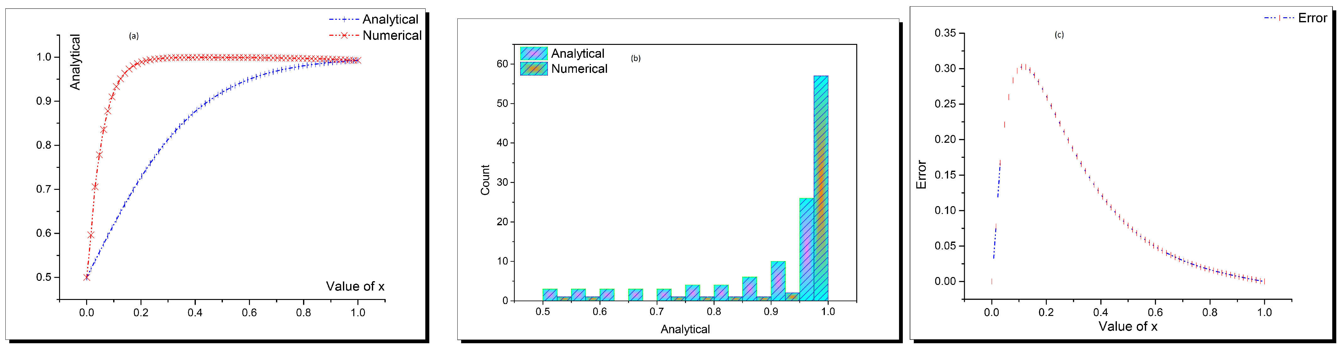
Value of x	Analytical	Numerical	Error	Value of x	Analytical	Numerical	Error
0	0.5	0.5	0	0.515625	0.925947	0.999254	0.073307
0.015625	0.519127	0.596515	0.077388	0.53125	0.931028	0.999203	0.068176
0.03125	0.538199	0.705602	0.167403	0.546875	0.935784	0.999146	0.063362
0.046875	0.557159	0.77828	0.221121	0.5625	0.940233	0.999082	0.058849
0.0625	0.575954	0.835791	0.259837	0.578125	0.944392	0.999013	0.05462
0.078125	0.594532	0.878033	0.283501	0.59375	0.948278	0.998936	0.050658
0.09375	0.612843	0.909745	0.296901	0.609375	0.951906	0.998854	0.046947
0.109375	0.630841	0.933241	0.3024	0.625	0.955292	0.998764	0.043472
0.125	0.648482	0.950674	0.302192	0.640625	0.95845	0.998667	0.040217
0.140625	0.665726	0.963567	0.297841	0.65625	0.961393	0.998561	0.037168
0.15625	0.682539	0.973094	0.290555	0.671875	0.964136	0.998448	0.034312
0.171875	0.698889	0.980124	0.281235	0.6875	0.966691	0.998325	0.031634
0.1875	0.714748	0.985307	0.270559	0.703125	0.96907	0.998192	0.029123
0.203125	0.730095	0.989125	0.25903	0.71875	0.971283	0.998049	0.026765
0.21875	0.744911	0.991936	0.247025	0.734375	0.973343	0.997894	0.024551
0.234375	0.759182	0.994003	0.234821	0.75	0.975259	0.997727	0.022468
0.25	0.772897	0.995521	0.222623	0.765625	0.97704	0.997547	0.020506
0.265625	0.786052	0.996634	0.210582	0.78125	0.978696	0.997352	0.018656
0.28125	0.798644	0.997448	0.198805	0.796875	0.980235	0.997142	0.016907
0.296875	0.810672	0.998042	0.18737	0.8125	0.981665	0.996915	0.015251
0.3125	0.822143	0.998474	0.176331	0.828125	0.982993	0.996671	0.013678
0.328125	0.833061	0.998784	0.165724	0.84375	0.984226	0.996407	0.012181
0.34375	0.843437	0.999006	0.155569	0.859375	0.985372	0.996122	0.010751
0.359375	0.853281	0.999161	0.14588	0.875	0.986435	0.995815	0.00938
0.375	0.862607	0.999267	0.13666	0.890625	0.987422	0.995484	0.008062
0.390625	0.87143	0.999336	0.127906	0.90625	0.988338	0.995126	0.006788
0.40625	0.879765	0.999377	0.119611	0.921875	0.989188	0.99474	0.005552
0.421875	0.88763	0.999396	0.111766	0.9375	0.989977	0.994326	0.004349
0.4375	0.895041	0.999399	0.104357	0.953125	0.990709	0.993871	0.003162
0.453125	0.902018	0.999388	0.09737	0.96875	0.991387	0.993411	0.002023
0.46875	0.908578	0.999367	0.090789	0.984375	0.992017	0.992795	0.000778
0.484375	0.914741	0.999337	0.084596	1	0.992601	0.992601	$5.55\times {10}^{-17}$

.

2.2. Kud Analytical vs. TQBS Numerical Techniques along (2+1) D-Fisher-KPP Model

Applying the MKud. scheme’s framework and its auxiliary $({\Gamma }^{\prime }{\left(\mathfrak{S}\right)=ln\left(k\right)(\Gamma \left(\mathfrak{S}\right)}^2$$-\Gamma \left(\mathfrak{S}\right)\left)\right)$ where k is an arbitrary constant to be determined later, to Equation (4), we obtain the following sets of the above-mentioned parameters:

Set I

$$\begin{array}{c}\hfill a_0=-1,a_1=2,r=2,\mu =-\frac{1}{{log}^2\left(k\right)}.\end{array}$$

Set II

$$\begin{array}{c}\hfill a_0=0,a_1=1,r=\frac{4log\left(k\right)-3}{2log\left(k\right)},\mu =-\frac{1}{4{log}^2\left(k\right)}.\end{array}$$

Set III

$$\begin{array}{c}\hfill a_0=1,a_1=-1,r=\frac{4log\left(k\right)+3}{2log\left(k\right)},\mu =-\frac{1}{4{log}^2\left(k\right)}.\end{array}$$

Therefore, the computational wave solutions of the (2+1) D-Fisher-KPP model are constructed in the following formulas:

$$\begin{array}{c}\hfill {\mathcal{S}}_{\mathrm{I}}(x,y,t)=\frac{2}{1\pm k^{2t+x+y}}-1,\end{array}$$

(28)

$$\begin{array}{c}\hfill {\mathcal{S}}_{\mathrm{II}}(x,y,t)=\frac{1}{1\pm k^{-\frac{3t}{2log\left(k\right)}+2t+x+y}},\end{array}$$

(29)

$$\begin{array}{c}\hfill {\mathcal{S}}_{\mathrm{III}}(x,y,t)=1-\frac{1}{1\pm k^{\frac{3t}{2log\left(k\right)}+2t+x+y}}.\end{array}$$

(30)

Semi-Analytical Solutions

Applying the TQBS numerical technique with the following initial condition $\mathcal{F}(x,0,0)=\frac{1}{e^x+1}$ gets the following shown analytical and numerical solutions’ values with respect to different values of x in

Table 2. Analytical and numerical matching along MKud. and TQBS techniques.

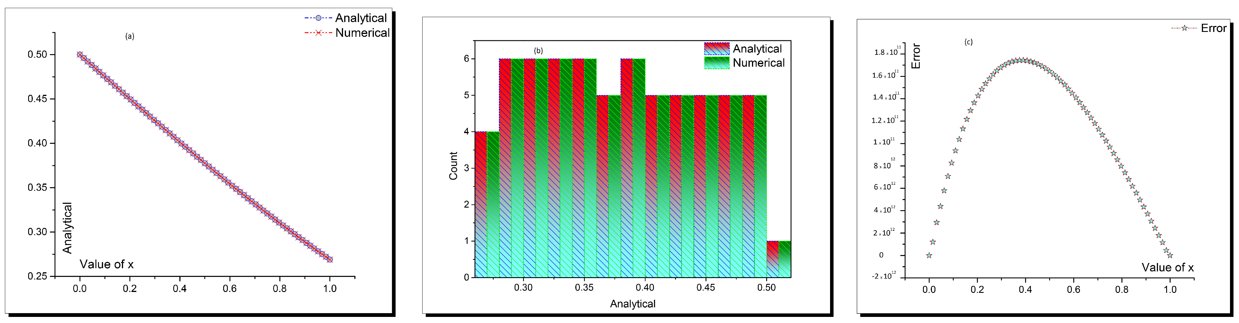
Value of x	Analytical	Numerical	Error	Value of x	Analytical	Numerical	Error
0	0.5	0.5	0	0.515625	0.373876	0.373876	1.62 $\times {10}^{-11}$
0.015625	0.496094	0.496094	1.2 $\times {10}^{-12}$	0.53125	0.370225	0.370225	1.59 $\times {10}^{-11}$
0.03125	0.492188	0.492188	2.94 $\times {10}^{-12}$	0.546875	0.36659	0.36659	1.56 $\times {10}^{-11}$
0.046875	0.488283	0.488283	4.39 $\times {10}^{-12}$	0.5625	0.362969	0.362969	1.52 $\times {10}^{-11}$
0.0625	0.48438	0.48438	5.79 $\times {10}^{-12}$	0.578125	0.359364	0.359364	1.49 $\times {10}^{-11}$
0.078125	0.480479	0.480479	7.07 $\times {10}^{-12}$	0.59375	0.355775	0.355775	1.45 $\times {10}^{-11}$
0.09375	0.47658	0.47658	8.26 $\times {10}^{-12}$	0.609375	0.352202	0.352202	1.41 $\times {10}^{-11}$
0.109375	0.472683	0.472683	9.37 $\times {10}^{-12}$	0.625	0.348645	0.348645	1.37 $\times {10}^{-11}$
0.125	0.468791	0.468791	1.04 $\times {10}^{-11}$	0.640625	0.345105	0.345105	1.32 $\times {10}^{-11}$
0.140625	0.464902	0.464902	1.13 $\times {10}^{-11}$	0.65625	0.341582	0.341582	1.28 $\times {10}^{-11}$
0.15625	0.461017	0.461017	1.22 $\times {10}^{-11}$	0.671875	0.338077	0.338077	1.23 $\times {10}^{-11}$
0.171875	0.457137	0.457137	1.29 $\times {10}^{-11}$	0.6875	0.334589	0.334589	1.18 $\times {10}^{-11}$
0.1875	0.453262	0.453262	1.36 $\times {10}^{-11}$	0.703125	0.33112	0.33112	1.13 $\times {10}^{-11}$
0.203125	0.449393	0.449393	1.43 $\times {10}^{-11}$	0.71875	0.327668	0.327668	1.08 $\times {10}^{-11}$
0.21875	0.44553	0.44553	1.48 $\times {10}^{-11}$	0.734375	0.324235	0.324235	1.02 $\times {10}^{-11}$
0.234375	0.441673	0.441673	1.53 $\times {10}^{-11}$	0.75	0.320821	0.320821	9.68 $\times {10}^{-12}$
0.25	0.437823	0.437823	1.58 $\times {10}^{-11}$	0.765625	0.317426	0.317426	9.13 $\times {10}^{-12}$
0.265625	0.433981	0.433981	1.62 $\times {10}^{-11}$	0.78125	0.314051	0.314051	8.56 $\times {10}^{-12}$
0.28125	0.430147	0.430147	1.65 $\times {10}^{-11}$	0.796875	0.310694	0.310694	7.98 $\times {10}^{-12}$
0.296875	0.426322	0.426322	1.68 $\times {10}^{-11}$	0.8125	0.307358	0.307358	7.39 $\times {10}^{-12}$
0.3125	0.422505	0.422505	1.7 $\times {10}^{-11}$	0.828125	0.304042	0.304042	6.8 $\times {10}^{-12}$
0.328125	0.418697	0.418697	1.72 $\times {10}^{-11}$	0.84375	0.300746	0.300746	6.19 $\times {10}^{-12}$
0.34375	0.414899	0.414899	1.73 $\times {10}^{-11}$	0.859375	0.29747	0.29747	5.58 $\times {10}^{-12}$
0.359375	0.411111	0.411111	1.74 $\times {10}^{-11}$	0.875	0.294215	0.294215	4.96 $\times {10}^{-12}$
0.375	0.407333	0.407333	1.74 $\times {10}^{-11}$	0.890625	0.290981	0.290981	4.34 $\times {10}^{-12}$
0.390625	0.403567	0.403567	1.74 $\times {10}^{-11}$	0.90625	0.287768	0.287768	3.71 $\times {10}^{-12}$
0.40625	0.399812	0.399812	1.74 $\times {10}^{-11}$	0.921875	0.284576	0.284576	3.07 $\times {10}^{-12}$
0.421875	0.396068	0.396068	1.73 $\times {10}^{-11}$	0.9375	0.281406	0.281406	2.44 $\times {10}^{-12}$
0.4375	0.392337	0.392337	1.72 $\times {10}^{-11}$	0.953125	0.278257	0.278257	1.79 $\times {10}^{-12}$
0.453125	0.388618	0.388618	1.71 $\times {10}^{-11}$	0.96875	0.27513	0.27513	1.16 $\times {10}^{-12}$
0.46875	0.384912	0.384912	1.69 $\times {10}^{-11}$	0.984375	0.272025	0.272025	4.57 $\times {10}^{-13}$
0.484375	0.38122	0.38122	1.67 $\times {10}^{-11}$	1	0.268941	0.268941	5.55 $\times {10}^{-17}$

.

3. Results’ Interpretation

This section studies the originality and novelty of this research paper. It also shows the accuracy of the obtained analytical solutions. The MDA and MKud. computational schemes have been applied to the (2+1) D-Fisher-KPP model for constructed novel analytical wave solutions. Many distinct analytical wave solutions have been obtained, and some of them have been demonstrated through sketches in 2D, 3D, and contour plots. These figures explain the dynamical characterization of the reaction–diffusion system by traveling waves in population genetics and propagating domain walls and pattern formation in bi-stable systems in nematic liquid crystals. Figure 1, Figure 2, Figure 3 and Figure 4 show some novel analytical wave solutions with different values to the above–mentioned parameters. Comparing our solutions with those that have been obtained in a previously published paper [17,41] shows our solutions are completely different from those that have been evaluated in [41]. Still, some of our solutions match the obtained solutions in [17] when $\alpha =1$, where in that paper, the authors in that paper studied the fractional form of the considered model.

The TQBS scheme has been applied to the considered model based on the obtained computational solutions. The absolute error between the analytical and numerical solutions has been calculated to show the accuracy of the obtained results and used methods (Table 1 and Table 2 and Figure 5 and Figure 6). This calculating shows the arrogance of the MKud. method over the MDA method, where its absolute values of error are much smaller than those obtained by the MDA method (Figure 7).

4. Conclusions

This research paper has successfully handled the nonlinear (2+1) D-Fisher-KPP model in population genetics and nematic liquid crystals through analytical and numerical investigations. The MDA, MKud., and TQBS schemes have been employed to find accurate novel analytical wave solutions of the considered model. Some obtained solutions have been represented in three different types of sketches. The accuracy of the MKud. method has been verified over the MDA method, where it is our fourth paper in keeping with the title’s accuracy on the computational schemes.

References

- Helliar, C.V.; Crawford, L.; Rocca, L.; Teodori, C.; Veneziani, M. Permissionless and permissioned blockchain diffusion. Int. J. Inf. Manag. 2020, 54, 102136. [Google Scholar] [CrossRef]
- Axpe, E.; Chan, D.; Offeddu, G.S.; Chang, Y.; Merida, D.; Hernandez, H.L.; Appel, E.A. A multiscale model for solute diffusion in hydrogels. Macromolecules 2019, 52, 6889–6897. [Google Scholar] [CrossRef] [Green Version]
- Chandrabose, S.; Chen, K.; Barker, A.J.; Sutton, J.J.; Prasad, S.K.; Zhu, J.; Zhou, J.; Gordon, K.C.; Xie, Z.; Zhan, X.; et al. High exciton diffusion coefficients in fused ring electron acceptor films. J. Am. Chem. Soc. 2019, 141, 6922–6929. [Google Scholar] [CrossRef]
- Grebenkov, D.S. Paradigm shift in diffusion-mediated surface phenomena. Phys. Rev. Lett. 2020, 125, 078102. [Google Scholar] [CrossRef] [PubMed]
- Iima, M.; Honda, M.; Sigmund, E.E.; Ohno Kishimoto, A.; Kataoka, M.; Togashi, K. Diffusion MRI of the breast: Current status and future directions. J. Magn. Reson. Imaging 2020, 52, 70–90. [Google Scholar] [CrossRef] [PubMed]
- Brown, J.L.; Johnston, W.; Delaney, C.; Rajendran, R.; Butcher, J.; Khan, S.; Bradshaw, D.; Ramage, G.; Culshaw, S. Biofilm-stimulated epithelium modulates the inflammatory responses in co-cultured immune cells. Sci. Rep. 2019, 9, 1–14. [Google Scholar] [CrossRef] [PubMed] [Green Version]
- Hosseininia, M.; Heydari, M. Legendre wavelets for the numerical solution of nonlinear variable-order time fractional 2D reaction–diffusion equation involving Mittag–Leffler non-singular kernel. Chaos Solitons Fractals 2019, 127, 400–407. [Google Scholar] [CrossRef]
- García-Crespo, C.; Soria, M.E.; Gallego, I.; Ávila, A.I.d.; Martínez-González, B.; Vázquez-Sirvent, L.; Gómez, J.; Briones, C.; Gregori, J.; Quer, J.; et al. Dissimilar conservation pattern in hepatitis C virus mutant spectra, consensus sequences, and data banks. J. Clin. Med. 2020, 9, 3450. [Google Scholar] [CrossRef]
- Yang, X.; Li, Y.; Zou, L.; Zhu, Z. Role of exosomes in crosstalk between cancer-associated fibroblasts and cancer cells. Front. Oncol. 2019, 9, 356. [Google Scholar] [CrossRef] [PubMed]
- Bochner, S. Diffusion equation and stochastic processes. Proc. Natl. Acad. Sci. USA 1949, 35, 368. [Google Scholar] [CrossRef] [Green Version]
- Elphick, C.; Coullet, P.; Repaux, D. Nature of spatial chaos. Phys. Rev. Lett 1987, 58, 431–434. [Google Scholar]
- Dee, G.; van Saarloos, W. Bistable systems with propagating fronts leading to pattern formation. Phys. Rev. Lett. 1988, 60, 2641. [Google Scholar] [CrossRef] [Green Version]
- Van Saarloos, W. Front propagation into unstable states. II. Linear versus nonlinear marginal stability and rate of convergence. Phys. Rev. A 1989, 39, 6367. [Google Scholar] [CrossRef]
- El-Hachem, M.; McCue, S.W.; Jin, W.; Du, Y.; Simpson, M.J. Revisiting the Fisher–Kolmogorov–Petrovsky–Piskunov equation to interpret the spreading–extinction dichotomy. Proc. R. Soc. A 2019, 475, 20190378. [Google Scholar] [CrossRef] [Green Version]
- Fisher, R.A. The wave of advance of advantageous genes. Ann. Eugen. 1937, 7, 355–369. [Google Scholar] [CrossRef] [Green Version]
- Kolmogorov, A.N.; Petrovskii, I.G.; Piskunov, N.S. A study of the diffusion equation with increase in the amount of substance and its application to a biology problem. Bull. Univ. Mosc. Ser. Int. 1937, 1, 1–16. [Google Scholar]
- Veeresha, P.; Prakasha, D.; Singh, J.; Khan, I.; Kumar, D. Analytical approach for fractional extended Fisher–Kolmogorov equation with Mittag-Leffler kernel. Adv. Differ. Equ. 2020, 2020, 1–17. [Google Scholar] [CrossRef]
- Levchenko, E.A.; Shapovalov, A.V.; Trifonov, A.Y. Symmetries of the Fisher–Kolmogorov–Petrovskii–Piskunov equation with a nonlocal nonlinearity in a semiclassical approximation. J. Math. Anal. Appl. 2012, 395, 716–726. [Google Scholar] [CrossRef] [Green Version]
- Luther, R. II. Sitzung am Dienstag, den 22. Mai, vormittags 9 Uhr, im grossen Auditorium des chemischen Laboratoriums der Technischen Hochschule. Räumliche Fortpflanzung chemischer Reaktionen. Z. Elektrochem. Angew. Phys. Chem. 1906, 12, 596–600. [Google Scholar] [CrossRef]
- Oruç, Ö. An efficient wavelet collocation method for nonlinear two-space dimensional Fisher–Kolmogorov–Petrovsky–Piscounov equation and two-space dimensional extended Fisher–Kolmogorov equation. Eng. Comput. 2020, 36, 839–856. [Google Scholar] [CrossRef]
- Morgado, G.; Nowakowski, B.; Lemarchand, A. Fisher-Kolmogorov-Petrovskii-Piskunov wave front as a sensor of perturbed diffusion in concentrated systems. Phys. Rev. E 2019, 99, 022205. [Google Scholar] [CrossRef] [Green Version]
- El-Nabulsi, R.A. Fourth-Order Ginzburg-Landau differential equation a la Fisher-Kolmogorov and quantum aspects of superconductivity. Phys. C Supercond. Its Appl. 2019, 567, 1353545. [Google Scholar] [CrossRef]
- El-Nabulsi, R.A. Orbital dynamics satisfying the 4 th-order stationary extended Fisher-Kolmogorov equation. Astrodynamics 2020, 4, 31–39. [Google Scholar] [CrossRef]
- Khater, M.M.; Seadawy, A.R.; Lu, D. Bifurcations of solitary wave solutions for (two and three)-dimensional nonlinear partial differential equation in quantum and magnetized plasma by using two different methods. Results Phys. 2018, 9, 142–150. [Google Scholar] [CrossRef]
- Khater, M.; Attia, R.A.; Abdel-Aty, A.H.; Abdel-Khalek, S.; Al-Hadeethi, Y.; Lu, D. On the computational and numerical solutions of the transmission of nerve impulses of an excitable system (the neuron system). J. Intell. Fuzzy Syst. 2020, 38, 2603–2610. [Google Scholar] [CrossRef]
- Qin, H.; Attia, R.A.; Khater, M.; Lu, D. Ample soliton waves for the crystal lattice formation of the conformable time-fractional (N+ 1) Sinh-Gordon equation by the modified Khater method and the Painlevé property. J. Intell. Fuzzy Syst. 2020, 38, 2745–2752. [Google Scholar] [CrossRef]
- Khater, M.M.; Baleanu, D. On abundant new solutions of two fractional complex models. Adv. Differ. Equ. 2020, 2020, 1–14. [Google Scholar] [CrossRef]
- Yue, C.; Khater, M.M.; Attia, R.A.; Lu, D. The plethora of explicit solutions of the fractional KS equation through liquid–gas bubbles mix under the thermodynamic conditions via Atangana–Baleanu derivative operator. Adv. Differ. Equ. 2020, 2020, 1–12. [Google Scholar] [CrossRef] [Green Version]
- Abdel-Aty, A.H.; Khater, M.M.; Dutta, H.; Bouslimi, J.; Omri, M. Computational solutions of the HIV-1 infection of CD4+ T-cells fractional mathematical model that causes acquired immunodeficiency syndrome (AIDS) with the effect of antiviral drug therapy. Chaos Solitons Fractals 2020, 139, 110092. [Google Scholar] [CrossRef] [PubMed]
- Khater, M.M.; Attia, R.A.; Park, C.; Lu, D. On the numerical investigation of the interaction in plasma between (high & low) frequency of (Langmuir & ion-acoustic) waves. Results Phys. 2020, 18, 103317. [Google Scholar]
- Khater, M.M.; Attia, R.A.; Abdel-Aty, A.H.; Alharbi, W.; Lu, D. Abundant analytical and numerical solutions of the fractional microbiological densities model in bacteria cell as a result of diffusion mechanisms. Chaos Solitons Fractals 2020, 136, 109824. [Google Scholar] [CrossRef]
- Abdel-Aty, A.H.; Khater, M.M.; Attia, R.A.; Abdel-Aty, M.; Eleuch, H. On the new explicit solutions of the fractional nonlinear space-time nuclear model. Fractals 2020, 28, 2040035. [Google Scholar] [CrossRef]
- Qin, H.; Khater, M.; Attia, R.A. Inelastic Interaction and Blowup New Solutions of Nonlinear and Dispersive Long Gravity Waves. J. Funct. Spaces 2020, 2020, 5362989. [Google Scholar] [CrossRef]
- Park, C.; Khater, M.M.; Abdel-Aty, A.H.; Attia, R.A.; Rezazadeh, H.; Zidan, A.; Mohamed, A.B. Dynamical analysis of the nonlinear complex fractional emerging telecommunication model with higher–order dispersive cubic–quintic. Alex. Eng. J. 2020, 59, 1425–1433. [Google Scholar] [CrossRef]
- Khater, M.M.; Ghanbari, B.; Nisar, K.S.; Kumar, D. Novel exact solutions of the fractional Bogoyavlensky–Konopelchenko equation involving the Atangana-Baleanu-Riemann derivative. Alex. Eng. J. 2020, 59, 2957–2967. [Google Scholar] [CrossRef]
- Yue, C.; Lu, D.; Khater, M.M.; Abdel-Aty, A.H.; Alharbi, W.; Attia, R.A. On explicit wave solutions of the fractional nonlinear DSW system via the modified Khater method. Fractals 2020, 28, 2040034. [Google Scholar] [CrossRef]
- Abdel-Aty, A.H.; Khater, M.; Attia, R.A.; Eleuch, H. Exact Traveling and Nano-Solitons Wave Solitons of the Ionic Waves Propagating along Microtubules in Living Cells. Mathematics 2020, 8, 697. [Google Scholar] [CrossRef]
- Qin, H.; Khater, M.; Attia, R.A. Copious Closed Forms of Solutions for the Fractional Nonlinear Longitudinal Strain Wave Equation in Microstructured Solids. Math. Probl. Eng. 2020, 2020, 3498796. [Google Scholar] [CrossRef]
- Demiray, S.T.; Bayrakci, U. Soliton solutions for space-time fractional Heisenberg ferromagnetic spin chain equation by generalized Kudryashov method and modified exp-expansion function method. Rev. Mex. Física 2021, 67, 393–402. [Google Scholar] [CrossRef]
- Chu, Y.; Khater, M.M.; Hamed, Y. Diverse novel analytical and semi-analytical wave solutions of the generalized (2+1)-dimensional shallow water waves model. AIP Adv. 2021, 11, 015223. [Google Scholar] [CrossRef]
- Shakeel, M. Travelling wave solution of the Fisher-Kolmogorov equation with non-linear diffusion. Appl. Math. 2013, 4, 35319. [Google Scholar] [CrossRef]