A Multispecies Cross-Diffusion Model for Territorial Development

Abstract

We develop an agent-based model on a lattice to investigate territorial development motivated by markings such as graffiti, generalizing a previously-published model to account for K groups instead of two groups. We then analyze this model and present two novel variations. Our model assumes that agents’ movement is a biased random walk away from rival groups’ markings. All interactions between agents are indirect, mediated through the markings. We numerically demonstrate that in a system of three groups, the groups segregate in certain parameter regimes. Starting from the discrete model, we formally derive the continuum system of $2K$ convection–diffusion equations for our model. These equations exhibit cross-diffusion due to the avoidance of the rival groups’ markings. Both through numerical simulations and through a linear stability analysis of the continuum system, we find that many of the same properties hold for the K-group model as for the two-group model. We then introduce two novel variations of the agent-based model, one corresponding to some groups being more timid than others, and the other corresponding to some groups being more threatening than others. These variations present different territorial patterns than those found in the original model. We derive corresponding systems of convection–diffusion equations for each of these variations, finding both numerically and through linear stability analysis that each variation exhibits a phase transition.

1. Introduction

Many types of organisms are known to exhibit territoriality. Examples include insects, fish, amphibians, reptiles, birds, mammals [1], and, of course, human beings [2]. Even plants could be considered to display this trait [3], with some such as Eucalyptus excreting a chemical that inhibits the growth of other species [4]. Reasons for territorial behavior include protection of breeding sites and access to resources, and territorial organisms have several ways of claiming their territory. Two common ways are through some sort of marking, either chemical or physical, and through direct confrontation.

In this paper, we focus on the case of territory formation for a mobile species through territorial markings. We use the example of gangs of human beings reacting to the graffiti of other gangs, though the model could also be applied to other mobile species. In [5,6], Moorcroft et al. modeled how different packs of animals like coyotes and wolves base their movement on scent marking. It was discovered that both coyotes and wolves use scent marking to tag territories [7]. Once wolves or coyotes encounter foreign scents, they in turn mark their territory with their scent and usually head back to their own home territory. This dynamic was studied in detail in [8], where it was found that different packs of wolves can live in the same region without having contact with other packs, but each has its own territory.

More recently, advances have been made in the field of movement ecology with models of territorial development motivated by scent marking, many exhibiting cross-diffusion. Some, such as those in [9], are similar to the continuum systems derived in [10] and in Section 1.1–Section 3.2 of the current work, though there are several subtle but important differences. The interested reader is referred to [9,11,12], which provide an excellent overview of the current state of this ecological literature and important new results for cross-diffusion models in spatial population dynamics. Our work here provides a mechanistic underpinning for this type of PDE model, along with the formal derivation of convection–diffusion systems. Section 5 also offers two novel variations, which can be adapted to particular species and ecological situations.

Researchers studying gang dynamics have based the gang movement dynamics on existing ecological models of animal species that exhibit territorial behavior. Gangs have distinctive graffiti and other special identifiers, such as handshakes and tattoos, to distinguish themselves from other gangs [13,14]. In addition, it is found that in major cities around the world, gangs claim territory by marking it with graffiti, and gangs tend to avoid territory claimed by other gangs unless they are actively seeking out retaliation [15,16]. Smith et al. [17] combined the ecological model in [6] with Hegemann et al.’s network model [18] to produce a model for gang territoriality. The new model was then solved numerically, and their results were compared to real data about gang territories in Los Angeles. In [19], Barbaro et al. used a statistical mechanics approach to study how gang territories could be formed based on graffiti. This also drew on ideas from coyote and wolf scent-marking. The authors chose to use a spin system similar to the Ising model [20] that simulates ferromagnetism. A two-dimensional lattice was used, with an agent and a graffiti spin at each site, and there were only indirect interactions between the agent spins. The authors showed that their model exhibits a phase transition in which gangs cluster together to form territory.

Other work on modeling criminal behavior has also been done. This work is tangential to the work presented here, but is summarized for the interested reader. Clustering methods have been used to study gang affiliations between gang members in Los Angeles [21]. Network models are also used to study gangs. In [18], the authors present an agent-based model, which is coupled with a rivalry network to explore how gang rivalries are formed. In [22], a model for burglary was developed, and a continuum system consisting of coupled reaction–diffusion equations was derived. This and similar systems were analyzed in [23,24,25]. Modifications of the model were explored in [26,27]. The reaction–diffusion equations were analyzed further in [28], which showed that they exhibit similar behavior to chemotactic systems with cross-diffusion. Recently, in [29], Wang et al. extended the burglary model by including independent Poisson clocks in the time steps; a martingale with both a deterministic and a stochastic part was derived and analyzed. Work on riots and social segregation have also followed from this line of research [30,31]. For a more in-depth review of the crime modeling literature, the reader is referred to [32].

Our paper is based on the work of [10], wherein the authors performed a bottom-up approach similar to the Moorcroft model [6], producing a discrete system to describe gang territorial development and formally deriving from it the following system of convection–diffusion equations:

$$\left\{\begin{array}{c}{\displaystyle \frac{\partial {\xi }_A}{\partial t}(x,y,t)=\gamma {\rho }_A(x,y,t)-\lambda {\xi }_A(x,y,t)}\hfill \\ {\displaystyle \frac{\partial {\xi }_B}{\partial t}(x,y,t)=\gamma {\rho }_B(x,y,t)-\lambda {\xi }_B(x,y,t)}\hfill \\ {\displaystyle \frac{\partial {\rho }_A}{\partial t}(x,y,t)=\frac{D}{4}\nabla ·\left[\nabla {\rho }_A(x,y,t)+2\beta \left({\rho }_A(x,y,t)\nabla {\xi }_B(x,y,t)\right)\right]}\hfill \\ {\displaystyle \frac{\partial {\rho }_B}{\partial t}(x,y,t)=\frac{D}{4}\nabla ·\left[\nabla {\rho }_B(x,y,t)+2\beta \left({\rho }_B(x,y,t)\nabla {\xi }_A(x,y,t)\right)\right],}\hfill \end{array}\right.$$

(1)

where ${\xi }_i$ is the graffiti density of gang i and ${\rho }_i$ is the agent density from gang i. The model undergoes a phase transition from no territorial development to distinct territorial formation as the parameter $\beta$ is changed. This phase transition was found both at the discrete and continuum level. The authors consider only the case of two gangs. A modified version of the convection–diffusion system in [10] was analyzed in [33], where they proved a weak stability result and identified equilibrium solutions; interestingly, though, they did not find segregated equilibrium solutions in this modified system.

In this paper, we generalize the model and results of [10] to consider any finite number K of groups. This is important, because it gives the model much more flexibility. Often when considering territorial formation, there are more than two groups involved. We define a lattice model with K groups, each of whom tries to avoid the graffiti of the other groups. We neglect births and deaths, considering instead fixed population sizes in each gang, so that any losses of population are compensated by gains. This is reasonable, since we would not expect the size of the gangs to change significantly over the course of time that we simulate the territorial dynamics. The birth and death neglect is in line with other territorial ecological models that concentrate on short term movement where the individual response is faster than the population changes [9,12]. We work on a periodic lattice, which we think of as tiling a very large or infinite space, since we do not have specific geographic constraints in mind. We also assume that all agents move to a neighboring lattice site at every time step for simplicity, since this will help in the derivation of the continuum limits. As in the two-gang model, we observe that our model undergoes a phase transition, and we numerically examine the phase transition and how it is affected by changing our spatial discretization. We then follow [10] in deriving a continuum system. We perform a two-dimensional linear stability analysis to identify the critical parameter, showing that above the bifurcation value of $\beta$ all wave numbers are unstable, in agreement with the observed behavior of the discrete model. We then explore two variations of the model, where we allow each group to have a different $\beta$ value. In the first variation, called the Timidity Model, this $\beta$ affects the strength with which they avoid other groups’ graffiti. In the second, called the Threat Level Model, a group’s $\beta$ value affects how strongly other groups avoid their graffiti. We derive corresponding continuum systems of both models, and find the critical value at which the behavior changes from well-mixed groups to segregated groups in the case of two groups. This also gives us an intuition to the critical parameter for K groups, both in the variations and the original model, which we numerically validate in the three group case.

This paper is a significant contribution both to the field of movement ecology and to the mathematical literature. We derive three discrete models for an arbitrary number of groups, each assuming different motivations and each showing distinct territorial dynamics. We also derive three novel systems of convection–diffusion equations exhibiting cross-diffusion, where the only interaction between groups occurs between agents and the markings of groups other than their own. Furthermore, we find the critical parameters for the transition between well-mixed and segregated territories for all three models we introduce for two groups, with a proposed formula for K groups.

This paper’s outline is as follows: In Section 1.1, we introduce our extension of the original two-gang agent-based model [10]. The rest of the article is based upon this extension. We next define an order parameter in Section 1.2 that will be used to analyze our system’s different states and characterize phase transitions. In Section 2, we present the results of a special case of our discrete model numerical simulations as well as show our analysis of the systems’ phase transitions. In Section 3.1 and Section 3.2, we will derive the general continuum limit from the discrete model. In Section 3.3 and Section 4, we will derive a steady-state solution for our continuum model and perform linear stability analysis to determine whenever the well-mixed solution becomes unstable. In Section 5, we introduce and study two variations on the model, where parameter $\beta$ is made gang-dependent. Finally, in Section 6, we conclude with a discussion of the results and open problems.

1.1. Discrete Model

In this paper, we extend and generalize the interacting particle model in [10] to now include K gangs as opposed to only two, keeping all other dynamics similar. We shall use a square lattice S with area 1 and grid discretization $L\times L$, with periodic boundary conditions. Since the lattice length is assumed to be equal to one, and L is a dimensionless quantity that represents the number of lattice sites, $l=\frac{1}{L}$ is the lattice spacing with units of length.

We assume that we have K gangs, $1,2,\cdots K$, and the number of agents belonging in each gang j is denoted by $N_j$. The systems’ total number of agents is denoted by N:

$$N=\sum _{i=1}^K{N}_i.$$

These agents are distributed over the lattice. Our model allows multiple gang agents regardless of their gang affiliation to be on the same site. We denote the number of agents of gang j at site $(x,y)$ at time t by $n_j(x,y,t)$ and their densities are ${\rho }_j(x,y,t)=\frac{n_j(x,y,t)}{l^2}$, where $l=\frac{1}{L}$ is the lattice spacing. The amount of graffiti belonging to gang j at site $(x,y)$ on time t is denoted by $g_j(x,y,t)$. We denote the graffiti density of gang j by ${\xi }_j(x,y,t)=\frac{g_j(x,y,t)}{l^2}$.

Our model assumes that every agent moves at every time step to one of their four neighboring sites, which are the sites up, down, to the left, and to the right of it. That is, an agent currently occupying site $(x,y)$ would move to an element of the set of sites $\left\{\right(x+l,y),(x-l,y),(x,y+l),(x,y-l\left)\right\}$. The neighboring sites of $(x,y)$ will be denoted by $(\tilde{x},\tilde{y})\sim (x,y)$. In our model, each agent performs a biased random walk, trying to avoid the opposing gangs graffiti. Following [10], our model assumes that every agent has some probability of putting down its own gang’s graffiti on the lattice and this graffiti discourages the movement of agents from a different gang onto that lattice site. However, now that we are considering more than two gangs, each gang must avoid the graffiti of all other gangs, leading us to define the opposition sum for gang j at site $(x,y)$ at time t:

$${\psi }_j(x,y,t):=\sum _{\begin{array}{c}i=1\\ i\ne j\end{array}}^K{\xi }_i(x,y,t).$$

(2)

We use this opposition sum to inform the movement dynamics of the agents. The movement from site $s_1=(x_1,y_1)\in S$ to a neighboring site $s_2(x_2,y_2)\in S$ at time t is denoted by $(x_1\to x_2,y_1\to y_2,t)$. Here, the symbol → represents the change of spatial coordinates at time t. The probability of an agent from gang j to move from site $(x_1,y_1)\in S$ to one of the neighboring sites $(x_2,y_2)$ is defined to be

$$M_j(x_1\to x_2,y_1\to y_2,t)=\frac{e^{-\beta {\psi }_j(x_2,y_2,t)}}{{\displaystyle \sum _{(\tilde{x},\tilde{y})\sim (x_1,y_1)}}{e}^{-\beta {\psi }_j(\tilde{x},\tilde{y},t)}},$$

(3)

again defined analogously to [10]. Here, the parameter $\beta$ encodes the strength of the avoidance of other gangs’ graffiti. As our model assumes that all of the agents must move at each time step, it is easily seen that

$$\sum _{(\tilde{x},\tilde{y})\sim (x,y)}{M}_j(x\to \tilde{x},y\to \tilde{y},t)=1.$$

(4)

The expected density of gang j is therefore

$$\begin{array}{cc}\hfill {\rho }_j(x,y,t+\delta t)=& {\rho }_j(x,y,t)+\sum _{(\tilde{x},\tilde{y})\sim (x,y)}{\rho }_A(\tilde{x},\tilde{y},t)M_j(\tilde{x}\to x,\tilde{y}\to y,t)\hfill \\ \hfill & -{\rho }_j(x,y,t)\sum _{(\tilde{x},\tilde{y})\sim (x,y)}{M}_j(x\to \tilde{x},y\to \tilde{y},t)\hfill \\ \hfill & =\sum _{(\tilde{x},\tilde{y})\sim (x,y)}{\rho }_A(\tilde{x},\tilde{y},t)M_j(\tilde{x}\to x,\tilde{y}\to y,t).\hfill \end{array}$$

(5)

For the graffiti density update rules, each agent adds graffiti at its current site with probability $\gamma$. It is also assumed that the graffiti decays at every site with a rate of $\lambda$. Both the graffiti addition and decay are scaled by the time step $\delta t$. Therefore, the graffiti density at site $(x,y)\in S$ at time $t+\delta t$ is

$${\xi }_j(x,y,t+\delta t)={\xi }_j(x,y,t)-\left(\delta t·\lambda \right){\xi }_j(x,y,t)+\left(\delta t·\gamma \right){\rho }_j(x,y,t).$$

(6)

In all of our simulations, we initially randomly distribute the agents’ locations using the multivariate uniform distribution on the lattice S. We also assume that the lattice is initially empty of graffiti.

1.2. Phases and an Order Parameter

In our simulations, we shall observe two phases, the well-mixed phase and the segregated phase. These phases, we will see, are determined by parameter $\beta$, introduced in (3). In the well-mixed phase, the agents are distributed randomly throughout the lattice and their movement approximates a random walk. However, for the segregated phase, the agents’ movement is a biased random walk, and the agents form territories by clustering together. In this Section, we shall define an order parameter and use it to quantify these different phases.

1.2.1. Expected Agent Density

We first compute the expected agent density for the well-mixed state at site $(x,y)$ for each gang j. In this phase, the agents from each gang are uniformly spread over the whole lattice S. Thus, the expected agent density for gang j at any given site is:

$$\begin{array}{cc}\hfill E\left({\rho }_j\right)& =\sum _{(x,y)\in S}{\rho }_j(x,y)\times \frac{1}{L^2}\hfill \\ \hfill & =\sum _{(x,y)\in S}\frac{n_j(x,y)}{l^2}\times \frac{1}{L^2}\hfill \\ \hfill & =\sum _{(x,y)\in S}{n}_j(x,y)\hfill \\ \hfill & =N_j.\hfill \end{array}$$

(7)

For the segregated phase, the agents are entirely separated into different territories, each occupied by a distinct gang. To determine the expected agent density for the segregated phase, we will need the following definitions and assumptions. We define the territory $S_j$ to be the set of all sites that are dominated by gang j agents, i.e., all sites that have more gang j agents than agents of another type. We also note that $S_j$ need not be connected. We also define the number of grid sites in sublattice $S_j$ by $R_j$, which is the number of sites dominated by gang j. We note that $R_j$ has the same units as $L^2$, which is dimensionless. We assume that the agents from each gang are uniformly distributed in their territory, and that all sites are occupied by agents; hence, every site is assumed to contain agents from exactly one gang. These assumptions are validated in our simulation in Section 2. Accordingly, ${\left\{S_j\right\}}_{j=1}^K$ form a partition for the lattice S for $j=1,2,\cdots ,K$.

Under these assumptions, we now calculate the expected agent density for the agent density for gang j in the segregated state by splitting the lattice S into two disjoint territories, $S_j$ and its complement ${S_j}^c$. Calculating the expected agent density within the complement of gang j′s territory easily finds:

$$\begin{array}{cc}\hfill E\left({\rho }_j\right)& =\sum _{(x,y)\in {S_j}^c}\frac{{\rho }_j(x,y)}{{R_j}^c}=0.\hfill \end{array}$$

This last equality follows because all agents for gang j are assumed to be in $S_j$ in the (perfectly) segregated phase, hence none are in ${S_j}^c$. Next, calculating the expected agent density within $S_j$ gives us:

$$\begin{array}{cc}\hfill E\left({\rho }_j\right)& =\sum _{(x,y)\in S_j}\frac{{\rho }_j(x,y)}{R_j}\hfill \\ \hfill & =\sum _{(x,y)\in S_j}\frac{n_j(x,y)}{l^2\times R_j}\hfill \\ \hfill & =\frac{N_j}{l^2{R}_j}.\hfill \end{array}$$

Thus, the expected agents density within $S_j$ is

$$\begin{array}{cc}\hfill E\left({\rho }_j(x,y)\right)& =\left\{\begin{array}{cc}\frac{N_j}{l^2{R}_j},\hfill & (x,y)\in S_j\hfill \\ 0,\hfill & (x,y)\in {S_j}^c.\hfill \end{array}\right.\hfill \end{array}$$

(8)

If we further assume that the areas dominated by each gang are almost equal and that there are an equal number of agents in each gang, we deduce that $R_j=\frac{L^2}{K}$, where K is the number of gangs. Under these assumptions, the expected density in a segregated state for an agent from gang j is

$$\begin{array}{cc}\hfill E\left({\rho }_j(x,y)\right)& =\left\{\begin{array}{cc}\frac{N_j}{l^2{R}_j},\hfill & (x,y)\in S_j\hfill \\ 0,\hfill & (x,y)\in {S_j}^c\hfill \end{array}\right.\hfill \\ \hfill & =\left\{\begin{array}{cc}K{N}_j,\hfill & (x,y)\in S_j\hfill \\ 0,\hfill & (x,y)\in {S_j}^c.\hfill \end{array}\right.\hfill \end{array}$$

1.2.2. An Order Parameter

To investigate the phase transition, we define the following order parameter:

$$\begin{array}{cc}\hfill \mathcal{E}\left(t\right)=\frac{1}{4(K-1)}{\left(\frac{1}{LN}\right)}^2\sum _{j=1}^K\sum _{i>j}^K\sum _{(x,y)\in S}\sum _{(\tilde{x},\tilde{y})\sim (x,y)}& |\left({\rho }_j(x,y,t)-{\rho }_i(x,y,t)\right)\times \hfill \\ \hfill & \left({\rho }_j(\tilde{x},\tilde{y},t)-{\rho }_i(\tilde{x},\tilde{y},t)\right)|.\hfill \end{array}$$

(9)

This order parameter is modeled after the order parameter in [10] and the Hamiltonian function for the Ising Model [20,34]. In terms of our model, our order parameter becomes more positive if a site and its neighbors are dominated by the same gang and becomes extremely small when a site and its neighbors are dominated by different gangs. It is approximately zero if the agents are well-mixed and none of the gangs are dominating territory.

This is due to the fact that in the segregated phase, the agents cluster together and this leads to there being only one gang present at site $(x,y)$. This makes the term inside the sum in Equation (9) to have a large magnitude; if the same is true at the neighboring site, the second term inside the sum is identical and once we multiply the two together, the resulting value would be a positive number. Thus, the order parameter should attain its maximum when the system is perfectly segregated. However, whenever agents from all gangs become uniformly distributed throughout the lattice, the result is that the two sets of parenthesis tend to be extremely small and close to zero. After summing over the whole lattice and all the gangs, the order parameter ends up near zero. Thus, the order parameter should attain its minimum value when the system is completely well-mixed.

We now calculate an approximation for the order parameter when the phases are well-mixed and when they are perfectly segregated. For simplicity, in this subsection and all of our simulations, we consider the special case of three gangs and we assume that the number of agents in each gang is equal, so that $N_j=\frac{N}{3}$ for j in $\{1,2,3\}$. The order parameter for this special case is

$$\begin{array}{cc}\hfill \mathcal{E}=\frac{1}{8}{\left(\frac{1}{LN}\right)}^2\sum _{(x,y)\in S}\sum _{(\tilde{x},\tilde{y})\sim (x,y)}& \left|\left({\rho }_1(x,y)-{\rho }_2(x,y)\right)\left({\rho }_1(\tilde{x},\tilde{y})-{\rho }_2(\tilde{x},\tilde{y})\right)\right|\hfill \\ \hfill +& \left|\left({\rho }_1(x,y)-{\rho }_3(x,y)\right)\left({\rho }_1(\tilde{x},\tilde{y})-{\rho }_3(\tilde{x},\tilde{y})\right)\right|\hfill \\ \hfill +& \left|\left({\rho }_2(x,y)-{\rho }_3(x,y)\right)\left({\rho }_2(\tilde{x},\tilde{y})-{\rho }_3(\tilde{x},\tilde{y})\right)\right|.\hfill \end{array}$$

(10)

In the well-mixed state, based on Equation (7) and on our assumptions that the agents from all gangs are uniformly distributed and that each lattice site has four neighbors, our equation simplifies to

$$\begin{array}{cc}\hfill \mathcal{E}=\frac{1}{8}{\left(\frac{1}{LN}\right)}^2\sum _{(x,y)\in S}& \left|4\left(N_1-N_2\right)\left(N_1-N_2\right)\right|+\left|4\left(N_1-N_3\right)\left(N_1-N_3\right)\right|\hfill \\ \hfill +& \left|4\left(N_2-N_3\right)\left(N_2-N_3\right)\right|.\hfill \end{array}$$

Simplifying the terms in the brackets yields that

$$\begin{array}{cc}\hfill \mathcal{E}& =\frac{4}{8}{\left(\frac{1}{LN}\right)}^2\sum _{(x,y)\in S}[{\left(N_1-N_2\right)}^2+{\left(N_1-N_3\right)}^2+{\left(N_2-N_3\right)}^2]\hfill \\ \hfill & =\frac{1}{2}{\left(\frac{1}{N}\right)}^2[{\left(N_1-N_2\right)}^2+{\left(N_1-N_3\right)}^2+{\left(N_2-N_3\right)}^2].\hfill \end{array}$$

However, since we assumed that the number of agents from each gang $N_1,N_2,$ and $N_3$ are equal, it follows easily that the order parameter for the agents in a well-mixed phase is

$$\mathcal{E}\approx 0.$$

(11)

We will next calculate the order parameter for the segregated phase. Here, we assume a perfectly segregated phase and split the lattice S into the three regions $S_1$, $S_2$ and $S_3$ belonging to each gang, which gives us:

$$\begin{array}{cc}\hfill \mathcal{E}=\frac{1}{8}{\left(\frac{1}{LN}\right)}^2[\sum _{j=1}^3\sum _{i>j}^3\sum _{\begin{array}{c}(x,y)\in S_k\\ k\in \{1,2,3\}\end{array}}\sum _{(\tilde{x},\tilde{y})\sim (x,y)}|& \left({\rho }_j(x,y)-{\rho }_i(x,y)\right)\left({\rho }_j(\tilde{x},\tilde{y})-{\rho }_i(\tilde{x},\tilde{y})\right)\left|\right].\hfill \end{array}$$

Using Equation (8), we substitute the expectation of each ${\rho }_i$ for each region, which gives us the following approximation:

$$\begin{array}{cc}\hfill \mathcal{E}\approx \frac{1}{8}{\left(\frac{1}{LN}\right)}^2[& \sum _{(x,y)\in S_1}[4{\left(\frac{N_1}{l^2{R}_1}\right)}^2+4{\left(\frac{N_1}{l^2{R}_1}\right)}^2]\hfill \\ \hfill +& \sum _{(x,y)\in S_2}[4{\left(\frac{-N_2}{l^2{R}_2}\right)}^2+4{\left(\frac{N_2}{l^2{R}_2}\right)}^2]\hfill \\ \hfill +& \sum _{(x,y)\in S_3}[4{\left(\frac{-N_3}{l^2{R}_3}\right)}^2+4{\left(\frac{-N_3}{l^2{R}_3}\right)}^2]].\hfill \end{array}$$

Further simplifying yields:

$$\begin{array}{cc}\hfill \mathcal{E}& \approx \frac{1}{8}{\left(\frac{1}{LN}\right)}^2\left(\frac{8}{l^4}\right)\left[\sum _{(x,y)\in S_1}{\left(\frac{N_1}{R_1}\right)}^2+\sum _{(x,y)\in S_2}{\left(\frac{N_2}{R_2}\right)}^2+\sum _{(x,y)\in S_3}{\left(\frac{N_3}{R_3}\right)}^2\right]\hfill \\ \hfill & ={\left(\frac{1}{LN}\right)}^2\left(\frac{1}{l^4}\right)\left[R_1{\left(\frac{N_1}{R_1}\right)}^2+R_2{\left(\frac{N_2}{R_2}\right)}^2+R_3{\left(\frac{N_3}{R_3}\right)}^2\right]\hfill \\ \hfill & ={\left(\frac{L}{N}\right)}^2\left[\frac{N_1^2}{R_1}+\frac{N_2^2}{R_2}+\frac{N_3^2}{R_3}\right].\hfill \end{array}$$

By further assuming that all gangs have the same number of agents $N_i=N/3$ and that the regions have equal number of sites $R_i=\frac{L^2}{3}$, the previous equation can be further simplified to

$$\mathcal{E}\approx {\left(\frac{L}{N}\right)}^2\left(\frac{{\left(N/3\right)}^2}{L^2/3}+\frac{{\left(N/3\right)}^2}{L^2/3}+\frac{{\left(N/3\right)}^2}{L^2/3}\right).$$

By further simplifying the equation, we easily see that

$$\mathcal{E}\approx 1.$$

(12)

Therefore, the order parameter for the perfectly segregated system is approximately equal to one. Moreover, based on our assumption that in the perfectly segregated state all gangs dominate equal areas, and are uniformly distributed over it, then the expected order parameter is bounded, with $0\le \mathcal{E}\le 1$. We note that when the order parameter is such that $0.1\le \mathcal{E}\le 0.9$, then the system is in an ‘in-between’ state, which we refer to as a partially segregated state. We will show in Section 2 that the system exhibits segregation starting around $\mathcal{E}=0.1$, and that the higher the order parameter value will correspond to a more obvious segregation.

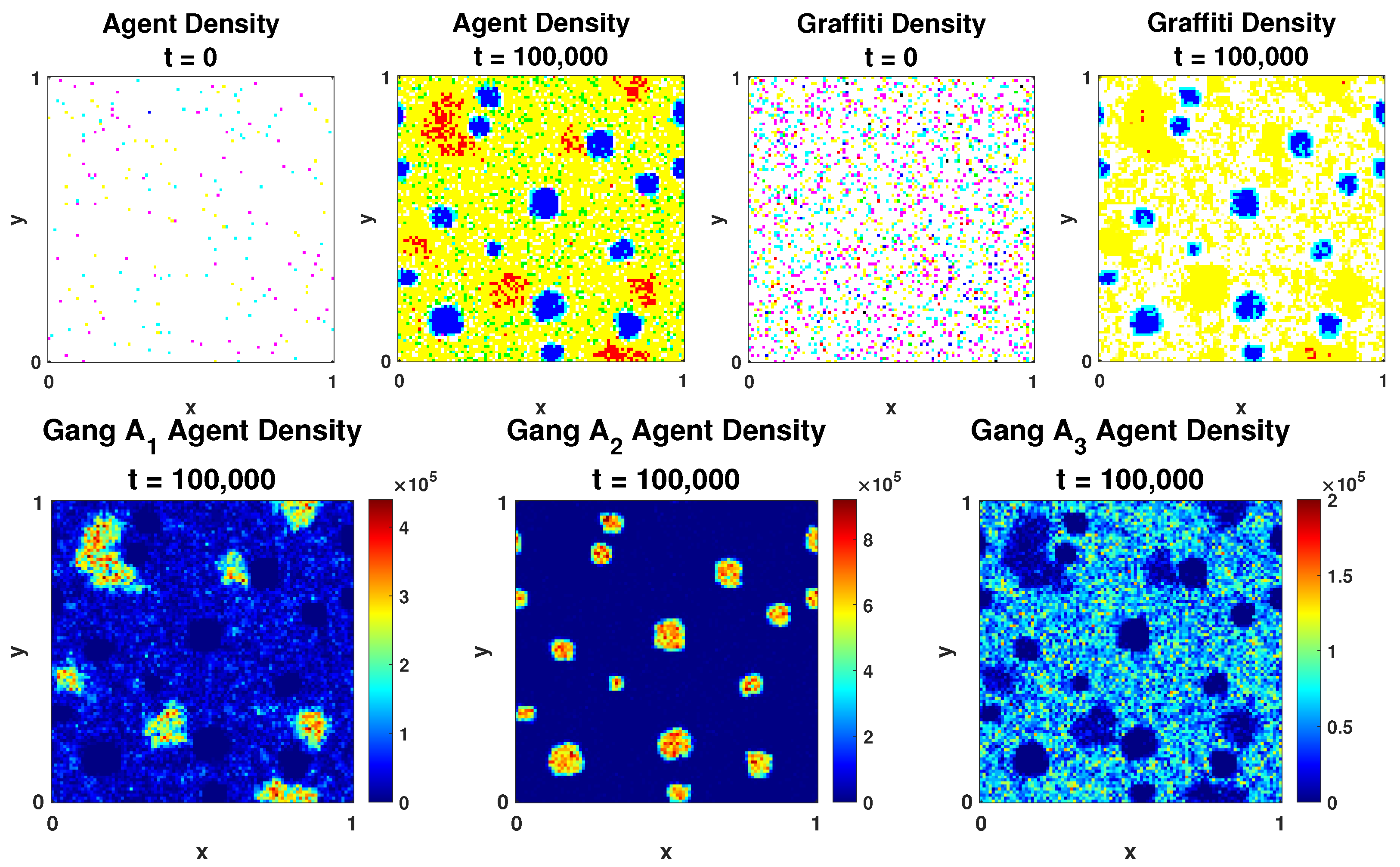
2. Simulations of the Discrete Model

We now will present the results of the simulations of our discrete model. For simplicity, unless otherwise stated, in our simulations we assume we only have $three$ gangs $1,2$ and 3, and that all gangs are assumed to have 50,000 agents. The case $K=3$ will give us insight into the differences between the two-gang model and the multi-gang model that we consider here, while remaining both analytically and visually tractable. We shall also assume that the lattice size $L\times L$ is $100\times 100$ with lattice spacing $l=1/L$, and we will use 100,000 time steps with each step size $\delta t=1$.

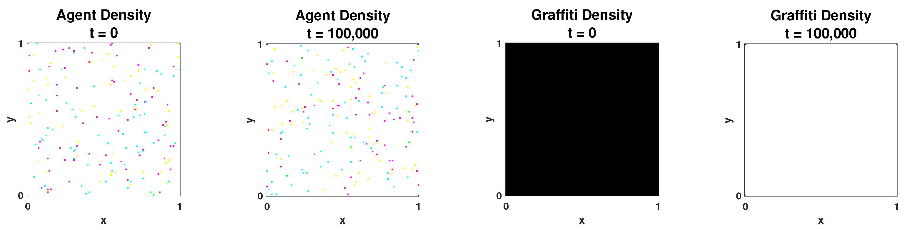
2.1. Well-Mixed State

We start our simulations with $\beta =5\times {10}^{-6}$, and the resulting lattice simulations are visualized in Figure 1. The first two lattices in Figure 1 represent the time evolution of agent density, whereas the last two lattices represent the graffiti density over time. We assign the colors red, blue and green for gangs 1, 2 and 3, respectively. The color white is used if there are the same number of agents or the same amount of graffiti from all gangs at a site. The colors cyan, magenta and yellow are used if a site has two gangs (blue and green, blue and red, or red and green, respectively). Finally, if the site is empty, then it will be assigned the color black.

From Figure 1, we clearly see that the gangs remain well mixed over time for $\beta =5\times {10}^{-6}$. We do not see any patterns being formed for the graffiti, with the initial graffiti lattice black and the final graffiti lattice white, and the gang agents’ movement is in essence a two-dimensional random walk, hardly taking the opposing gangs graffiti into consideration due to the low $\beta$ value. This is due to the way the agents are allowed to move in Equation (3), where a very small $\beta$ values give the agent a probability of nearly $0.25$ to move to each one of the four neighboring sites.

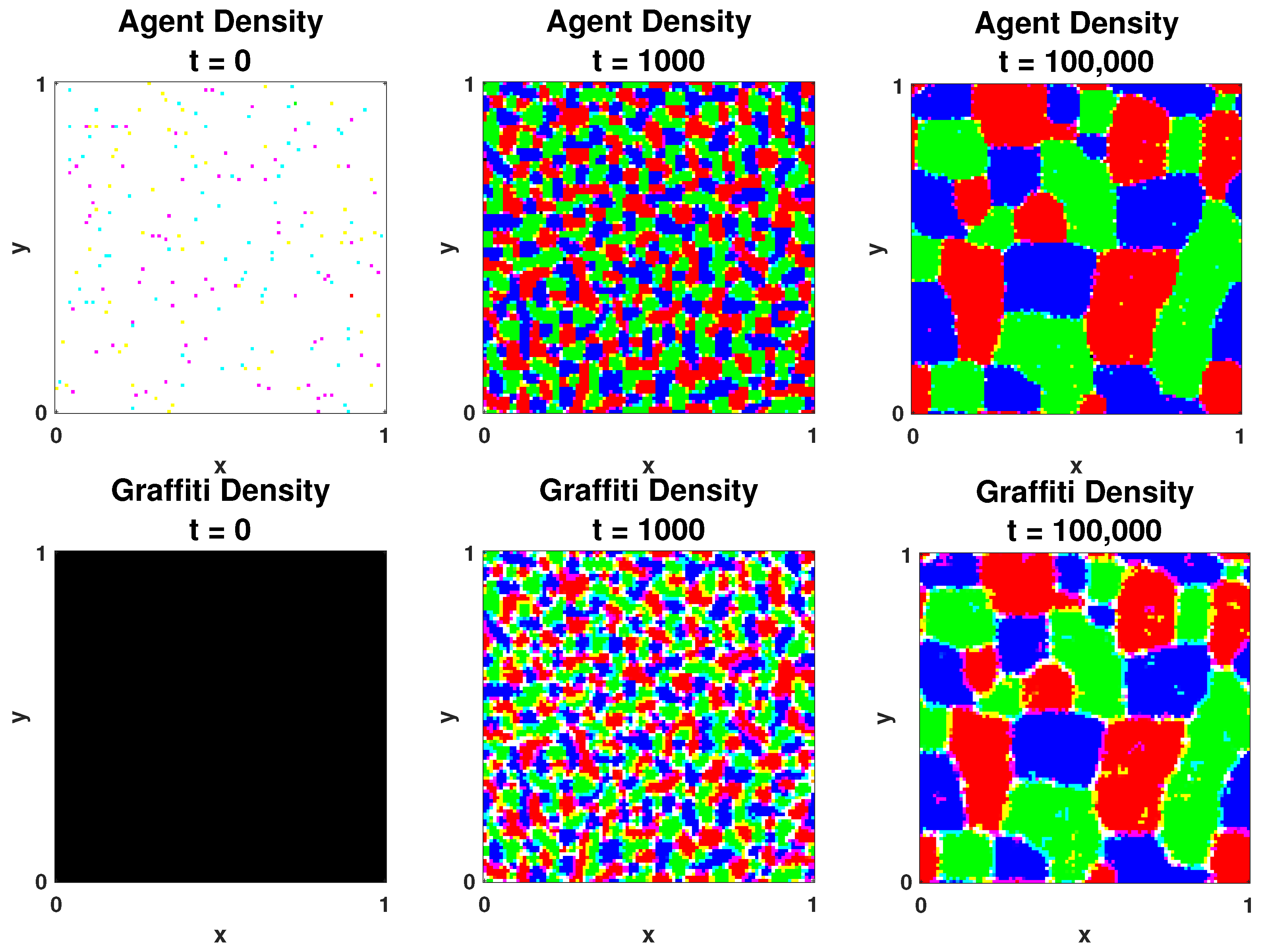
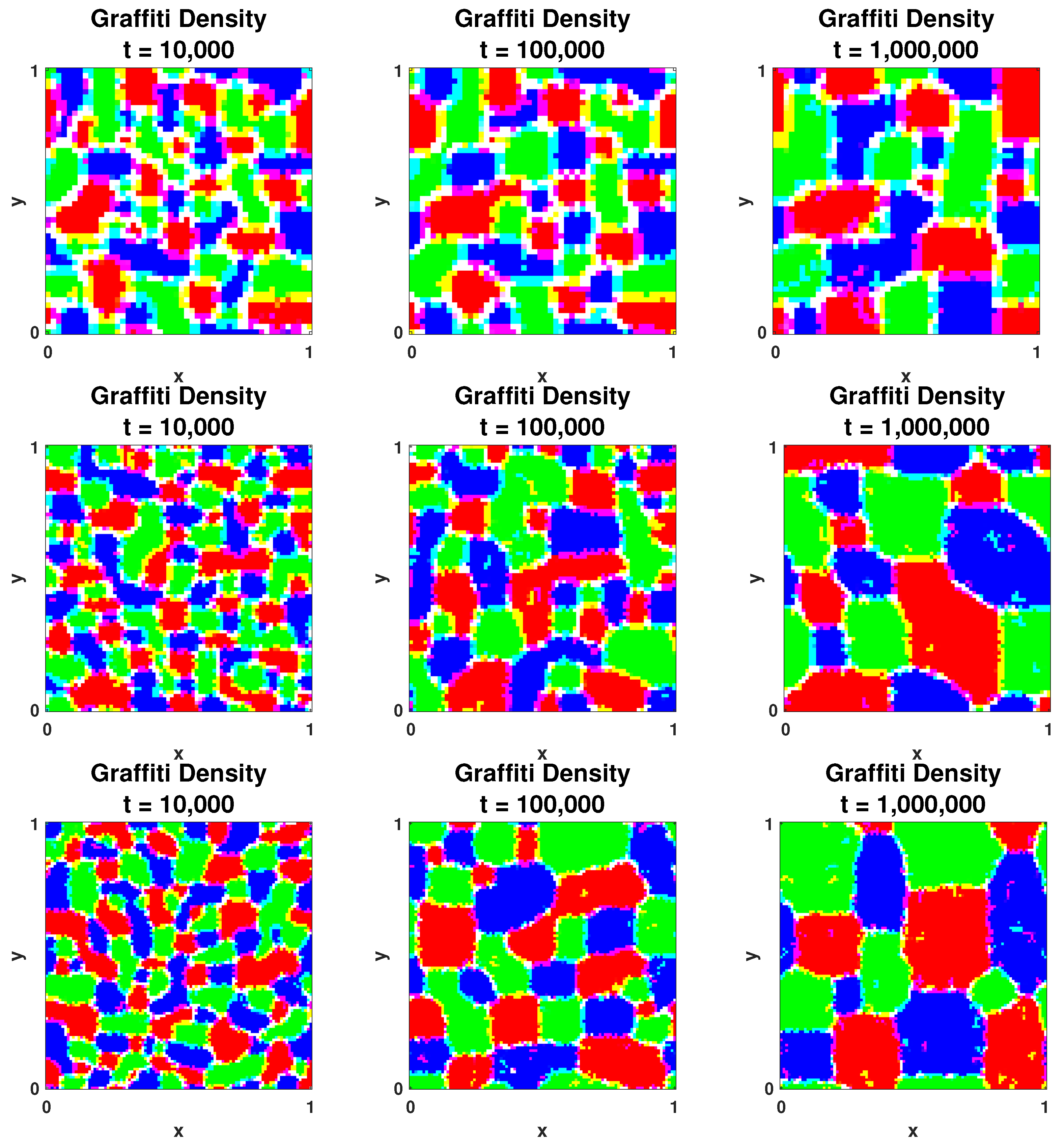
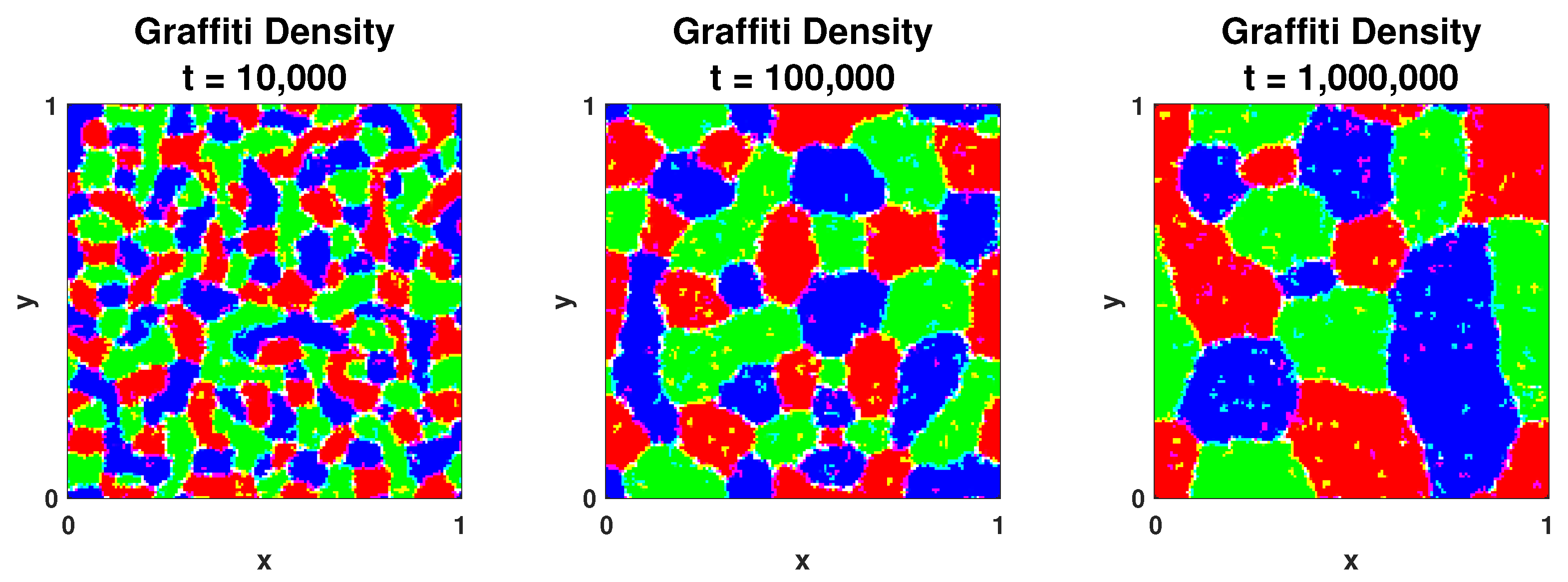
2.2. Segregated State

The value of $\beta$ is now increased so that it is equal to $3\times {10}^{-5}$, and we keep all other parameters the same. The resulting lattice is visualized in Figure 2. The top row illustrates the time evolution of agent density, and the bottom row shows the graffiti density over time.

From Figure 2, we see that initially the agents are well-mixed. However, as time evolves, we see that agents from each gang cluster together to form all-red, all-green and all-blue territories. As time increases, the patterns in both the agent and graffiti densities coarsen. From the same figure, we clearly see that the graffiti density is similar to the agents density and the agents’ movements are based on the other gangs’ graffiti. That is, in this state, the $\beta$ value is large enough that the agents are reacting to the opposing gang graffiti and the agents movement is no longer close to an unbiased random walk. We can also observe from this figure that the areas with more than one gang’s graffiti lie at the boundaries of the territories dominated by each gang. Similarly, this is where we observe the agents overlapping, though to a lesser extent. Presumably, this overlap enables the coarsening seen in the figure. We notice that the segregation seen here in the K group case differs from the patterns seen in the two group model [10]. Here, the territories formed by each of the gangs are convex areas that coalesce over time, remaining convex throughout the territorial evolution. In the two gang model, the patterns are more serpentine and closer to the patterns seen in the Cahn–Hilliard system [35].

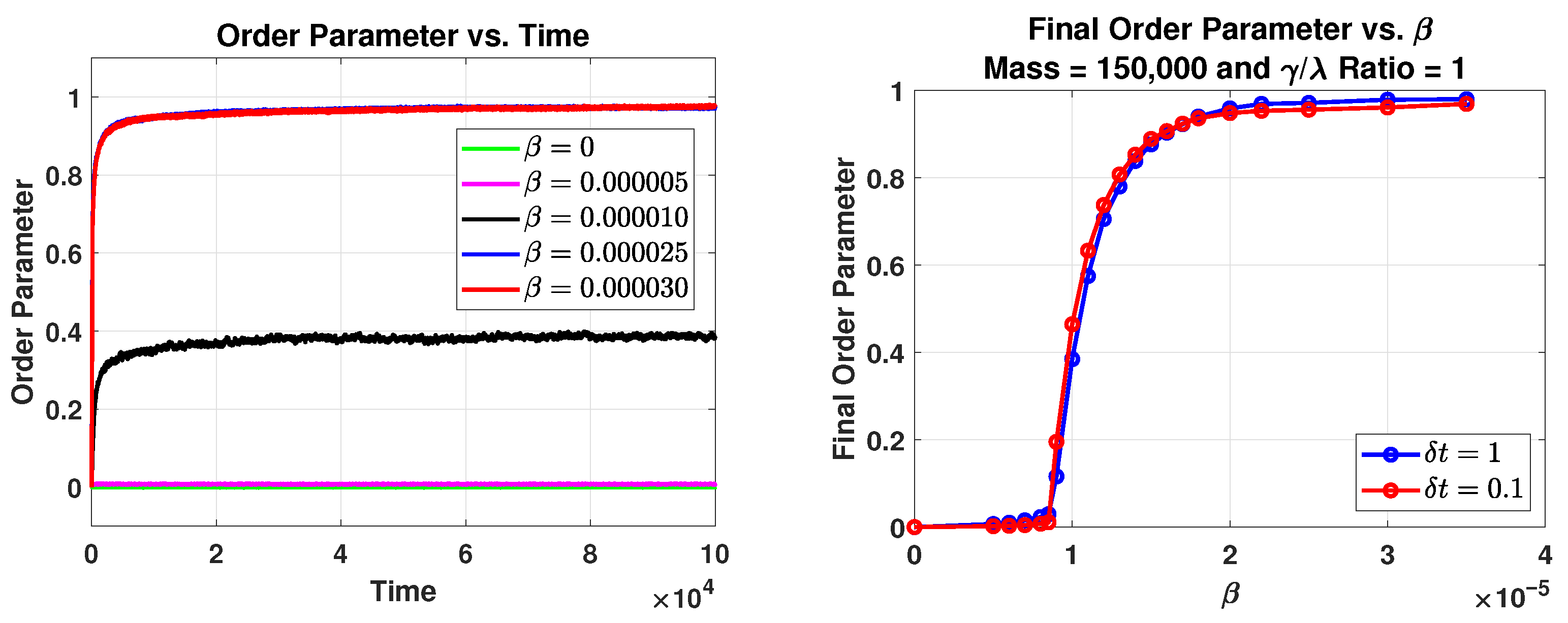
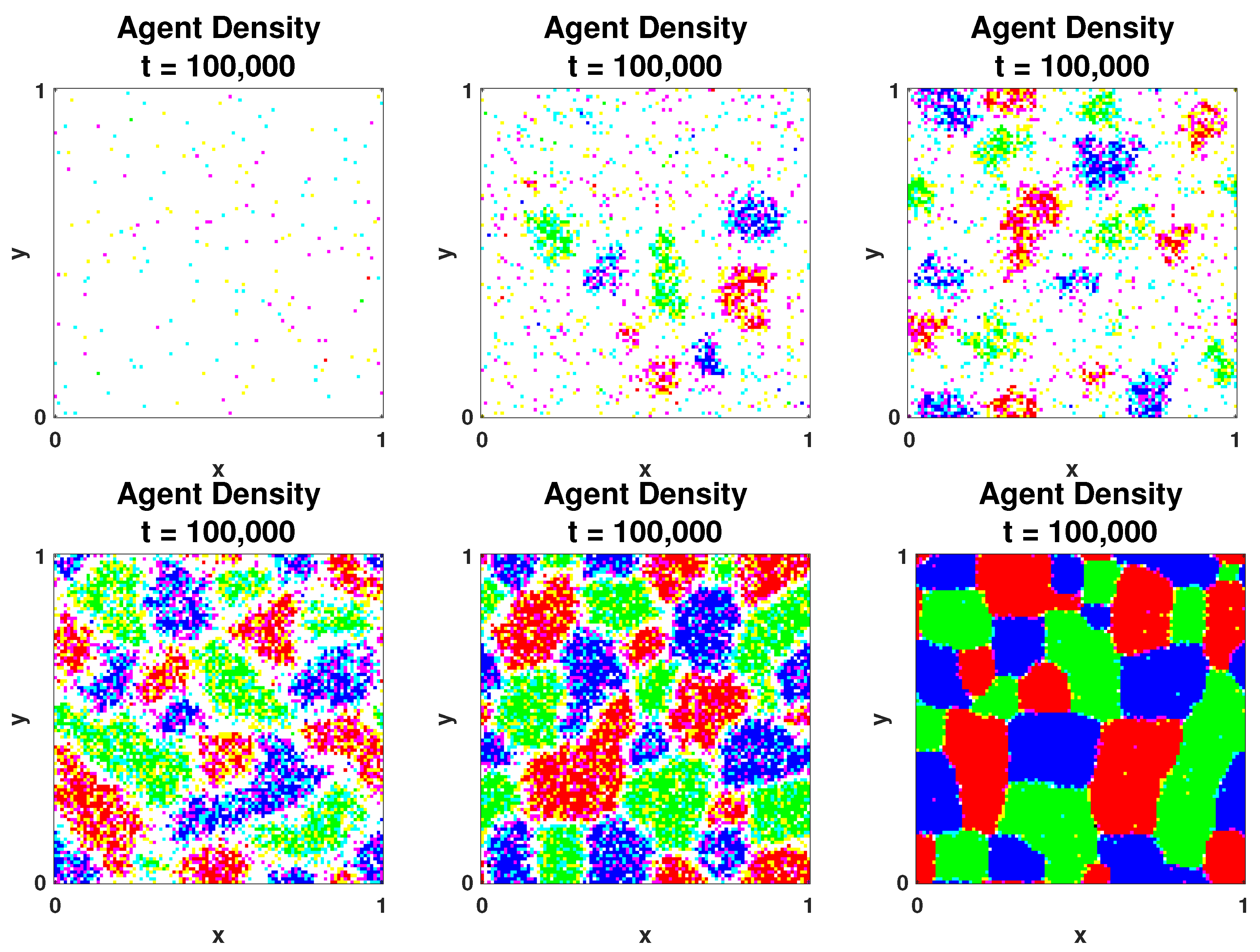
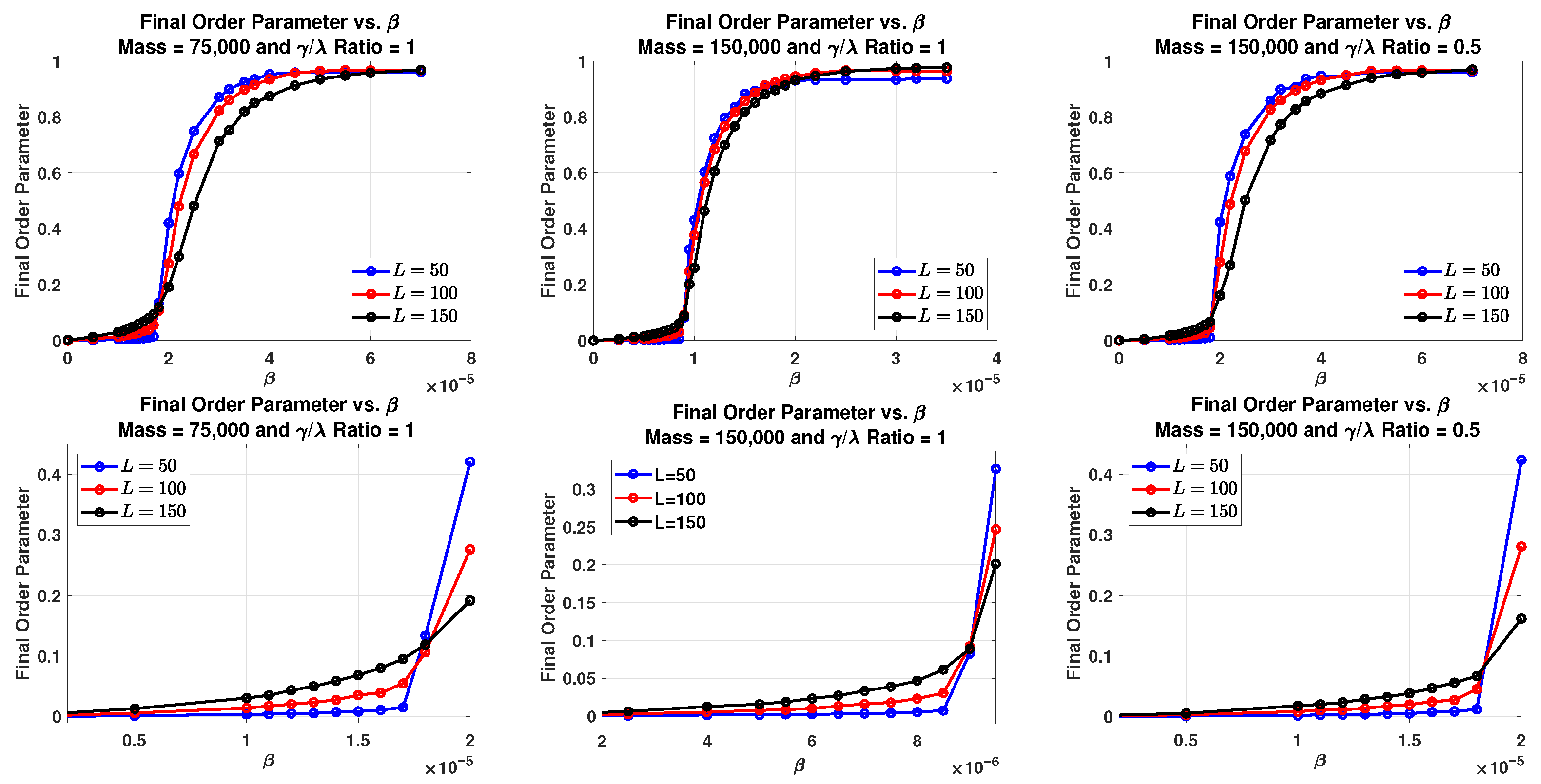
2.3. System Parameters and the Discrete Phase Transition

2.3.1. Effects of $\beta$

In Section 2.1 and Section 2.2, we saw that changing the value of the parameter $\beta$ could lead to a phase transition. In order for us to study the phase transitions, we use the concept of order parameter that we introduced in Section 1.2.2. In Equation (10), we defined an order parameter for a system of three gangs. This order parameter is defined to have a low value for a well-mixed phase and a high value for a segregated phase; in Section 1.2.2, we saw that the order parameter $\mathcal{E}\approx 0$ for a well mixed state and $\mathcal{E}\approx 1$ for a fully segregated state. For our simulations, we graph the order parameter over the course of the simulation for different values of $\beta$, visualizing the output in Figure 3.

We see in the left plot in Figure 3, the time evolution of the order parameter for different $\beta$ values. Here, we easily see that given enough time steps, the order parameter levels off to a certain value, presumably its asymptotic value. We see that for $\beta =0$ and $\beta =0.000005$, the order parameter remained approximately zero throughout all time steps. This is expected, as the system remains well-mixed for these relatively small $\beta$ values. However, we see that once we increase the values of $\beta$, then the order parameter starts to increase. For instance, if $\beta =0.000025$ or $\beta =0.000030$, then the order parameter increases fairly quickly in the first $\mathrm{10,000}$ time steps before leveling off to just under the fully-segregated value of 1 for the remaining time steps. This shows us that for these relatively large $\beta$ values, the system segregates fairly quickly and remains segregated throughout the simulation. Finally, we also see that if we choose $\beta =0.00001$, then the order parameter does increase and the system does exhibit some segregation, but this is not perfect segregation as the order parameter levels off to around $0.4$.

It is evident from the right plot of Figure 3 that there is a critical $\beta$ in which the system undergoes a phase transition. We define the critical $\beta$ to be the value where the order parameter is equal to $0.01$, and denote it by ${\beta }^{*}$. To find the value of ${\beta }^{*}$, we take the final value of the order parameter, which was computed after 100,000 time steps and plot it against different $\beta$ values. The output is then visualized on the right plot of Figure 3. From that plot, we can see that the phase transition occurs when ${\beta }^{*}\in (0.000005,0.000010)$.

To gain better insight into how the system behaves on the steeply rising part of the phase transition curve, we present Figure 4. Here, we can observe how the system looks when it neither well-mixed nor fully segregated, but is instead in a partially segregated state. We visualize in this figure the agent densities after 100,000 time steps for different $\beta$ values. We see that when the order parameter is between $0.1$ and $0.9$, then the system is in a partially segregated state. An interesting observation in Figure 4 is that as $\beta$ increases, the territories emerge from within a well-mixed state and gradually become more defined. However, in many of these partially-segregated states, we see a zone between those territories that is not dominated by any specific gang. We see in the aforementioned figure that this zone gets smaller as $\beta$ increases. In ecological literature, such as the wolf pack model by Lewis et al. [8], it is found that between each neighboring pack, there are buffer zones that are hardly visited by the wolf packs. The buffer zones size changes with time, and the change depends on the different pack scent markings and other different environmental factors such as the climate, and on prey’s existence. This model may be exhibiting a similar phenomenon here.

2.3.2. Effects of Other Parameters

In order to investigate how other parameters such as system mass, time step, lattice size, graffiti rate and decay rate affect the system phase transition, we vary one parameter at a time while keeping all other parameters fixed. This is important, since in the derivation of the continuum equations for our system, we will assume that both the time step $\delta t$ and the lattice spacing l approach zero. It is therefore essential to know if a finer grid affects our discrete model as opposed to a coarser grid. We also would like to know if taking smaller or bigger time steps might affect the rate of segregation and if it has any effect on the phase transition.

We begin by studying how the time step might affect the system. To do that, we keep all our system parameters constant and decrease the time step $\delta t$ from 1 to $0.1$; we then plot the final order parameter value for different $\beta$ values, which were computed after 100,000 time steps. The results are visualized on the right plot in Figure 3. In the plot, it is clear that the smaller time step does not affect the rate of segregation, nor does it affect where the phase transition occurs.

We were also interested in how the mass might affect our system. For our investigation, we compute the final order parameter value after 100,000 time steps. In Figure 5, we see in the first plot that when the mass is 75,000 the critical $\beta$ at which the phase transition occurs is about $1.8\times {10}^{-5}$. However, in the middle plot, the mass is increased to 150,000 and this time the phase transition occurs around $0.9\times {10}^{-5}$. Thus, we notice that as the systems’ mass increases, the resulting phase transition happens at a smaller $\beta$ value. Physically, this makes sense, since having a larger number of agents implies that there will be more graffiti being added at each site and thus a smaller $\beta$ value should be sufficient for the agents to react to the graffiti field.

We also investigated how the ratio $\frac{\gamma }{\lambda }$ might change where the phase transition occurs. Again, we kept all other parameters fixed and changed the value of the ratio by altering the decay rate $\lambda$. Having a higher decay rate means that the graffiti is decaying more quickly and thus each site would have less graffiti. We found that by decreasing the $\frac{\gamma }{\lambda }$ ratio, a higher $\beta$ value is needed for segregation. This is evident in the middle and right plots in Figure 5. There, we clearly see that when the $\frac{\gamma }{\lambda }=1$, the critical $\beta$ is around $0.9\times {10}^{-5}$, whereas when the $\frac{\gamma }{\lambda }$ is decreased to $0.5$, the critical $\beta$ is around $1.8\times {10}^{-5}$. Physically, this is due to the fact that less graffiti on a site means that a larger $\beta$ value is necessary for the agents to react to it.

We are also interested in investigating how changing the grid size affects the segregation when we alter the other parameters. For our investigation, we keep all our parameters constant and vary the grid size by taking $L=50,L=100,$ and $L=150$. After 100,000 time steps, we compute the order parameter for each grid size. The results of all three cases are visualized in Figure 5, where the blue, red, and black curves represent $L=50,L=100,$ and $L=150$, respectively. When comparing the three curves, we see that all curves intersect near the order parameter value of 0.1, which is where we choose the critical $\beta$ value of our system. Although the critical parameter remains the same, making the grid finer leads to the phase transition curve becoming smoother, which is evident in the first and third plots in Figure 5. We see that the process of reaching full segregation becomes more gradual as the grid becomes finer, indicating that our phase transition changes from first-order to second-order as the number of grid points increases.

In Figure 6, we visualize the temporal evolution of the graffiti density for the grid sizes $L=50,L=75,L=100,$ and $L=150$. In all four cases, the graffiti density is similar by time 100,000. However, at time $\mathrm{10,000}$, we see finer structures as L increases and the grid becomes finer. Additionally, we can also see that the boundary region where we observe overlap in the graffiti becomes smaller as L increases, and the territories become smoother and less pixelated.

3. Deriving the Convection-Diffusion System

In this Section, we will formally derive the continuum equations of our system and prove that the limiting system of convection–diffusion equations is

$$\left\{\begin{array}{c}{\displaystyle \frac{\partial {\xi }_j}{\partial t}(x,y,t)=\gamma {\rho }_j(x,y,t)-\lambda {\xi }_j(x,y,t)}\hfill \\ {\displaystyle \frac{\partial {\rho }_j}{\partial t}(x,y,t)=\frac{D}{4}\nabla ·\left[\nabla {\rho }_j(x,y,t)+2\beta \left({\rho }_j(x,y,t)\nabla \left(\sum _{\begin{array}{c}i=1\\ i\ne j\end{array}}^K{\xi }_i(x,y,t)\right)\right)\right]}\hfill \end{array}\right.$$

(13)

on a one-by-one domain with periodic boundary conditions, where $j\in \{1,2,\cdots ,K\}$. Since our discrete model is a multiple-gang extension of the two-species model in [10], we proceed with finding the continuum equations by following the steps of the derivation of the continuum model therein. With minor modifications, the same derivation goes through for this multiple-gang case.

Deriving the continuum limits from discrete models is of great interest to the mathematical community; for example, just from the crime modeling literature, we can refer you to papers [22,26,36,37]. These continuum equations are often formally derived by assuming appropriate smoothness of the gang density and graffiti density and taking both the grid spacing and time step to zero, as we will do here. The continuum partial differential equations give us more tools for understanding the macroscopic behavior of the model.

3.1. Continuum Graffiti Density

We start by formally deriving the continuum equations for graffiti densities, recalling for $j\in \{1,2,\cdots ,K\}$, the discrete model (6):

$${\xi }_j(x,y,t+\delta t)={\xi }_j(x,y,t)-\delta t·\lambda ·{\xi }_j(x,y,t)+\delta t·\gamma ·{\rho }_j(x,y,t).$$

Rearranging the equation and dividing by $\delta t$ gives us:

$$\frac{{\xi }_j(x,y,t+\delta t)-{\xi }_j(x,y,t)}{\delta t}=\gamma ·{\rho }_j(x,y,t)-\lambda ·{\xi }_j(x,y,t).$$

This is now in the form of a difference equation. Assuming sufficient smoothness of the agent and graffiti densities ${\rho }_j$ and ${\xi }_j$, we take $\delta t\to 0$. This gives us the final form of the graffiti continuum equation for gang j:

$$\frac{\partial {\xi }_j}{\partial t}(x,y,t)=\gamma {\rho }_j(x,y,t)-\lambda {\xi }_j(x,y,t).$$

(14)

3.2. Continuum Agent Density

3.2.1. Tools for the Derivation

Deriving the continuum equations for the agent densities is more complex, so before we begin, we define several quantities that will be useful in the derivation. We will need the opposition sum described by Equation (2), which we recall here:

$${\psi }_j(x,y,t):=\sum _{\begin{array}{c}i=1\\ i\ne j\end{array}}^K{\xi }_i(x,y,t).$$

Employing this notation, the first quantity we define is

$$T_j(x,y,t):=\frac{e^{\beta {\psi }_j(x,y,t)}}{4+l^2\left({\beta }^2{\left(\nabla {\psi }_j(x,y,t)\right)}^2-\beta \mathsf{\Delta }{\psi }_j(x,y,t)\right)}.$$

(15)

We will use $T_j$ to account for the influences of the neighbors and neighbor’s neighbors in the discrete model.

Next, we derive approximations to $\nabla T_j$ and $\mathsf{\Delta }{T}_j$, which we will use later in this section. For simplicity, the notation $(x,y,t)$ will be dropped, as there will be no neighbors $(\tilde{x},\tilde{y},t)$ in the derivation of these quantities. We start by simplifying $T_j$ using Taylor series approximations. Applying Taylor expansion to $T_j$ with $x=4$ and $h=l^2\left({\beta }^2{\left(\nabla {\psi }_j\right)}^2-\beta \mathsf{\Delta }{\psi }_j\right)$:

$$\begin{array}{cc}\hfill T_j& =\frac{e^{\beta {\psi }_j}}{4}\left(1-\frac{l^2}{4}\left({\beta }^2{\left(\nabla {\psi }_j\right)}^2-\beta \mathsf{\Delta }{\psi }_j\right)\right)+\mathcal{O}\left(l^4\right).\hfill \end{array}$$

(16)

Note that here, we are depending on the smoothness of ${\psi }_j$. Then, by taking the gradient of (16), we find that

$$\begin{array}{cc}\hfill \nabla T_j& =\frac{e^{\beta {\psi }_j}}{4}\left(\beta \nabla {\psi }_j-\frac{l^2}{4}\left({\beta }^3{(\nabla {\psi }_j)}^3+{\beta }^2\nabla {\psi }_j\mathsf{\Delta }{\psi }_j-\beta {\nabla }^3{\psi }_j\right)\right)+\mathcal{O}\left(l^4\right).\hfill \end{array}$$

(17)

We also can find $\mathsf{\Delta }{T}_j$:

$$\begin{array}{cc}\hfill \mathsf{\Delta }{T}_j& =\frac{e^{\beta {\psi }_j}}{4}(\left({\beta }^2{(\nabla {\psi }_j)}^2+\beta \mathsf{\Delta }{\psi }_j\right)-\frac{l^2}{4}(4{\beta }^3{(\nabla {\psi }_j)}^2\mathsf{\Delta }{\psi }_j\hfill \\ \hfill & +{\beta }^2{\left(\mathsf{\Delta }{\psi }_j\right)}^2+{\beta }^4{(\nabla {\psi }_j)}^4-\beta {\nabla }^4{\psi }_j\left)\right)+\mathcal{O}\left(l^4\right).\hfill \end{array}$$

(18)

Modifying definition (3) so that we evaluate the probability that an agent at a neighboring site $(\tilde{x},\tilde{y})$ moves to site $(x,y)$:

$$M_j(\tilde{x}\to x,\tilde{y}\to y,t)=\frac{e^{-\beta {\psi }_j(x,y,t)}}{{\displaystyle \sum _{(\tilde{\tilde{x}},\tilde{\tilde{y}})\sim (\tilde{x},\tilde{y})}}{e}^{-\beta {\psi }_j(\tilde{\tilde{x}},\tilde{\tilde{y}},t)}},$$

(19)

where $(\tilde{\tilde{x}},\tilde{\tilde{y}})$ are the four neighbors of site $(\tilde{x},\tilde{y})$. To remove the presence of the neighbors’ neighbors $(\tilde{\tilde{x}},\tilde{\tilde{y}})$ from the denominator, we apply the discrete Laplacian to find that

$$\sum _{(\tilde{\tilde{x}},\tilde{\tilde{y}})\sim (\tilde{x},\tilde{y})}{e}^{-\beta {\psi }_j(\tilde{\tilde{x}},\tilde{\tilde{y}},t)}=4e^{-\beta {\psi }_j(\tilde{x},\tilde{y},t)}+l^2\mathsf{\Delta }\left(e^{-\beta {\psi }_j(\tilde{x},\tilde{y},t)}\right)+\mathcal{O}\left(l^4\right).$$

(20)

Noting that

$$\mathsf{\Delta }{e}^{-\beta {\psi }_j(\tilde{x},\tilde{y},t)}=\left[{\beta }^2{\left(\nabla {\psi }_j(\tilde{x},\tilde{y},t)\right)}^2-\beta \mathsf{\Delta }{\psi }_j(\tilde{x},\tilde{y},t)\right]e^{-\beta {\psi }_j(\tilde{x},\tilde{y},t)}.$$

(21)

Combining Equations (20) and (21) gives us

$$\begin{array}{cc}\hfill \sum _{(\tilde{\tilde{x}},\tilde{\tilde{y}})\sim (\tilde{x},\tilde{y})}{e}^{-\beta {\psi }_j(\tilde{\tilde{x}},\tilde{\tilde{y}},t)}=& e^{-\beta {\psi }_j(\tilde{x},\tilde{y},t)}\left(4+l^2\left({\beta }^2{\left(\nabla {\psi }_j(\tilde{x},\tilde{y},t)\right)}^2-\beta \mathsf{\Delta }{\psi }_j(\tilde{x},\tilde{y},t)\right)\right)\hfill \\ \hfill & +\mathcal{O}\left(l^4\right).\hfill \end{array}$$

Substituting it back into Equation (19), and replacing the denominator gives us

$$\begin{array}{cc}\hfill M_j(\tilde{x}\to x,\tilde{y}\to y,t)& =\frac{e^{-\beta {\psi }_j(x,y,t)}}{\left[4+l^2\left({\beta }^2{\left(\nabla {\psi }_j(\tilde{x},\tilde{y},t)\right)}^2-\beta \mathsf{\Delta }{\psi }_j(\tilde{x},\tilde{y},t)\right)\right]e^{-\beta {\psi }_j(\tilde{x},\tilde{y},t)}+\mathcal{O}\left(l^4\right)}\hfill \\ \hfill & \approx e^{-\beta {\psi }_j(x,y,t)}\left[\frac{e^{\beta {\psi }_j(\tilde{x},\tilde{y},t)}}{4+l^2\left({\beta }^2{\left(\nabla {\psi }_j(\tilde{x},\tilde{y},t)\right)}^2-\beta \mathsf{\Delta }{\psi }_j(\tilde{x},\tilde{y},t)\right)}\right].\hfill \end{array}$$

The term inside the large brackets in the equation above takes the form of (15) where $(x,y,t)$ is replaced with $(\tilde{x},\tilde{y},t)$, yielding the following approximation:

$$M_j(\tilde{x}\to x,\tilde{y}\to y,t)\approx e^{-\beta {\psi }_j(x,y,t)}{T}_j(\tilde{x},\tilde{y},t).$$

(22)

3.2.2. The Derivation

We now have all the tools needed to formally derive the agent density continuum equations. We will be using the discrete Laplacian approximation in order to approximate the influence of the neighbors of site $(x,y)$. We will also be using Equation (22) to simplify the discrete model.

Starting from the discrete model, we recall Equation (5):

$$\begin{array}{cc}\hfill {\rho }_j(x,y,t+\delta t)=& {\rho }_j(x,y,t)+\sum _{(\tilde{x},\tilde{y})\sim (x,y)}{\rho }_j(\tilde{x},\tilde{y},t)M_j(\tilde{x}\to x,\tilde{y}\to y,t)\hfill \\ \hfill & -{\rho }_j(x,y,t)\sum _{(\tilde{x},\tilde{y})\sim (x,y)}{M}_j(x\to \tilde{x},y\to \tilde{y},t).\hfill \end{array}$$

Rearranging the equation and dividing both sides by $\delta t$ gives us

$$\begin{array}{c}\hfill \frac{{\rho }_j(x,y,t+\delta t)-{\rho }_j(x,y,t)}{\delta t}=\frac{1}{\delta t}\left[\sum _{(\tilde{x},\tilde{y})\sim (x,y)}{\rho }_j(\tilde{x},\tilde{y},t)M_j(\tilde{x}\to x,\tilde{y}\to y,t)\right.\\ \hfill \left.-{\rho }_j(x,y,t)\sum _{(\tilde{x},\tilde{y})\sim (x,y)}{M}_j(x\to \tilde{x},y\to \tilde{y},t)\right].\end{array}$$

By Equation (22), and noting that each agent has to move to one of the neighboring sites,

$$\begin{array}{cc}\hfill \frac{{\rho }_j(x,y,t+\delta t)-{\rho }_j(x,y,t)}{\delta t}=\frac{1}{\delta t}[& e^{-\beta {\psi }_j(x,y,t)}\sum _{(\tilde{x},\tilde{y})\sim (x,y)}{\rho }_j(\tilde{x},\tilde{y},t)T_j(\tilde{x},\tilde{y},t)\hfill \\ \hfill -& {\rho }_j(x,y,t)+\mathcal{O}\left(l^4\right)].\hfill \end{array}$$

(23)

The notation $(x,y,t)$ is again dropped as there are no longer any neighbors $(\tilde{x},\tilde{y},t)$ remaining in this derivation. Now, using the discrete Laplacian technique, we can approximate the contribution of the neighboring sites, giving on the right-hand side

$$\frac{1}{\delta t}\left[e^{-\beta {\psi }_j}\left(4{\rho }_j{T}_j+l^2\mathsf{\Delta }\left({\rho }_j{T}_j)\right)\right)-{\rho }_j+\mathcal{O}\left(l^4\right)\right].$$

(24)

From definition (15), $T_j(x,y,t)$ is substituted back into the first term of (24), and further simplifying yields:

$$\frac{1}{\delta t}\left[4{\rho }_j\left(\frac{1}{4+l^2\left({\left(\beta \nabla {\psi }_j\right)}^2-\beta \mathsf{\Delta }{\psi }_j\right)}\right)-{\rho }_j+l^2{e}^{-\beta {\psi }_j}\mathsf{\Delta }\left({\rho }_j{T}_j\right)+\mathcal{O}\left(l^4\right)\right].$$

(25)

Using a Taylor series expansion on the first term within the brackets yields,

$$\left(\frac{1}{4+l^2\left({\left(\beta \nabla {\psi }_j\right)}^2-\beta \mathsf{\Delta }{\psi }_j\right)}\right)=\frac{1}{4}-\frac{l^2\left({\left(\beta \nabla {\psi }_j\right)}^2-\beta \mathsf{\Delta }{\psi }_j\right)}{4^2}+\mathcal{O}\left(l^4\right).$$

Expression (25) thus becomes,

$$\frac{1}{\delta t}\left[4{\rho }_j\left(\frac{1}{4}-\frac{l^2\left({\left(\beta \nabla {\psi }_j\right)}^2-\beta \mathsf{\Delta }{\psi }_j\right)}{4^2}\right)-{\rho }_j+l^2{e}^{-\beta {\psi }_j}\mathsf{\Delta }\left({\rho }_j{T}_j\right)+\mathcal{O}\left(l^4\right)\right].$$

Simplifying the expression yields

$$\begin{array}{cc}\hfill \frac{{\rho }_j(x,y,t+\delta t)-{\rho }_j(x,y,t)}{\delta t}=& \frac{l^2}{\delta t}\left[-\frac{{\rho }_j}{4}\left({\left(\beta \nabla {\psi }_j\right)}^2-\beta \mathsf{\Delta }{\psi }_j\right)+e^{-\beta {\psi }_j}\mathsf{\Delta }\left({\rho }_j{T}_j\right)\right]\hfill \\ \hfill & +\mathcal{O}\left(\frac{l^4}{\delta t}\right).\hfill \end{array}$$

(26)

However, we can further simplify this by noting that

$$\mathsf{\Delta }\left({\rho }_j{T}_j\right)=\left(T_j\mathsf{\Delta }{\rho }_j+2\nabla T_j\nabla {\rho }_j+{\rho }_j\mathsf{\Delta }{T}_j\right).$$

From (16) through (18), we have

$$\begin{array}{cc}\hfill T_j& =\frac{e^{\beta {\psi }_j}}{4}+\mathcal{O}\left(l^2\right),\hfill \\ \hfill \nabla T_j& =\frac{\beta e^{\beta {\psi }_j}}{4}\nabla {\psi }_j+\mathcal{O}\left(l^2\right),\hfill \\ \hfill \mathsf{\Delta }{T}_j& =\frac{e^{\beta {\psi }_j}}{4}\left(\beta \mathsf{\Delta }{\psi }_j+{(\beta \nabla {\psi }_j)}^2\right)+\mathcal{O}\left(l^2\right).\hfill \end{array}$$

Therefore,

$$\begin{array}{cc}\hfill \mathsf{\Delta }\left({\rho }_j{T}_j\right)& =\frac{e^{\beta {\psi }_j}}{4}\mathsf{\Delta }{\rho }_j+\frac{2\beta e^{\beta {\psi }_j}}{4}\nabla {\psi }_j\nabla {\rho }_j+\frac{e^{\beta {\psi }_j}}{4}{\rho }_j\left(\beta \mathsf{\Delta }{\psi }_j+{(\beta \nabla {\psi }_j)}^2\right)+\mathcal{O}\left(l^2\right)\hfill \\ \hfill & =\frac{e^{\beta {\psi }_j}}{4}\left[\mathsf{\Delta }{\rho }_j+2\beta \nabla {\psi }_j\nabla {\rho }_j+{\rho }_j\left({\left(\beta \nabla {\psi }_j\right)}^2+\beta \mathsf{\Delta }{\psi }_j\right)\right]+\mathcal{O}\left(l^2\right).\hfill \end{array}$$

(27)

Substituting (27) back into (26) gives us

$$\begin{array}{cc}\hfill \frac{{\rho }_j(x,y,t+\delta t)-{\rho }_j(x,y,t)}{\delta t}& =\frac{l^2}{4\delta t}[-{\rho }_j\left({(\beta \nabla {\psi }_j)}^2-\beta \mathsf{\Delta }{\psi }_j\right)+\mathsf{\Delta }{\rho }_j+2\beta \nabla {\psi }_j\nabla {\rho }_j\hfill \\ \hfill & +{\rho }_j\left({\left(\beta \nabla {\psi }_j\right)}^2+\beta \mathsf{\Delta }{\psi }_j\right)]+\mathcal{O}\left(\frac{l^4}{\delta t}\right)\hfill \\ \hfill & =\frac{l^2}{4\delta t}\nabla ·\left[\nabla {\rho }_j+2\beta \left({\rho }_j\nabla {\psi }_j\right)\right]+\mathcal{O}\left(\frac{l^4}{\delta t}\right).\hfill \end{array}$$

Assuming that the agent density ${\rho }_j$ is sufficiently smooth and the following limits

$$\begin{array}{cc}\hfill l& \to 0,\hfill \\ \hfill \delta t& \to 0,\hfill \\ \hfill \frac{l^2}{\delta t}& \to D,\hfill \end{array}$$

(28)

gives us the final form for the continuum equations for the density of gang j agents:

$$\frac{\partial {\rho }_j}{\partial t}=\frac{D}{4}\nabla ·\left[\nabla {\rho }_j+2\beta \left({\rho }_j\nabla {\psi }_j\right)\right].$$

(29)

Finally, from (14) and (29), and using Equation (2) to express everything in terms of agent density and graffiti density, the limiting convection–diffusion system for our model is

$$\left\{\begin{array}{c}{\displaystyle \frac{\partial {\xi }_j}{\partial t}(x,y,t)=\gamma {\rho }_j(x,y,t)-\lambda {\xi }_j(x,y,t)}\hfill \\ {\displaystyle \frac{\partial {\rho }_j}{\partial t}(x,y,t)=\frac{D}{4}\nabla ·\left[\nabla {\rho }_j(x,y,t)+2\beta \left({\rho }_j(x,y,t)\nabla \left(\sum _{\begin{array}{c}i=1\\ i\ne j\end{array}}^K{\xi }_i(x,y,t)\right)\right)\right]}\hfill \end{array}\right.$$

(30)

for $j=1,2,\cdots ,K$ on a one-by-one domain with periodic boundary conditions.

Upon examination of (30), we can see that each group’s graffiti evolution is entirely dependent on the group’s own agent and graffiti densities at that location. The agent density at that point contributes to the growth of the graffiti density, and the graffiti decays proportionally to its current density. This is exactly what we would expect from the discrete model. An important feature that distinguishes this model from other chemo-attractant or chemo-repellent systems is that there is no diffusion of the graffiti.

The evolution equations for the agent densities are more complex. However, the evolution equation takes the form of a conservation equation, so we can clearly see that the mass of each group’s agents is conserved. We also observe that the equations retain the features that we expect from the discrete model: the group’s agent density diffuses, in accordance with the random walk in the discrete model, and this diffusion is the main driver of the evolution when parameter $\beta$ is close to zero. Additionally, we observe that the coupling between different groups in the continuum system occurs entirely through the term, which is multiplied by $\beta$. This term drives the density of the group’s agents down the gradient of the sum of the other gangs’ graffiti. When $\beta$ grows larger, this dominates the evolution for the agent densities.

The system of convection–diffusion equations also allow us to clearly see how the parameters affect the behavior of the system. First of all, if $\gamma =0$, no graffiti is ever present, hence $\beta$ and $\lambda$ never come into play, and the agent densities are purely diffusive. If $\gamma \ne 0$, then large $\lambda$ drives down the amount of graffiti, and $\beta$ must be similarly larger to maintain its relevance in the agent density equation. As noted above, we can see that small $\beta$ allows diffusion to dominate, while large $\beta$ forces the agents away from areas with lots of graffiti from the other groups. This agrees with the behavior of the discrete system that we can observe in Figure 4. Finally, the new parameter introduced by this derivation, D, which corresponds to the ratio of the square lattice spacing to the time step, affects the speed of the evolution of the group density. Having this continuum system gives us more tools to examine the impact of the various parameters, which we shall do in Section 4.

3.3. Steady-State Solutions

Considering steady-state solutions for the graffiti density, we find from the evolution equations for the graffiti density that

$$\begin{array}{cc}\hfill \frac{\partial {\xi }_j}{\partial t}(x,y,t)& =0\hfill \\ \hfill \Rightarrow \gamma {\rho }_j(x,y,t)-\lambda {\xi }_j(x,y,t)& =0\hfill \\ \hfill \Rightarrow {\xi }_j& =\frac{\gamma }{\lambda }{\rho }_j.\hfill \end{array}$$

(31)

We now focus our attention on the steady-state solutions for the agent density of gang j:

$$\begin{array}{cc}\hfill \frac{\partial {\rho }_j}{\partial t}(x,y,t)=\frac{D}{4}\nabla ·\left[\nabla {\rho }_j(x,y,t)+2\beta \left({\rho }_j(x,y,t)\nabla \left(\sum _{\begin{array}{c}i=1\\ i\ne j\end{array}}^K{\xi }_i(x,y,t)\right)\right)\right]& =0,\hfill \end{array}$$

considering solutions of the form

$$\begin{array}{cc}\hfill \nabla {\rho }_j(x,y,t)+2\beta \left({\rho }_j(x,y,t)\nabla \left(\sum _{\begin{array}{c}i=1\\ i\ne j\end{array}}^K{\xi }_i(x,y,t)\right)\right)& =k_j,\hfill \end{array}$$

for some constant $k_j\in \mathbb{R}$. Using the steady-state graffiti density derived in Equation (31), we find that

$$\begin{array}{cc}\hfill \nabla {\rho }_j(x,y,t)& =-\frac{2\beta {\gamma }^2}{{\lambda }^2}\left({\rho }_j(x,y,t)\nabla \left(\sum _{\begin{array}{c}i=1\\ i\ne j\end{array}}^K{\rho }_i(x,y,t)\right)\right)+k_j.\hfill \end{array}$$

(32)

Any form of ${\rho }_j(x,y,t)$ satisfying the above equation is a steady-state solution of our system. We observe that the steady-states are those where the gradients of the population j and the opposition graffiti are inversely related. This explains our numerical observations in the discrete model. In the discrete model, the solutions seem to prefer states where the agent densities are nearly constant inside their domain, but have a steep negative gradient at the boundary, where there is a correspondingly steep positive gradient in the sum of the other gangs’ graffiti. This can be seen, for example, in Figure 2.

For simplicity, in the next Section, we consider the steady-states where ${\rho }_j$ is a constant for all j. These clearly satisfy (32). In this case, the steady-state solution of our problem takes the form:

$$\begin{array}{c}\hfill \left\{\begin{array}{cc}{\xi }_j\hfill & =\frac{\gamma }{\lambda }{\rho }_j,\hfill \\ {\rho }_j\hfill & =c_j,\hfill \end{array}\right.\end{array}$$

(33)

for $j=1,2,\cdots ,K$, with $c_j$ a positive constant.

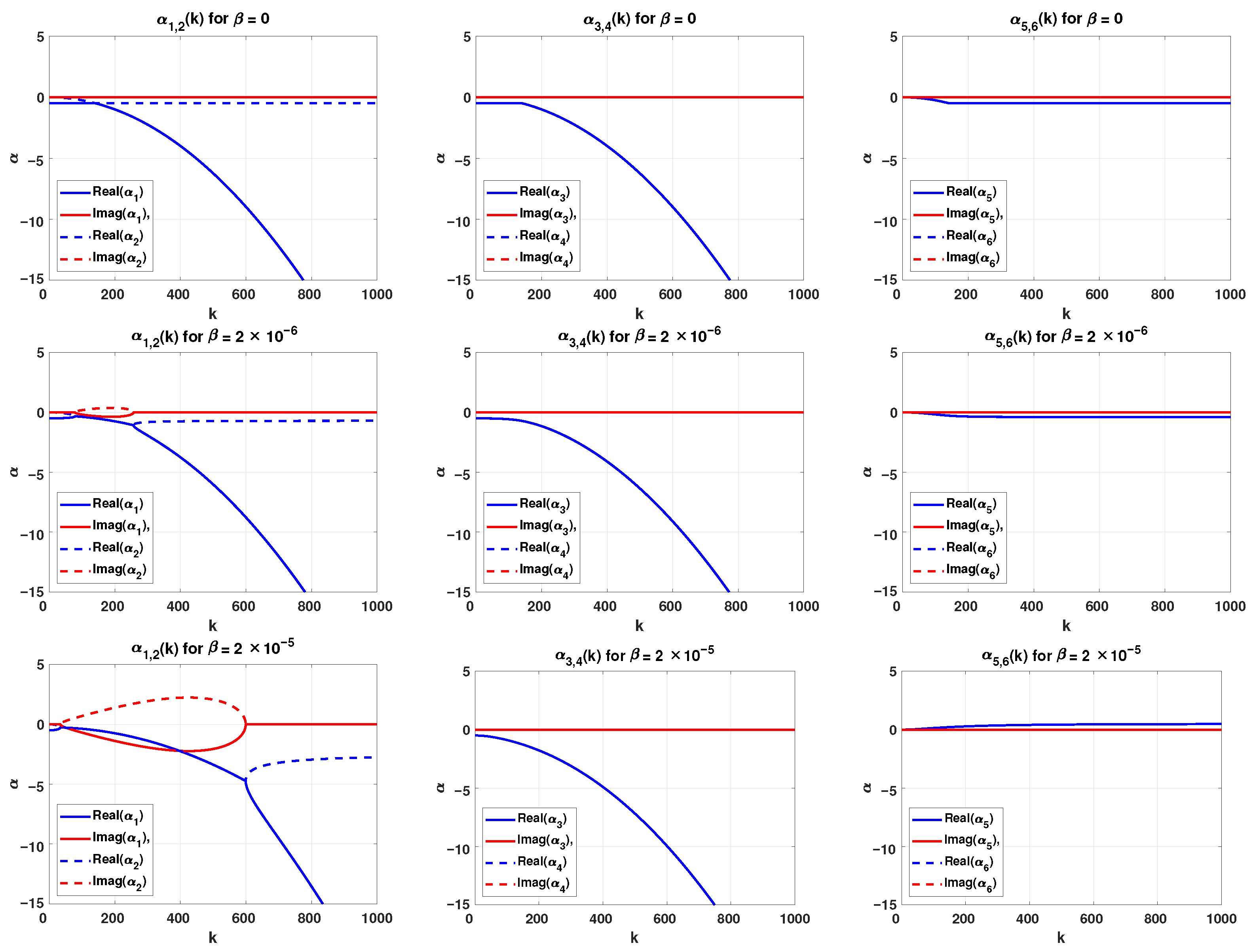
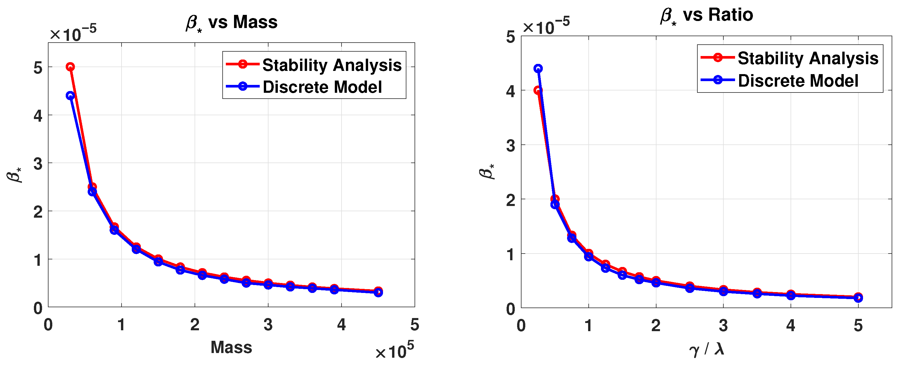
4. Linear Stability Analysis

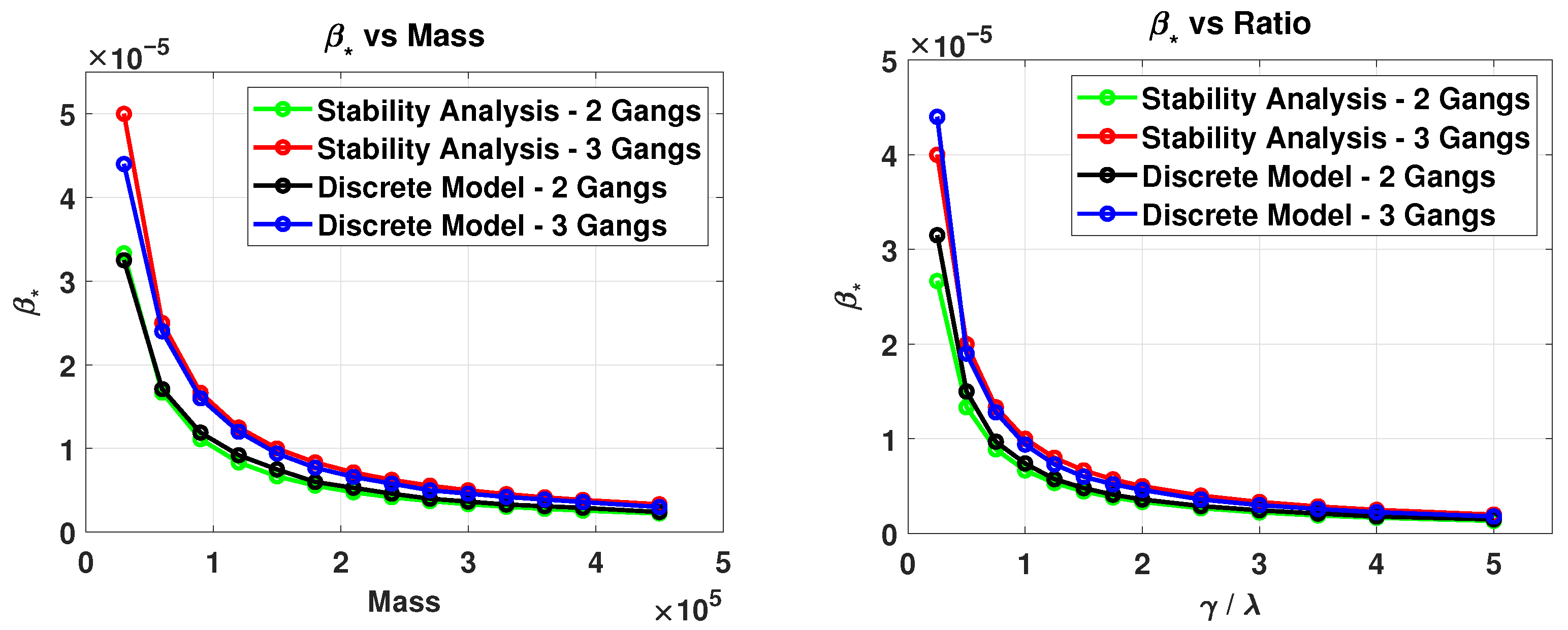
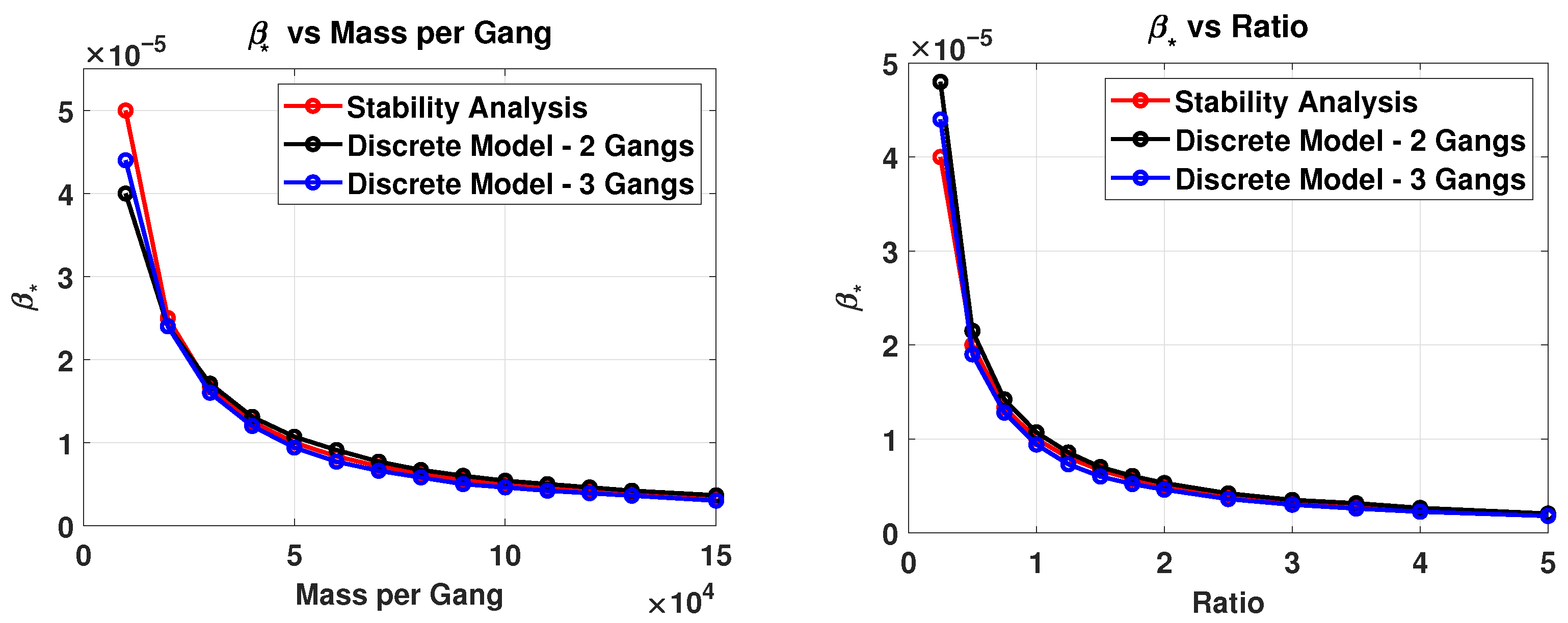
To have a better understanding of the connection between the discrete model and the system of PDEs that we have found, we linearize our model and consider a perturbation of the equilibrium solution (33) to the well-mixed state. We assume that our perturbations are of the form $ϵ=\delta e^{\alpha t}{e}^{i\mathbf{k}·\mathbf{x}}$, with small parameter $\delta <<1$ and $\mathbf{k}$ and $\mathbf{x}$ in ${\mathbb{R}}^2$. In this case, our solution takes the following form:

$$\begin{array}{c}\hfill \left\{\begin{array}{cc}{\xi }_j\hfill & =\overline{{\xi }_j}+{\delta }_{{\xi }_j}{e}^{\alpha t}{e}^{i\mathbf{k}·\mathbf{x}},\hfill \\ {\rho }_j\hfill & =\overline{{\rho }_j}+{\delta }_{{\rho }_j}{e}^{\alpha t}{e}^{i\mathbf{k}·\mathbf{x}}.\hfill \end{array}\right.\end{array}$$

(34)

Here, $e^{i\mathbf{k}·\mathbf{x}}=cos(\mathbf{k}·\mathbf{x})+isin(\mathbf{k}·\mathbf{x})$, where $\mathbf{k}$ represents the wave numbers of the spatial waves in the horizontal and vertical directions. In order for the equilibrium solution to be stable, $\alpha$ must be negative so that it forces the perturbations to decay as time increases. For more examples of this kind of perturbation being used to study the stability of equilibrium solutions, the interested reader is referred to [22,26,38,39].

To analyze the dynamics of these solutions, we now substitute (34) into the evolution Equation (30). We start with the first equation:

$$\frac{\partial {\xi }_j}{\partial t}=\gamma {\rho }_j-\lambda {\xi }_j.$$

(35)

Substituting (34) into (35) yields

$$\begin{array}{cc}\hfill \frac{\partial }{\partial t}\left(\overline{{\xi }_j}+{\delta }_{{\xi }_j}{e}^{\alpha t}{e}^{i\mathbf{k}·\mathbf{x}}\right)& =\gamma (\overline{{\rho }_j}+{\delta }_{{\rho }_j}{e}^{\alpha t}{e}^{i\mathbf{k}·\mathbf{x}})-\lambda (\overline{{\xi }_j}+{\delta }_{{\xi }_j}{e}^{\alpha t}{e}^{i\mathbf{k}·\mathbf{x}}).\hfill \end{array}$$

Since we assumed $\overline{{\xi }_j}$ to be an equilibrium solution, its derivative with respect to time is zero, leading to

$$\begin{array}{cc}\hfill \alpha {\delta }_{{\xi }_j}{e}^{\alpha t}{e}^{i\mathbf{k}·\mathbf{x}}& =(\gamma \overline{{\rho }_j}-\lambda \overline{{\xi }_j})+(\gamma {\delta }_{{\rho }_j}-\lambda {\delta }_{{\xi }_j})e^{\alpha t}{e}^{i\mathbf{k}·\mathbf{x}},\hfill \\ \hfill & =(\gamma {\delta }_{{\rho }_j}-\lambda {\delta }_{{\xi }_j})e^{\alpha t}{e}^{i\mathbf{k}·\mathbf{x}},\hfill \end{array}$$

since $\gamma \overline{{\rho }_j}-\lambda \overline{{\xi }_j}=\frac{\partial \overline{{\xi }_j}}{\partial t}=0$. Hence,

$$\begin{array}{cc}\hfill \alpha {\delta }_{{\xi }_j}& =(\gamma {\delta }_{{\rho }_j}-\lambda {\delta }_{{\xi }_j}),\mathrm{for}j=1,2,\dots ,K\hfill \end{array}$$

(36)

Next, we substitute (34) into the evolution equation for the agent density

$$\frac{\partial {\rho }_j}{\partial t}=\frac{D}{4}\nabla ·\left[\nabla {\rho }_j+2\beta \left({\rho }_j\nabla {\psi }_j\right)\right],$$

giving us

$$\begin{array}{cc}\hfill \frac{\partial }{\partial t}\left(\overline{{\rho }_j}+{\delta }_{{\rho }_j}{e}^{\alpha t}{e}^{i\mathbf{k}·\mathbf{x}}\right)& =\frac{D}{4}\mathsf{\Delta }\left(\overline{{\rho }_j}+{\delta }_{{\rho }_j}{e}^{\alpha t}{e}^{i\mathbf{k}·\mathbf{x}}\right)\hfill \\ \hfill & +\frac{D\beta }{2}\nabla ·\left((\overline{{\rho }_j}+{\delta }_{{\rho }_j}{e}^{\alpha t}{e}^{i\mathbf{k}·\mathbf{x}})\nabla \left(\sum _{\begin{array}{c}l=1\\ l\ne j\end{array}}^K(\overline{{\xi }_l}+{\delta }_{{\xi }_l}{e}^{\alpha t}{e}^{i\mathbf{k}·\mathbf{x}})\right)\right).\hfill \end{array}$$

Since the equilibrium solution is constant in both space and time,

$$\begin{array}{cc}\hfill \alpha {\delta }_{{\rho }_j}{e}^{\alpha t}{e}^{i\mathbf{k}·\mathbf{x}}& =\frac{-{D\left|\mathbf{k}\right|}^2}{4}{\delta }_{{\rho }_j}{e}^{\alpha t}{e}^{i\mathbf{k}·\mathbf{x}}+\frac{D\beta }{2}\nabla ·\left((\overline{{\rho }_j}+{\delta }_{{\rho }_j}{e}^{\alpha t}{e}^{i\mathbf{k}·\mathbf{x}})\left(i\mathbf{k}\sum _{\begin{array}{c}l=1\\ l\ne j\end{array}}^K{\delta }_{{\xi }_l}{e}^{\alpha t}{e}^{i\mathbf{k}·\mathbf{x}}\right)\right)\hfill \\ \hfill & =\frac{-{D\left|\mathbf{k}\right|}^2}{4}{\delta }_{{\rho }_j}{e}^{\alpha t}{e}^{i\mathbf{k}·\mathbf{x}}+\frac{D\beta }{2}\nabla ·\left(i\mathbf{k}\overline{{\rho }_j}\sum _{\begin{array}{c}l=1\\ l\ne j\end{array}}^K{\delta }_{{\xi }_l}{e}^{\alpha t}{e}^{i\mathbf{k}·\mathbf{x}}\right)+\mathcal{O}\left({\delta }_{{\rho }_j}\sum _{\begin{array}{c}l=1\\ l\ne j\end{array}}^K{\delta }_{{\xi }_l}\right)\hfill \\ \hfill & =\frac{-{D\left|\mathbf{k}\right|}^2}{4}{\delta }_{{\rho }_j}{e}^{\alpha t}{e}^{i\mathbf{k}·\mathbf{x}}-\frac{{D\beta \left|\mathbf{k}\right|}^2}{2}\overline{{\rho }_j}\sum _{\begin{array}{c}l=1\\ l\ne j\end{array}}^K{\delta }_{{\xi }_l}{e}^{\alpha t}{e}^{i\mathbf{k}·\mathbf{x}}+\mathcal{O}\left({\delta }_{{\rho }_j}\sum _{\begin{array}{c}l=1\\ l\ne j\end{array}}^K{\delta }_{{\xi }_2}\right)\hfill \\ \hfill & =\frac{-{D\left|\mathbf{k}\right|}^2}{4}\left({\delta }_{{\rho }_j}+2\beta \overline{{\rho }_j}\sum _{\begin{array}{c}l=1\\ l\ne j\end{array}}^K{\delta }_{{\xi }_l}\right)e^{\alpha t}{e}^{i\mathbf{k}·\mathbf{x}}+\mathcal{O}\left({\delta }_{{\rho }_j}\sum _{\begin{array}{c}l=1\\ l\ne j\end{array}}^K{\delta }_{{\xi }_l}\right).\hfill \end{array}$$

We neglect the second-order terms ${\displaystyle \mathcal{O}\left({\delta }_{{\rho }_j}\sum _{\begin{array}{c}l=1\\ l\ne j\end{array}}^K{\delta }_{{\xi }_l}\right)}$ and cancel the exponentials, resulting in

$$\alpha {\delta }_{{\rho }_j}=\frac{-{D\left|\mathbf{k}\right|}^2}{4}\left({\delta }_{{\rho }_j}+2\beta \overline{{\rho }_j}\sum _{\begin{array}{c}l=1\\ l\ne j\end{array}}^K{\delta }_{{\xi }_l}\right),\mathrm{for}j=1,2,\cdots ,K.$$

(37)

Note that only $\left|\mathbf{k}\right|$ now appears, indicating that the modulus of $\mathbf{k}$ is all that could be important to the stability of the system. Next, we write the equations from (36) and (37) in a systems form:

$$\begin{array}{cc}\hfill (\gamma {\delta }_{{\rho }_j}-\lambda {\delta }_{{\xi }_j})& =\alpha {\delta }_{{\xi }_j}\hfill \\ \hfill \frac{-{D\left|\mathbf{k}\right|}^2}{4}\left({\delta }_{{\rho }_j}+2\beta \overline{{\rho }_j}\sum _{\begin{array}{c}l=1\\ l\ne j\end{array}}^K{\delta }_{{\xi }_l}\right)& =\alpha {\delta }_{{\rho }_j},\mathrm{where}j=1,\cdots ,K.\hfill \end{array}$$

As we have earlier, let us consider the case where $K=3$, with all gangs having the same $\beta$ parameter. Writing the system in matrix-vector format gives us:

$$\left[\begin{array}{cccccc}-\lambda & 0& 0& \gamma & 0& 0\\ 0& -\lambda & 0& 0& \gamma & 0\\ 0& 0& -\lambda & 0& 0& \gamma \\ 0& \frac{-\beta D\overline{{\rho }_1}{\left|\mathbf{k}\right|}^2}{2}& \frac{-\beta D\overline{{\rho }_1}{\left|\mathbf{k}\right|}^2}{2}& \frac{-{D\left|\mathbf{k}\right|}^2}{4}& 0& 0\\ \frac{-\beta D\overline{{\rho }_2}{\left|\mathbf{k}\right|}^2}{2}& 0& \frac{-\beta D\overline{{\rho }_2}{\left|\mathbf{k}\right|}^2}{2}& 0& \frac{-{D\left|\mathbf{k}\right|}^2}{4}& 0\\ \frac{-\beta D\overline{{\rho }_3}{\left|\mathbf{k}\right|}^2}{2}& \frac{-\beta D\overline{{\rho }_3}{\left|\mathbf{k}\right|}^2}{2}& 0& 0& 0& \frac{-{D\left|\mathbf{k}\right|}^2}{4}\end{array}\right]\left[\begin{array}{c}{\delta }_{{\xi }_1}\\ {\delta }_{{\xi }_2}\\ {\delta }_{{\xi }_3}\\ {\delta }_{{\rho }_1}\\ {\delta }_{{\rho }_2}\\ {\delta }_{{\rho }_3}\end{array}\right]=\alpha \left[\begin{array}{c}{\delta }_{{\xi }_1}\\ {\delta }_{{\xi }_2}\\ {\delta }_{{\xi }_3}\\ {\delta }_{{\rho }_1}\\ {\delta }_{{\rho }_2}\\ {\delta }_{{\rho }_3}\end{array}\right].$$

This gives us

$$\begin{array}{cc}\hfill F\overrightarrow{\delta }& =\alpha \overrightarrow{\delta }\hfill \\ \hfill \iff \left(F-\alpha I_6\right)\overrightarrow{\delta }& =0,\hfill \end{array}$$

which reduces to an eigenvalue problem for matrix F. For the problem to have a nontrivial solution (i.e., $\overrightarrow{\delta }\ne 0$), the determinant of $(F-\alpha I_4)$ must be zero. Therefore,

$$\left|\begin{array}{cccccc}-(\lambda +\alpha )& 0& 0& \gamma & 0& 0\\ 0& -(\lambda +\alpha )& 0& 0& \gamma & 0\\ 0& 0& -(\lambda +\alpha )& 0& 0& \gamma \\ 0& \frac{-\beta D\overline{{\rho }_1}{\left|\mathbf{k}\right|}^2}{2}& \frac{-\beta D\overline{{\rho }_1}{\left|\mathbf{k}\right|}^2}{2}& -\left(\frac{{D\left|\mathbf{k}\right|}^2}{4}+\alpha \right)& 0& 0\\ \frac{-\beta D\overline{{\rho }_2}{\left|\mathbf{k}\right|}^2}{2}& 0& \frac{-\beta D\overline{{\rho }_2}{\left|\mathbf{k}\right|}^2}{2}& 0& -\left(\frac{{D\left|\mathbf{k}\right|}^2}{4}+\alpha \right)& 0\\ \frac{-\beta D\overline{{\rho }_3}{\left|\mathbf{k}\right|}^2}{2}& \frac{-\beta D\overline{{\rho }_3}{\left|\mathbf{k}\right|}^2}{2}& 0& 0& 0& -\left(\frac{{D\left|\mathbf{k}\right|}^2}{4}+\alpha \right)\end{array}\right|=0,$$

giving us the following characteristic polynomial

$$\begin{array}{cc}\hfill f\left(\alpha \right)& =\frac{1}{64}[4\alpha D^2(\alpha +\lambda )(3{\alpha }^2+6\alpha \lambda +3{\lambda }^2-4{\beta }^2{\gamma }^2(\overline{{\rho }_1}\overline{{\rho }_2}+\overline{{\rho }_1}\overline{{\rho }_3}+\overline{{\rho }_2}\overline{{\rho }_3})){\left|\mathbf{k}\right|}^4\hfill \\ \hfill & +D^3({\alpha }^3+3{\alpha }^2\lambda +{\lambda }^3+16{\beta }^3{\gamma }^3\overline{{\rho }_1}\overline{{\rho }_2}\overline{{\rho }_3}-4{\beta }^2{\gamma }^2\lambda (\overline{{\rho }_1}\overline{{\rho }_2}+\overline{{\rho }_1}\overline{{\rho }_3}+\overline{{\rho }_2}\overline{{\rho }_3})\hfill \\ \hfill & +\alpha (3{\lambda }^2-4{\beta }^2{\gamma }^2(\overline{{\rho }_1}\overline{{\rho }_2}+\overline{{\rho }_1}\overline{{\rho }_3}+\overline{{\rho }_2}\overline{{\rho }_3})){\left)\right|\mathbf{k}|}^6+64{\alpha }^3{(\alpha +\lambda )}^3+48{\alpha }^{2}D{(\alpha +\lambda )}^3{\left|\mathbf{k}\right|}^2]\hfill \\ \hfill & =0.\hfill \end{array}$$

Making the assumption that $\overline{{\rho }_1},\overline{{\rho }_2},\mathrm{and}\overline{{\rho }_3}$ are all equal to $\overline{\rho }$, the above characteristic polynomial simplifies to

$$f\left(\alpha \right)=\frac{1}{64}{\left(4\alpha (\alpha +\lambda )+{D\left|\mathbf{k}\right|}^2(\alpha +\lambda -2\beta \gamma \overline{\rho })\right)}^2\left(4\alpha (\alpha +\lambda )+{D\left|\mathbf{k}\right|}^2(\alpha +\lambda +4\beta \gamma \overline{\rho })\right).$$

Solving the characteristic polynomial gives the following six eigenvalues:

$$\begin{array}{cc}\hfill {\alpha }_{1,2}& =-\frac{1}{8}\left(4\lambda +{D\left|\mathbf{k}\right|}^2\pm \sqrt{16{\lambda }^2-8(\lambda +8\beta \gamma \overline{\rho }){D\left|\mathbf{k}\right|}^2+{\left(D\right|\mathbf{k}|}^2{)}^2}\right),\hfill \end{array}$$

(38)

$$\begin{array}{cc}\hfill {\alpha }_3={\alpha }_4& =-\frac{1}{8}\left(4\lambda +{D\left|\mathbf{k}\right|}^2+\sqrt{16{\lambda }^2-8(\lambda -4\beta \gamma \overline{\rho }){D\left|\mathbf{k}\right|}^2+{\left(D\right|\mathbf{k}|}^2{)}^2}\right),\hfill \end{array}$$

(39)

$$\begin{array}{cc}\hfill {\alpha }_5={\alpha }_6& =-\frac{1}{8}\left(4\lambda +{D\left|\mathbf{k}\right|}^2-\sqrt{16{\lambda }^2-8(\lambda -4\beta \gamma \overline{\rho }){D\left|\mathbf{k}\right|}^2+{\left(D\right|\mathbf{k}|}^2{)}^2}\right).\hfill \end{array}$$

(40)

We plot the six eigenvalues for different values of $\beta$ in Figure 7.

To determine the stability of our system, we recall that the system becomes linearly unstable when any eigenvalue has a positive real part. Thus, we check when this happens in our eigenvalues in Equations (38)–(40). We start with the first eigenvalue ${\alpha }_1$:

$$Re\left(-\frac{1}{8}\left(4\lambda +{D\left|\mathbf{k}\right|}^2+\sqrt{16{\lambda }^2-8(\lambda +8\beta \gamma \overline{\rho }){D\left|\mathbf{k}\right|}^2+{\left(D\right|\mathbf{k}|}^2{)}^2}\right)\right).$$

As $Re\left({\alpha }_1\right)$ can never be positive, the first eigenvalue is always stable. We now check whether the second eigenvalue exhibits any instability. That is, we check if $Re\left({\alpha }_2\right)>0$ is possible, i.e., where

$$Re\left(-\frac{1}{8}\left(4\lambda +{D\left|\mathbf{k}\right|}^2+\sqrt{16{\lambda }^2-8(\lambda -4\beta \gamma \overline{\rho }){D\left|\mathbf{k}\right|}^2+{\left(D\right|\mathbf{k}|}^2{)}^2}\right)\right)>0.$$

This happens when

$$4\lambda +{D\left|\mathbf{k}\right|}^2<\sqrt{16{\lambda }^2-8(\lambda +8\beta \gamma \overline{\rho }){D\left|\mathbf{k}\right|}^2+{\left(D\right|\mathbf{k}|}^2{)}^2}$$

Replacing the inequality with an equality and squaring both sides yields that ${\alpha }_2$ is unstable when

$$\beta <-\frac{1}{8\left(\frac{\gamma }{\lambda }\right)\overline{\rho }}.$$

As this inequality is never satisfied for the positive values of $\beta ,\gamma ,\lambda ,$ and $\overline{\rho }$ that we consider, it follows that ${\alpha }_2$ is always stable. For the third and fourth eigenvalues ${\alpha }_3$ and ${\alpha }_4$, we consider their real part:

$$Re\left(-\frac{1}{8}\left(4\lambda +{D\left|\mathbf{k}\right|}^2+\sqrt{16{\lambda }^2-8(\lambda -8\beta \gamma \overline{\rho }){D\left|\mathbf{k}\right|}^2+{\left(D\right|\mathbf{k}|}^2{)}^2}\right)\right).$$

Again, it is easily seen that their real part is never positive, and therefore they are always stable. Finally, for the last pair of eigenvalues ${\alpha }_{5,6}$ we have instability whenever $Re\left({\alpha }_{5,6}\right)>0$, i.e., whenever

$$-\frac{1}{8}\left(4\lambda +{D\left|\mathbf{k}\right|}^2-\sqrt{16{\lambda }^2-8(\lambda -4\beta \gamma \overline{\rho }){D\left|\mathbf{k}\right|}^2+{\left(D\right|\mathbf{k}|}^2{)}^2}\right)>0.$$

This inequality is satisfied when

$$4\lambda +{D\left|\mathbf{k}\right|}^2<\sqrt{16{\lambda }^2-8(\lambda -4\beta \gamma \overline{\rho }){D\left|\mathbf{k}\right|}^2+{\left(D\right|\mathbf{k}|}^2{)}^2}.$$

Squaring both sides and further simplifying yields that ${\alpha }_{5,6}$ is unstable when

$$\beta >\frac{1}{2\left(\frac{\gamma }{\lambda }\right)\overline{\rho }}.$$

(41)

and the eigenvalues are stable whenever

$$\beta <\frac{1}{2\left(\frac{\gamma }{\lambda }\right)\overline{\rho }}.$$

(42)

From Equations (41) and (42), the critical parameter $\beta =\frac{1}{2\left(\frac{\gamma }{\lambda }\right)\overline{\rho }}$ is where a bifurcation occurs as the uniform solutions lose stability. We now will check how this point compares to our discrete model. We see in the top two rows of Figure 7 that for small $\beta$ values, none of the eigenvalues had a positive real part, and thus the system remained stable. In terms of our model, this makes sense since in our discrete simulations, the system remains well-mixed for these $\beta$ values. However, when we increase the value of $\beta$ to $0.00005$, we see in the bottom three figures that the second and sixth eigenvalues have a positive real part, and the system has thus become linearly unstable. This again agrees with our physical intuition. We note that the values $\beta$ from the discrete model matches those of the linearized system of partial differential equations.

We also note that the wavenumber $\mathbf{k}$ does not appear in the expression for this critical $\beta$, meaning that all of the wave numbers are stable below this critical value, and all are unstable above it. Additionally, in the derivation of the eigenvalues, $D\left|\mathbf{k}\right|$ is what always appears, indicating that the wave numbers in the horizontal and vertical directions do not matter. Only the modulus of $\mathbf{k}$ affects the eigenvalues, along with the parameter D (which determines the speed of the evolution of the agent densities). This agrees with our discrete model, where we observe no pattern formation below the critical value. However, above the critical value, we observe pattern formation that is symmetric in the horizontal and vertical directions, initially with a high frequency that lengthens over the simulation course as the patterns continually coarsen.

We now plot in Figure 8 the exact point in which the $\beta$ value changes stability from Equations (41) and (42). In the figure, we first fix the value of the $\frac{\gamma }{\lambda }=1$, and vary the systems’ mass. We then fix the systems’ mass and vary the $\frac{\gamma }{\lambda }$ ratio. We compare the critical $\beta$ value from the discrete model to that given by the stability analysis, finding that they match almost exactly. This is a good indicator that the evolution of our continuum equations matches the behavior of the discrete model.

Now, we want to investigate how the number of gangs K affects the phase transition. In Figure 9, we compare the critical beta value of the three group model with the two group model. From the figure, we can see if the system’s mass is kept constant, so that the total number of agents in the system is constant between simulations, increasing the number of groups will lead to a larger critical $\beta$. That is, it seems that the number of groups and the critical $\beta$ values are directly proportional. For example, when the systems’ mass is $\mathrm{150,000}$ with the ratio $\frac{\gamma }{\lambda }=1$, the phase transition for the two group model was around $7.4\times {10}^{-6}$, while the phase transition for the three group model was around $9.4\times {10}^{-6}$. When comparing the critical $\beta$ value from the linear stability analysis in both the two and three group models, we see that this relation holds, and that the critical $\beta$ value for the three group model should be 50 percent larger than the two group model. When the systems’ mass is kept constant, having more groups will lead to each group having fewer agents. This, in turn makes each group have a smaller mass, and as in our discussion in Section 2.3.2, a larger critical $\beta$ is therefore required for the phase transition to occur.

To check that the changes in the critical parameter are happening due to the changes in the mass of the groups, we consider also consider the case where the system’s total mass is increased, but the mass of each group remained the same. We hypothesize that the phase transition should remain the same. We are able to numerically show this in Figure 10, where we show the same plots as in Figure 9, but now with each gang maintaining its mass of 50,000 agents. Here, we see that the plots of the two group and three group critical $\beta$ values overlap nearly perfectly.

5. Variations of the Model: Varying $\mathbf{\beta }$ by Gang

In Section 1.1, Equation (3), we defined the probability that an agent from group j moves from site $s_1=(x_1,y_1)\in S$ to one of the neighboring sites $s_2=(x_2,y_2)\in S$ to be

$$M_j(x_1\to x_2,y_1\to y_2,t)=\frac{e^{-\beta {\psi }_j(x_2,y_2,t)}}{{\displaystyle \sum _{(\tilde{x},\tilde{y})\sim (x_1,y_1)}}{e}^{-\beta {\psi }_j(\tilde{x},\tilde{y},t)}},$$

with

$${\psi }_j(x,y,t):=\sum _{\begin{array}{c}i=1\\ i\ne j\end{array}}^K{\xi }_i(x,y,t)$$

from Equation (2). The parameter $\beta$ then controls how strongly each group reacts to the markings of the other group. However, it is reasonable to consider that this parameter $\beta$ might vary by group, for example, in situations where one of the groups is more dominant than the others. Here, we explore variations of the model incorporating this idea. In this section, we will make two different modifications of (3) and explore how these modifications affect the system of PDEs and the segregation behavior of the model.

5.1. Timidity Model (Variation 1)

In the first modification of the model, instead of having identical $\beta$ values for all gangs, we change it so that gang j has a distinct corresponding $\beta$ value, denoted by ${\beta }_j$. This ${\beta }_j$ determines how much attention gang j places on the graffiti of the other gangs. In essence, this ${\beta }_j$ encodes the timidity of gang j, with higher ${\beta }_j$ corresponding to higher timidity, causing gang j to more strongly avoid other gangs’ graffiti. Hence, the modified definition for movement becomes,

$$M_j(x_1\to x_2,y_1\to y_2,t)=\frac{e^{-{\beta }_j{\psi }_j(x_2,y_2,t)}}{{\displaystyle \sum _{(\tilde{x},\tilde{y})\sim (x_1,y_1)}}{e}^{-{\beta }_j{\psi }_j(\tilde{x},\tilde{y},t)}}.$$

(43)

In this variation of the model, gang j avoids all other gangs’ graffiti with rate ${\beta }_j$. All of the graffiti from other gangs count equally and are identically avoided. For example, let us consider the case of three gangs 1, 2, and 3 such that gang 2 has a relatively large ${\beta }_2$ value, gang 3 has a relatively small ${\beta }_3$ value, and gang 1 has an intermediate ${\beta }_1$ value. Then gang 2’s agents would strongly avoid areas where the other two gangs, 1 and 3, have tagged. Gang 3’s agents, on the other hand, would more freely on the lattice, as the small ${\beta }_3$ value leads it to not place much importance on other gangs’ graffiti. Gang 1’s agents’ movement dynamics would lie somewhere in between.

If one follows the derivation of the continuum equations in Section 3, but replacing (3) with (43), it can be easily shown that the resulting system of equations for $j=1,2,\cdots ,K$ is

$$\left\{\begin{array}{c}{\displaystyle \frac{\partial {\xi }_j}{\partial t}(x,y,t)=\gamma {\rho }_j(x,y,t)-\lambda {\xi }_j(x,y,t)}\hfill \\ {\displaystyle \frac{\partial {\rho }_j}{\partial t}(x,y,t)=\frac{D}{4}\nabla ·\left[\nabla {\rho }_j(x,y,t)+2{\beta }_j\left({\rho }_j(x,y,t)\nabla \left(\sum _{\begin{array}{c}i=1\\ i\ne j\end{array}}^K{\xi }_i(x,y,t)\right)\right)\right]}\hfill \end{array}\right.$$

(44)

on a one-by-one domain with periodic boundary conditions. We can see that the ${\beta }_j$ values will then affect the balance between the diffusion and the advection terms differently depending on the gang affiliation, making diffusion relatively stronger for those gangs with lower timidity values ${\beta }_j$.

To test how these changes affect our discrete model, we simulate the model with three gangs, $1,2$ and 3; all gangs are assumed to have the identical number of agents $N=\mathrm{50,000}$. We also assume that the lattice size $L\times L$ is equal to $100\times 100$, and we use 100,000 time steps with each step size $\delta t=1$. We assign $\beta$ values as described above, so that the first gang has ${\beta }_1=2\times {10}^{-5}$, whereas the second gang 2 is assigned a larger value of ${\beta }_2=3.5\times {10}^{-5}$ and the third gang was assigned a low value of ${\beta }_3=0.5\times {10}^{-5}$. The results of the simulations are presented in Figure 11, Figure 12 and Figure 13, and also in

Table 1. Here, we see the results of both variations of the original model for six different sets of ${\beta }_j$ in three-gang simulations. Here, Model 1 refers to the Timidity Model variation, while Model 2 refers to the Threat Level Model variation. The ${\beta }_j$ values are listed, along with the percentage of the lattice dominated by each gang at equilibrium. Note that the percentages do not add to 100% because in each simulation, a small percentage of the lattice is not clearly dominated by any one of the gangs.

Parameter Set	Gang	Value of ${\mathit{\beta }}_{\mathit{j}}$	% Territory, Model 1	% Territory, Model 2
Set 1	Gang 1	${\beta }_1=0.000005$	$55.02$%	$11.27$%
	Gang 2	${\beta }_2=0.00002$	$28.23$%	$32.48$%
	Gang 3	${\beta }_3=0.000035$	$10.20$%	$54.10$%
Set 2	Gang 1	${\beta }_1=0.000015$	$41.50$%	$25.95$%
	Gang 2	${\beta }_2=0.00002$	$31.28$%	$32.62$%
	Gang 3	${\beta }_3=0.000025$	$25.19$%	$39.70$%
Set 3	Gang 1	${\beta }_1=0.00001$	$55.13$%	$16.27$%
	Gang 2	${\beta }_2=0.00002$	$28.40$%	$28.63$%
	Gang 3	${\beta }_3=0.00004$	$14.15$%	$53.92$%
Set 4	Gang 1	${\beta }_1=0.000012$	$51.45$%	$19.39$%
	Gang 2	${\beta }_2=0.000024$	$27.02$%	$34.85$%
	Gang 3	${\beta }_3=0.000032$	$19.99$%	$44.58$%
Set 5	Gang 1	${\beta }_1=0.000022$	$33.11$%	$32.72$%
	Gang 2	${\beta }_2=0.000022$	$32.71$%	$32.84$%
	Gang 3	${\beta }_3=0.000022$	$32.92$%	$33.04$%
Set 6	Gang 1	${\beta }_1=0.000018$	$44.85$%	$23.66$%
	Gang 2	${\beta }_2=0.000028$	$29.50$%	$34.32$%
	Gang 3	${\beta }_3=0.000034$	$24.89$%	$41.16$%

.

From Figure 11, which shows the temporal evolution of the agent and graffiti densities, we can see that the system does segregate over time; however, the segregation differs from the original discrete model simulations in Section 2.2. We can see that the agents from the gang with the largest ${\beta }_j$ value, gang 2, cluster tightly together into small, highly dense spots and do not venture outside these spots. This is because they are the most strongly avoidant of the other gangs’ graffiti, so they are the most timid. Most of the agents from gang 1, which has the next highest ${\beta }_j$ value, also gather into fairly dense groups, motivated by avoiding the graffiti of gangs 2 and 3. However, because ${\beta }_1$ is less strong than ${\beta }_2$, a smattering of gang 1 agents can also be seen spreading roughly evenly over the whole domain aside from the area occupied by gang 2. The area occupied by gang 2 is avoided by all other gangs because of the high concentration of graffiti laid down by the strongly localized agents. Gang 3’s agents wander more freely, but still avoid the areas with denser graffiti, avoiding gang 2’s area more strongly than gang 1’s area due to the higher concentration of graffiti there. However, gang 3’s low ${\beta }_3$ allows them to spread over much more of the territory, hence they dominate more of the lattice than the other two gangs.

Figure 13 shows cross-sectional slices of the lattice, in order to more clearly show the agent and graffiti density for each gang. On the left, we see the agent (top) and graffiti (bottom) densities for the Timidity Model. We can again observe that the gang with the highest ${\beta }_j$ value, gang 2, has the smallest and densest territory, with a high density of graffiti and little interference from the other gangs inside this territory. Gang 1, with the next-largest ${\beta }_j$ value, has a larger and less distinct territory, with a medium graffiti density, while gang 3, with the smallest ${\beta }_j$, is dominating a very large but fairly mixed territory. We can see agents from all gangs coexisting at different densities in the area dominated by gang 3 due to the lower graffiti concentration there.

In Table 1, we consider three-gang simulations with six different sets of parameters and tabulate how much of the territory at equilibrium is dominated by each of the gangs. The ${\beta }_j$ values are listed in the third column, and we focus here on the percentage of the territory listed in the fourth column (the fifth column contains information on the percentage of territory at equilibrium for the second variation of the model, discussed in the subsequent subsection). We can see from the table that the percentage of dominated territory has an inverse relationship with the value of ${\beta }_j$.

To better examine this relationship, in Figure 12, we plot the ${\beta }_j$ values against the percentage of territory dominated by the corresponding gang. We can see that the territory percentage is roughly inversely proportional to the ${\beta }_j$ value, meaning that, in the parameter regime where territories form, one can expect this model to produce larger territories for those gangs with smaller ${\beta }_j$. This is an important feature of this variation at an ecological level.

5.2. Threat Level Model (Variation 2)

We now consider a different modification of movement dynamics (3). This model is intended to apply in a situation where some gangs are more aggressive or territorial than others. So, instead of considering a $\beta$ value that is the same for all gangs, we consider the case where the gangs have varying threat levels. To this end, each gang i has a corresponding threat level encoded by parameter ${\beta }_i$. This means that gang j will more strongly avoid more threatening gangs, i.e., those gangs with relatively large $\beta$ values. Based on this, we must modify the opposition sum from Equation (2), so that it becomes

$${\psi }_j(x,y,t):=\sum _{\begin{array}{c}i=1\\ i\ne j\end{array}}^K{\beta }_i{\xi }_i(x,y,t).$$

(45)

Note that the ${\beta }_i$ parameters can no longer pull out of the sum. The new movement probability then becomes

$$M_j(x_1\to x_2,y_1\to y_2,t)=\frac{e^{-{\psi }_j(x_2,y_2,t)}}{{\displaystyle \sum _{(\tilde{x},\tilde{y})\sim (x_1,y_1)}}{e}^{-{\psi }_j(\tilde{x},\tilde{y},t)}}.$$

(46)

Here, every gang then avoids the graffiti of gang i with rate ${\beta }_i$. This model applies in the case where the gangs have differing threat levels, so that some gangs are to be avoided more than others. For example, let us suppose that gang 2 has a large ${\beta }_2$ value, gang 3 has a small ${\beta }_3$ value, and gang 1 has an intermediate ${\beta }_1$ value. As ${\beta }_2$ is large, gang 2’s territory will be strongly avoided by both gangs 1 and 3. Furthermore, since gang 3 has a small threat level ${\beta }_3$, its graffiti will not be avoided as much by the other gangs and it will need a higher graffiti density in order to claim territory for itself.

Following the same steps used to derive the continuum equations in Section 3, but now substituting (3) with (46), it can easily be shown that the resulting system of equations for $j=1,2,\cdots ,K$ is

$$\left\{\begin{array}{c}{\displaystyle \frac{\partial {\xi }_j}{\partial t}(x,y,t)=\gamma {\rho }_j(x,y,t)-\lambda {\xi }_j(x,y,t)}\hfill \\ {\displaystyle \frac{\partial {\rho }_j}{\partial t}(x,y,t)=\frac{D}{4}\nabla ·\left[\nabla {\rho }_j(x,y,t)+2\left({\rho }_j(x,y,t)\nabla \left(\sum _{\begin{array}{c}i=1\\ i\ne j\end{array}}^K{\beta }_i{\xi }_i(x,y,t)\right)\right)\right]}\hfill \end{array}\right.$$

(47)

on a one-by-one domain with periodic boundary conditions. Note that the parameters ${\beta }_i$ now cannot be pulled to the front of the second term of the second equation, and instead must remain inside the sum.

To test the effects of these changes with our discrete model, we ran our simulations with three gangs $1,2$ and 3, where all gangs are assumed to have 50,000 agents. We assume that the lattice size $L\times L$ is equal to $100\times 100$, and use 100,000 time steps with each step size $\delta t=1$. We assigned the first gang to have ${\beta }_1=2\times {10}^{-5}$, the second gang 2 to have a larger value of ${\beta }_2=3.5\times {10}^{-5}$, while the third gang is assigned a low value of ${\beta }_3=0.5\times {10}^{-5}$. The results of these simulations are presented in Figure 13, Figure 14 and Figure 15, as well as Table 1.

From Figure 14, we can see that the system can segregate over time, in the right parameter regime. This segregation, however, differs both from that of the discrete model in Section 2.2 and from that of the previous subsection. Here, we see that the gang with the largest $\beta$ value, whose territory appears in blue in the top row of Figure 14, has the largest and least dense territory. This is reasonable since the other gangs avoid the graffiti of gang 2 quite strongly; therefore, the gang does not need to put down as much graffiti to maintain a territory. They can then spread over more space and still maintain their territory. The gang with the smallest $\beta$ value, on the other hand, whose color is green in the top row of Figure 14, clearly has the smallest and most dense territory. This makes sense, since the other gangs are not avoiding the territory of gang 3 very strongly; gang 3 then has to put down a much higher density of graffiti to force the other gangs to avoid it, and it can only do this by limiting its gang members to a smaller area.

Figure 13 shows cross-sectional slices of the lattice, to show the agent and graffiti density for each gang. On the right, we see the agent (top) and graffiti (bottom) densities. From this Figure, we can see that the territories formed in this variation are much more distinct than in the last variation; there is very little overlap inside the territories. This is in contrast to the Timidity Model. We can also observe that the ${\beta }_j$ value appears to be proportional to the territory size. Traveling outside an agent’s own territory seemingly happens only along the boundaries of other gangs’ territories.

In Table 1, as described in the previous subsection, we see the results of this model run with three gangs. We ran the simulation with six different sets of ${\beta }_1,{\beta }_2,$ and ${\beta }_3$ and, in the right-hand column of the table, we see the percentage of the lattice occupied at steady-state by each of the three gangs. We can see that in this variation of the model, in contrast to the last variation, the size of the territory in each simulation seems to be directly proportional to the values of ${\beta }_i$.

We further examine this result in Figure 15, where we plot the values of ${\beta }_i$ for each simulation against the percentage of the lattice occupied by each of the gangs. We see in this Figure that the ${\beta }_i$ and the percentage of occupied areas are indeed almost exactly directly proportional. It is an interesting open question why this is the case.

5.3. Finding Critical ${\beta }_i$ for the Variations: Linear Stability Analysis

To identify the critical parameters for the variations, we now perform a similar stability analysis to that of Section 4, but this time we perform it on the two new variations. We start with the first variation, which was the Timidity variation:

$$\left\{\begin{array}{c}{\displaystyle \frac{\partial {\xi }_j}{\partial t}(x,y,t)=\gamma {\rho }_j(x,y,t)-\lambda {\xi }_j(x,y,t)}\hfill \\ {\displaystyle \frac{\partial {\rho }_j}{\partial t}(x,y,t)=\frac{D}{4}\nabla ·\left[\nabla {\rho }_j(x,y,t)+2{\beta }_j\left({\rho }_j(x,y,t)\nabla \left(\sum _{\begin{array}{c}i=1\\ i\ne j\end{array}}^K{\xi }_i(x,y,t)\right)\right)\right].}\hfill \end{array}\right.$$

(48)

If we consider perturbations that are similar to Section 4 and follow the same steps then we obtain the following:

$$\begin{array}{cc}\hfill (\gamma {\delta }_{{\rho }_j}-\lambda {\delta }_{{\xi }_j})& =\alpha {\delta }_{{\xi }_j}\hfill \\ \hfill \frac{-{D\left|\mathbf{k}\right|}^2}{4}\left({\delta }_{{\rho }_j}+2{\beta }_j\overline{{\rho }_j}\sum _{\begin{array}{c}l=1\\ l\ne j\end{array}}^K{\delta }_{{\xi }_l}\right)& =\alpha {\delta }_{{\rho }_j},\mathrm{where}j=1,\cdots ,K.\hfill \end{array}$$

As $\beta$ is no longer a constant for all gangs, we have $K-1$ more parameters than we had before. Simplifying the equation so that $K=3$ would give us a characteristic equation, which is too long to write and analyze here. Hence, we here consider the case where $K=2$. Writing the system in matrix-vector format gives us:

$$\left[\begin{array}{cccc}-\lambda & 0& \gamma & 0\\ 0& -\lambda & 0& \gamma \\ 0& \frac{-{\beta }_{1}D\overline{{\rho }_1}{\left|\mathbf{k}\right|}^2}{2}& \frac{-{D\left|\mathbf{k}\right|}^2}{4}& 0\\ \frac{-{\beta }_{2}D\overline{{\rho }_2}{\left|\mathbf{k}\right|}^2}{2}& 0& 0& \frac{-{D\left|\mathbf{k}\right|}^2}{4}\end{array}\right]\left[\begin{array}{c}{\delta }_{{\xi }_1}\\ {\delta }_{{\xi }_2}\\ {\delta }_{{\rho }_1}\\ {\delta }_{{\rho }_2}\end{array}\right]=\alpha \left[\begin{array}{c}{\delta }_{{\xi }_1}\\ {\delta }_{{\xi }_2}\\ {\delta }_{{\rho }_1}\\ {\delta }_{{\rho }_2}\end{array}\right].$$

(49)

Solving the above eigenvalue problem gives us the following characteristic polynomial

$$f\left(\alpha \right)={\left(\alpha +\lambda \right)}^2\left({\alpha }^2+\frac{1}{2}\alpha D{\left|\mathbf{k}\right|}^2\right)+\frac{1}{16}\left({(\alpha +\lambda )}^2-4{\beta }_1{\beta }_2{\gamma }^2\overline{{\rho }_1}\overline{{\rho }_2}\right)D{\left|\mathbf{k}\right|}^4.$$

(50)

Solving this characteristic polynomial gives us the following four eigenvalues:

$$\begin{array}{cc}\hfill {\alpha }_{1,2}& =-\frac{1}{8}\left(4\lambda +{D\left|\mathbf{k}\right|}^2\pm \sqrt{16{\lambda }^2-8\left(\lambda +4\gamma \sqrt{\overline{{\rho }_1}\overline{{\rho }_2}}\sqrt{{\beta }_1{\beta }_2}\right){D\left|\mathbf{k}\right|}^2+D^2{\left|\mathbf{k}\right|}^4}\right),\hfill \end{array}$$

(51)

$$\begin{array}{cc}\hfill {\alpha }_{3,4}& =-\frac{1}{8}\left(4\lambda +{D\left|\mathbf{k}\right|}^2\pm \sqrt{16{\lambda }^2-8\left(\lambda -4\gamma \sqrt{\overline{{\rho }_1}\overline{{\rho }_2}}\sqrt{{\beta }_1{\beta }_2}\right){D\left|\mathbf{k}\right|}^2+D^2{\left|\mathbf{k}\right|}^4}\right).\hfill \end{array}$$

(52)

It can be shown that the first three eigenvalues of Equations (51) and (52) are always stable. However, the fourth eigenvalue is unstable whenever

$${\beta }_1·{\beta }_2>\frac{1}{2^2{\left(\frac{\gamma }{\lambda }\right)}^2\overline{{\rho }_1}\overline{{\rho }_2}}.$$

(53)

We note that in this variation, if we assume that ${\beta }_1={\beta }_2=\beta$, then the critical value for the variation reduces back to the critical $\beta$ from our original model.

Similarly, we perform the stability analysis on the second variation, which was the Threat Level Model:

$$\left\{\begin{array}{c}{\displaystyle \frac{\partial {\xi }_j}{\partial t}(x,y,t)=\gamma {\rho }_j(x,y,t)-\lambda {\xi }_j(x,y,t)}\hfill \\ {\displaystyle \frac{\partial {\rho }_j}{\partial t}(x,y,t)=\frac{D}{4}\nabla ·\left[\nabla {\rho }_j(x,y,t)+2\left({\rho }_j(x,y,t)\nabla \left(\sum _{\begin{array}{c}i=1\\ i\ne j\end{array}}^K{\beta }_i{\xi }_i(x,y,t)\right)\right)\right].}\hfill \end{array}\right.$$

(54)

By taking the same perturbations as earlier, we obtain:

$$\begin{array}{cc}\hfill (\gamma {\delta }_{{\rho }_j}-\lambda {\delta }_{{\xi }_j})& =\alpha {\delta }_{{\xi }_j}\hfill \\ \hfill \frac{-{D\left|\mathbf{k}\right|}^2}{4}\left({\delta }_{{\rho }_j}+2\overline{{\rho }_j}\sum _{\begin{array}{c}l=1\\ l\ne j\end{array}}^K{\beta }_i{\delta }_{{\xi }_l}\right)& =\alpha {\delta }_{{\rho }_j},\mathrm{where}j=1,\cdots ,K.\hfill \end{array}$$

For simplicity, we again consider the case for $K=2$, which leads to the following matrix-vector form:

$$\left[\begin{array}{cccc}-\lambda & 0& \gamma & 0\\ 0& -\lambda & 0& \gamma \\ 0& \frac{-{\beta }_{2}D\overline{{\rho }_1}{\left|\mathbf{k}\right|}^2}{2}& \frac{-{D\left|\mathbf{k}\right|}^2}{4}& 0\\ \frac{-{\beta }_{1}D\overline{{\rho }_2}{\left|\mathbf{k}\right|}^2}{2}& 0& 0& \frac{-{D\left|\mathbf{k}\right|}^2}{4}\end{array}\right]\left[\begin{array}{c}{\delta }_{{\xi }_1}\\ {\delta }_{{\xi }_2}\\ {\delta }_{{\rho }_1}\\ {\delta }_{{\rho }_2}\end{array}\right]=\alpha \left[\begin{array}{c}{\delta }_{{\xi }_1}\\ {\delta }_{{\xi }_2}\\ {\delta }_{{\rho }_1}\\ {\delta }_{{\rho }_2}\end{array}\right].$$

(55)

Although the above eigenvalue problem is different from that of the previous variation in Equation (49), both systems unexpectedly produce the same characteristic polynomial:

$$f\left(\alpha \right)={\left(\alpha +\lambda \right)}^2\left({\alpha }^2+\frac{1}{2}\alpha D{\left|\mathbf{k}\right|}^2\right)+\frac{1}{16}\left({(\alpha +\lambda )}^2-4{\beta }_1{\beta }_2{\gamma }^2\overline{{\rho }_1}\overline{{\rho }_2}\right)D{\left|\mathbf{k}\right|}^4.$$

(56)

Since both variations have the same characteristic polynomial, they share the same eigenvalues and thus the same critical value. Therefore, this variation has the same formula for its critical parameters:

$${\beta }_{1_{*}}·{\beta }_{2_{*}}=\frac{1}{2^2{\left(\frac{\gamma }{\lambda }\right)}^2\overline{{\rho }_1}\overline{{\rho }_2}}.$$

(57)

We now numerically verify that the above critical $\beta$ value agrees with our discrete model simulation for both variations. The results of our simulations are in Figure 16 and Figure 17. In our simulations, we fix the value of ${\beta }_1$ to be $5\times {10}^{-6}$, and vary the values of ${\beta }_2$. We start by using ${\beta }_2=1\times {10}^{-6}$, which is then increased to $1\times {10}^{-5}$ and $2\times {10}^{-5}$. In the first lattice of Figure 16, we see that if ${\beta }_1·{\beta }_2<{\beta }_{*}$, then the agents remain well mixed. However, in the second lattice, we set ${\beta }_1·{\beta }_2>{\beta }_{*}$, but very close to the critical value, and the agents do start to segregate and form territories. In the third lattice of the same Figure, we set ${\beta }_1·{\beta }_2>>{\beta }_{*}$ and there the segregation is more clear and obvious. Figure 17 shows the same results, but for the second variation. Hence, this indicates that the critical $\beta$ value of the system of PDEs agrees with our discrete model simulations for both variations in the two-gang case.

Finally, we now are interested in obtaining a general formula to calculate the critical $\beta$ value for an arbitrary number K of gangs. However, solving a degree K characteristic polynomial and studying the stability is not a straightforward task. Having said that, by examining the way our equations looks and behaves, we claim with numerical evidence, but without proof, that generally, the critical $\beta$ value for K gangs is

$$\prod _{i=1}^K{\beta }_{i_{*}}=\frac{1}{2^K{\left(\frac{\gamma }{\lambda }\right)}^K{\prod }_{i=1}^K\overline{{\rho }_i}}.$$

(58)

To test our claim numerically, we use $K=3$, and we want to show that our numerical results hold for:

$${\beta }_{1_{*}}·{\beta }_{2_{*}}·{\beta }_{3_{*}}=\frac{1}{2^3{\left(\frac{\gamma }{\lambda }\right)}^3\overline{{\rho }_1}\overline{{\rho }_2}\overline{{\rho }_3}}.$$

(59)

To numerically test this proposed relationship, we perform similar simulations to the two-gang model, but this time we numerically simulate the three-gang discrete model for both variations. Our results are visualized in Figure 18 and Figure 19. Again, we see in both Figures that the results seem to validate our claim. It remains an open problem to study how to vary ${\beta }_i$ in order to produce three distinct territories.

6. Discussion

In this work, we have presented an extension of a previous agent-based system that models gang territorial development motivated by graffiti tagging [10] to now include a finite number K of gangs as opposed to only two. In the special case of three gangs, we have shown by using numerical simulation that our model also undergoes a phase transition as we change the value of different parameters. We formally derived the continuum limit for our model, giving us a set of $2\times K$ convection–diffusion equations with cross-diffusion. By using linear stability analysis on the continuum equations, we showed that there is a bifurcation point in which the well-mixed state becomes linearly unstable. Furthermore, we have numerically shown that the bifurcation point matches the critical parameter found in the numerical simulations for the case of $K=3$ for the discrete model. This generalization from two to K gangs makes the model much more flexible. In the form presented in this paper, the model can be applied to many coexisting gangs or many packs of animals. This is important in practice, since it can rarely be assured that there are only two.

We have also presented two novel variations of the model, each of which exhibits different segregation dynamics from the original model and from the other variation. These variations allow for further flexibility. For the Timidity model (variation 1), each gang is allowed a different value of the $\beta$ parameter, allowing some more timid gangs (with large $\beta$) to be more sensitive to the existence of graffiti and some (with small $\beta$) to be less sensitive. Assuming the gangs have identical memberships, this resulted in the more timid gangs having smaller and more distinct territories, while the less timid gangs had larger and less distinct territories where members of other gangs were also occasionally present. For the Threat Level model (variation 2), each gang i has a threat level ${\beta }_i$ associated to their graffiti, so that other gangs react more strongly to the graffiti of gangs with a large ${\beta }_i$ and less strongly to those with a small ${\beta }_i$. When gangs have identical memberships, this variation results in larger territories for gangs with higher threat level ${\beta }_i$ and smaller territories for gangs with lower threat levels. In contrast to the Timidity model, all of the territories are distinct, with very little overlap from other gangs’ agents. These two variations could prove useful in ecological applications where more is known about the traits of the groups.

The system of PDEs derived in this paper also are interesting in their own right. The form is reminiscent of the Patlak–Keller–Segel model [40,41], with chemo-repellent rather than chemo-attractant and no diffusion of the chemical. The graffiti densities evolve in response only to the agent and graffiti densities of the corresponding gang, while the agent densities evolve only in response to the corresponding gang’s agent density and the graffiti densities of all the other gangs. This leads to the system’s cross-diffusion form. Originating in spatial ecology [42,43,44], cross-diffusion is widely recognized as a mechanism for pattern formation [45]. Recent interest in cross-diffusion has led to advances in analytical understanding of these systems [46,47,48,49]. Since this paper offers three variations on a novel cross-diffusion system, new avenues are opened for further numerical and analytical study to better understand the properties and behavior of these systems, such as the analytical work done on the two-gang system [33]. One open problem to study, for example, is the formation of segregated states for the original K group model. From numerical simulations of the discrete system, we see territories form with uniform distribution of only one group’s agents within each territory and sharp boundaries between them. It remains an interesting and challenging open problem to numerically validate this also for the continuum system. Additionally, there remains the open question of if one can analytically prove blow-up of the gradients of the agent and graffiti densities along these boundaries.

The models are also intriguing from the perspective of pattern formation and ecology. The segregation dynamics for the system with constant $\beta$ and the two variations give three different dynamics for the territory formation. These new models open the possibility of further studies, such as comparing pattern formation with similarly segregating systems such as Cahn–Hilliard [35]. Additionally, we have shown that these models exhibit a phase transition from non-segregating populations to segregating populations as $\beta$ increases. However, this can be reframed to think of the phase transition occurring as $\lambda$, the parameter in charge of the decay of the graffiti density, increases. An interesting problem with significant ecological consequences is to consider the phase transitions from this perspective. Thinking of the critical parameter as being $\lambda$ rather than $\beta$ provides an indication that climate change, in particular increased precipitation, could have an effect on the territorial dynamics for animals such as wolves and coyotes.

References

1. Temeles, E.J. The role of neighbours in territorial systems: When are they ‘dear enemies’? Anim. Behav. 1994, 47, 339–350. [Google Scholar] [CrossRef] [Green Version]
2. Sack, R.D. Human Territoriality: Its Theory and History; Cambridge University Press: Cambridge, UK, 1986; Volume 7. [Google Scholar]
3. Schenk, H.J.; Callaway, R.M.; Mahall, B. Spatial root segregation: Are plants territorial? Adv. Ecol. Res. 1999, 28, 145–180. [Google Scholar]
4. May, F.; Ash, J. An assessment of the allelopathic potential of Eucalyptus. Aust. J. Bot. 1990, 38, 245–254. [Google Scholar] [CrossRef]
5. Moorcroft, P.R.; Lewis, M.A.; Crabtree, R.L. Home Range Analysis Using A Mechanistic Home Range Model. Ecology 1999, 80, 1656–1665. [Google Scholar] [CrossRef]
6. Moorcroft, P.R.; Lewis, M.A.; Crabtree, R.L. Mechanistic Home Range Models Capture Spatial Patterns and Dynamics of Coyote Territories in Yellowstone. Proc. R. Soc. B 2006, 273, 1651–1659. [Google Scholar] [CrossRef] [Green Version]
7. Peters, R.P.; Mech, L.D. Scent marking in wolves. Am. Sci. 1975, 63, 628–637. [Google Scholar] [PubMed]
8. Lewis, M.; White, K.; Murray, J. Analysis of a Model for Wolf Territories. J. Math. Biol. 1997, 35, 749–774. [Google Scholar] [CrossRef]
9. Potts, J.R.; Lewis, M.A. Spatial memory and taxis-driven pattern formation in model ecosystems. Bull. Math. Biol. 2019, 81, 2725–2747. [Google Scholar] [CrossRef] [Green Version]
10. Alsenafi, A.; Barbaro, A.B. A convection—Diffusion model for gang territoriality. Phys. A Stat. Mech. Its Appl. 2018, 510, 765–786. [Google Scholar] [CrossRef]
11. Krause, A.L.; Van Gorder, R.A. A non-local cross-diffusion model of population dynamics II: Exact, approximate, and numerical traveling waves in single-and multi-species populations. Bull. Math. Biol. 2020, 82, 113. [Google Scholar] [CrossRef]
12. Taylor, N.P.; Kim, H.; Krause, A.L.; Van Gorder, R.A. A non-local cross-diffusion model of population dynamics I: Emergent spatial and spatiotemporal patterns. Bull. Math. Biol. 2020, 82, 112. [Google Scholar] [CrossRef] [PubMed]
13. Brown, W.K. Graffiti, identity and the delinquent gang. Intern. J. Offender Comp. Criminol. 1978, 22, 46–48. [Google Scholar] [CrossRef]
14. De Genova, N. America Abjection Chicanos, Gangs and Mexican/Migrant Transnationality in Chicago. Aztlán J. Chicano Stud. 2008, 34, 141–174. [Google Scholar]
15. Adams, K.; Winter, A. Gang Graffiti as a Discourse Genre. J. Socioling. 1997, 1, 337–360. [Google Scholar] [CrossRef]
16. Ley, D.; Cybriwsky, R. Urban graffiti as territorial markers. Ann. Assoc. Am. Geogr. 1974, 64, 491–505. [Google Scholar] [CrossRef]
17. Smith, L.M.; Bertozzi, A.L.; Brantingham, P.J.; Tita, G.E.; Valasik, M. Adaptation of an Ecological Territiorial Model to Street Gang Spatial Patterns in Los Angeles. Discret. Contin. Dyn. Syst. 2012, 32, 3223–3244. [Google Scholar] [CrossRef]
18. Hegemann, R.A.; Smith, L.M.; Barbaro, A.B.; Bertozzi, A.L.; Reid, S.E.; Tita, G.E. Geographical influences of an emerging network of gang rivalries. Phys. A Stat. Mech. Its Appl. 2011, 390, 3894–3914. [Google Scholar] [CrossRef] [Green Version]
19. Barbaro, A.B.; Chayes, L.; D’Orsogna, M.R. Territorial developments based on graffiti: A statistical mechanics approach. Physica A 2013, 392, 252–270. [Google Scholar] [CrossRef] [Green Version]
20. Ising, E. Beitrag zur theorie des ferromagnetismus. Z. Phys. Hadron. Nucl. 1925, 31, 253–258. [Google Scholar] [CrossRef]
21. Van Gennip, Y.; Hunter, B.; Ahn, R.; Elliott, P.; Luh, K.; Halvorson, M.; Reid, S.; Valasik, M.; Wo, J.; Tita, G.E.; et al. Community detection using spectral clustering on sparse geosocial data. SIAM J. Appl. Math. 2013, 73, 67–83. [Google Scholar] [CrossRef]
22. Short, M.B.; D’Orsogna, M.R.; Pasour, V.B.; Tita, G.E.; Brantingham, P.; Bertozzi, A.L.; Chayes, L.B. A Statistical Model of Criminal Behavior. Math. Model. Methods Appl. Sci. 2008, 18, 1249–1267. [Google Scholar] [CrossRef]
23. Rodríguez, N. On the global well-posedness theory for a class of PDE models for criminal activity. Phys. D Nonlinear Phenom. 2013, 260, 191–200. [Google Scholar] [CrossRef]
24. Rodriguez, N.; Bertozzi, A. Local existence and uniqueness of solutions to a PDE model for criminal behavior. Math. Model. Methods Appl. Sci. 2010, 20, 1425–1457. [Google Scholar] [CrossRef]
25. Berestycki, H.; Rodriguez, N.; Ryzhik, L. Traveling wave solutions in a reaction-diffusion model for criminal activity. Multiscale Model. Simul. 2013, 11, 1097–1126. [Google Scholar] [CrossRef] [Green Version]
26. Jones, P.A.; Brantingham, P.J.; Chayes, L.R. Statistical Models of Criminal Behavior: The Effects of Law Enforcement Actions. Math. Model. Methods Appl. Sci. 2010, 20, 1397–1423. [Google Scholar] [CrossRef] [Green Version]
27. Zipkin, J.R.; Short, M.B.; Bertozzi, A.L. Cops on the dots in a mathematical model of urban crime and police response. Discret. Contin. Dyn. Syst. Ser. B 2014, 19, 1479–1506. [Google Scholar] [CrossRef]
28. Mei, L.; Wei, J. The existence and stability of spike solutions for a chemotax is system modeling crime pattern formation. Math. Model. Methods Appl. Sci. 2020, 30, 1727–1764. [Google Scholar] [CrossRef]
29. Wang, C.; Zhang, Y.; Bertozzi, A.L.; Short, M.B. A stochastic-statistical residential burglary model with independent Poisson clocks. Eur. J. Appl. Math. 2021, 32, 35–38. [Google Scholar] [CrossRef] [Green Version]
30. Berestyki, H.; Rodríguez, N. Analysis of a heterogeneous model for riot dynamics: The effect of censorship of information. Eur. J. Appl. Math. 2016, 27, 554. [Google Scholar] [CrossRef]
31. Rodríguez, N.; Ryzhik, L. Exploring the effects of social preference, economic disparity, and heterogeneous environments on segregation. Commun. Math. Sci. 2016, 14, 363–387. [Google Scholar] [CrossRef] [Green Version]
32. D’Orsogna, M.R.; Perc, M. Statistical physics of crime: A review. Phys. Life Rev. 2015, 12, 1–21. [Google Scholar] [CrossRef] [PubMed]
33. Barbaro, A.B.; Rodriguez, N.; Yoldaş, H.; Zamponi, N. Analysis of a cross-diffusion model for rival gangs interaction in a city. arXiv 2020, arXiv:2009.04189. [Google Scholar]
34. Baxter, R.J. Exactly Solved Models in Statistical Mechanics; Courier Corporation: Gloucester, MA, USA, 2007. [Google Scholar]
35. Cahn, J.W.; Hilliard, J.E. Free energy of a nonuniform system. I. Interfacial free energy. J. Chem. Phys. 1958, 28, 258–267. [Google Scholar] [CrossRef]
36. Dolak, Y.; Schmeiser, C. Kinetic models for chemotaxis: Hydrodynamic limits and spatio-temporal mechanisms. J. Math. Biol. 2005, 51, 595–615. [Google Scholar] [CrossRef] [PubMed]
37. Short, M.B.; Bertozzi, A.L.; Brantingham, P.J. Nonlinear Patterns in Urban Crime: Hotspots, Bifurcations, and Suppression. SIAM J. Appl. Dyn. Syst. 2010, 9, 462–483. [Google Scholar] [CrossRef] [Green Version]
38. Briscoe, B.K.; Lewis, M.A.; Parrish, S.E. Home Range Formation in Wolves Due to Scent Making. Bull. Math. Biol. 2002, 64, 261–284. [Google Scholar] [CrossRef] [Green Version]
39. White, K.; Lewis, M.; Murray, J. A Model for Wolf-Pack Territory Formation and Maintenance. J. Theor. Biol. 1996, 178, 29–43. [Google Scholar] [CrossRef]
40. Patlak, C.S. Random walk with persistence and external bias. Bull. Math. Biophys. 1953, 15, 311–338. [Google Scholar] [CrossRef]
41. Keller, E.F.; Segel, L.A. Initiation of slime mold aggregation viewed as an instability. J. Theor. Biol. 1970, 26, 399–415. [Google Scholar] [CrossRef]
42. Morisita, M. Population density and dispersal of a water strider. Gerris lacustris: Observations and considerations on animal aggregations. Contrib. Physiol. Ecol. Kyoto Univ. 1950, 65, 1–149. [Google Scholar]
43. Morisita, M. Habitat preference and evaluation of environment of an animal. Experimental studies on the population density of an antlion, Glenuroides japonicus M’L. [= correctly Hagenomyia micans]. I. Physiol. Ecol. 1952, 5, 1–16. [Google Scholar]
44. Gurtin, M.E.; Pipkin, A. A note on interacting populations that disperse to avoid crowding. Q. Appl. Math. 1984, 42, 87–94. [Google Scholar] [CrossRef] [Green Version]
45. Vanag, V.K.; Epstein, I.R. Cross-diffusion and pattern formation in reaction—Diffusion systems. Phys. Chem. Chem. Phys. 2009, 11, 897–912. [Google Scholar] [CrossRef]
46. Burger, M.; Carrillo, J.A.; Pietschmann, J.F.; Schmidtchen, M. Segregation effects and gap formation in cross-diffusion models. Interfaces Free. Boundaries 2020, 22, 175–203. [Google Scholar] [CrossRef]
47. Di Francesco, M.; Esposito, A.; Fagioli, S. Nonlinear degenerate cross-diffusion systems with nonlocal interaction. Nonlinear Anal. 2018, 169, 94–117. [Google Scholar] [CrossRef] [Green Version]
48. Carrillo, J.A.; Huang, Y.; Schmidtchen, M. Zoology of a nonlocal cross-diffusion model for two species. SIAM J. Appl. Math. 2018, 78, 1078–1104. [Google Scholar] [CrossRef] [Green Version]
49. Bruna, M.; Burger, M.; Ranetbauer, H.; Wolfram, M.T. Cross-diffusion systems with excluded-volume effects and asymptotic gradient flow structures. J. Nonlinear Sci. 2017, 27, 687–719. [Google Scholar] [CrossRef] [Green Version]
Figure 1. Agent (left two) and graffiti (right two) densities’ temporal evolution for a well-mixed state. Here we have N 1 = N 2 = N 3 = 50,000, with λ = γ = 0.5 , β = 5 × 10 6 , δ t = 1 and the lattice size is 100 × 100 . Note that the initial graffiti lattice appears black because it is empty. The final graffiti lattice appears white because all sites have (almost) the same graffiti densities from all three gangs. It is clear from this figure that the agents remain well mixed over time.
Mathematics 09 01428 g001
Figure 2. Agent (top) and graffiti (bottom) densities temporal evolution for a segregated state. Here, we have N 1 = N 2 = N 3 = 50,000, with λ = γ = 0.5 , β = 3 × 10 5 , δ t = 1 and the lattice size is 100 × 100 . We see that the agents segregate into distinct territories, coarsening over time.
Mathematics 09 01428 g002
Figure 3. How changing the β parameter affects the system. Here we have N 1 = N 2 = N 3 = 50,000, with λ = γ = 0.5 and the lattice size is 100 × 100 . (Left) It is seen that for a small β value, the system remains well-mixed and the order parameter is almost zero over all time steps. For larger β values, we see that the order parameter increases quickly as the system segregates and levels off to around one. (Right) After 100,000 time steps, we take the order parameter value for different β values. We clearly see that as the β value increases, there is a critical β value at which a phase transition occurs.
Mathematics 09 01428 g003
Figure 4. Agent density lattices taken after 100,000 time steps for different β values for δ t = 1 , L = 100 , γ λ = 1 , and N 1 = N 2 = N 3 = 50,000 agents. Starting from the top left, the resulting order parameter was around 0 , 0.20 , 0.39 , 0.69 , 0.83 , and 0.96 , respectively. The β values used were 5 × 10 6 , 9.4 × 10 6 , 1 × 10 5 , 1.2 × 10 5 , 1.4 × 10 5 and 3 × 10 5 , respectively. The critical β value is around 9.3 × 10 6 . We clearly see when the order parameter is between 0.1 and 0.9 , then the system is in a partially segregated state. The territories formed also become more evident as β increases, which also results in the order parameter value becoming larger.
Mathematics 09 01428 g004
Figure 5. The Effect of Parameters on the Phase Transition. Here we have N 1 = N 2 = N 3 = 50,000, with λ = γ = 0.5 and δ t = 1 . The order parameter values were computed after 100,000 time steps. On the top three plots, it is seen that for small β values, the system remains well-mixed and the resulting order parameter values is approximately zero over time. However, for larger β values we see that the order parameter increases quickly as the system segregates and levels off to around one. We clearly see that as the β value increases there is a critical β value in which a phase transition occurs. The plots also show the effects of changing the lattice grid, mass and the ratio γ / λ . The bottom three plots are magnified versions of the top three plots.
Mathematics 09 01428 g005
Figure 6. Temporal evolution of the graffiti densities lattice for a segregated state for different grid sizes. Here we have N 1 = N 2 = N 3 = 50,000, with λ = γ = 0.5 , β = 3 × 10 5 , δ t = 1 . First row, L = 50 , Second row L = 75 , third row L = 100 , and fourth row L = 150 . We see that the graffiti density is similar as L increases.
Mathematics 09 01428 g006aMathematics 09 01428 g006b
Figure 7. The six eigenvalues versus the wave number k plotted for different β values. Here we have D = 0.0001 , ρ 1 = ρ 2 = ρ 3 = 50,000 with the γ λ ratio = 1 .
Mathematics 09 01428 g007
Figure 8. Critical β against the mass and γ λ ratio. The red curves represent critical β value from the linear stability analysis of the PDE system, and the blue curves represent the critical β value from the discrete model. Here we have δ t = 1 and the lattice size is 100 × 100 . (Left) Critical β against the mass when the ratio is γ λ = 1 . (Right) Critical β against the ratio γ λ when the mass is 50,000. We see that the phase transitions occurs at a smaller β value whenever as the systems’ mass increase or when the γ λ ratio increase. We also see that the critical β value of both the discrete model and the PDE system match, and this is a good indicator that our continuum equations replicate the behavior of the discrete model.
Mathematics 09 01428 g008
Figure 9. Critical β against the total preserved system mass and γ λ ratio comparison for two and three gangs. Here, we have δ t = 1 and L = 100 . (Left) Critical β against the mass when the ratio γ λ = 1 for both 2 and 3 gangs. (Right) Critical β against the γ λ = 1 ration for both 2 and 3 gangs when the total mass of the system is preserved to 150,000. We see that increasing the number of gangs from 2 to 3 makes the critical β and the phase transition larger.
Mathematics 09 01428 g009
Figure 10. Critical β against the mass and γ λ ratio comparison for two and three gangs. Here, we have δ t = 1 and L = 100 . (Left) Critical β against the mass of each gang when the ratio γ λ = 1 for both 2 and 3 gangs. (Right) Critical β against the γ λ = 1 ratio for both 2 and 3 gangs when the mass of each is 50,000. We see that increasing the number of gangs from 2 to 3 does not affect the phase transition of the system, and that the critical β is similar when the number of gangs is increased.
Mathematics 09 01428 g010
Figure 11. Top row: Agent and graffiti densities’ temporal evolution for the Timidity Model. Here, β 1 = 2 × 10 5 , β 2 = 3.5 × 10 5 and β 3 = 0.5 × 10 5 . We also have N 1 = N 2 = N 3 = 50,000, with λ = γ = 0.5 , δ t = 1 and the lattice size is 100 × 100 . It is clearly seen that the agents segregate over time. Bottom row: The densities for gangs 1 (left), 2 (middle), and 3 (right) can be seen after 100,000 time steps.
Mathematics 09 01428 g011
Figure 12. Here, we plot graphs of the beta values β j against the percentage of the area dominated by gang j for the Timidity Model (variation 1). We use six sets of parameters, enumerated in Table 1.
Mathematics 09 01428 g012
Figure 13. Cross-sectional slices of the agent and graffiti densities for different β extensions at the final time step for a segregated state. Here, we have N 1 = N 2 = N = 3 = 50,000 with δ t = 1 and the lattice size is 100 × 100 ; in both simulations, β 1 = 2 × 10 5 , β 2 = 3.5 × 10 5 and β 3 = 0.5 × 10 5 . (Left): Here, we consider the Timidity variation of the model. We observe that the territories range from small and very dense, with little incursion from the other gangs, to large and spread out, with other gang members encroaching on the territory, as the gangs’ β j value varies from high to low. (Right): Here, we consider the Threat Level variation of the model. We see that the size of the territory here is correlated with the β j value for the gang, and that all of the territories here seem well-defined, with little of the territorial encroachment seen in the model pictured on the left.
Mathematics 09 01428 g013
Figure 14. Top row: Temporal evolution of the agent and graffiti densities for the Threat Level Model. Here β 1 = 2 × 10 5 , β 2 = 3.5 × 10 5 and β 3 = 0.5 × 10 5 . We also have N 1 = N 2 = N 3 = 50,000, with λ = γ = 0.5 , δ t = 1 and the lattice size is 100 × 100 . It is clearly seen that the agents segregate over time. Bottom row: The agent and graffiti densities for gangs 1 (left), 2 (middle), and 3 (right) can be seen after 100,000 time steps.
Mathematics 09 01428 g014
Figure 15. Here, we plot the β j values against the percentage of the area dominated by gang j for the Threat Level variation of the model. We use the six sets of parameters enumerated in Table 1.
Mathematics 09 01428 g015
Figure 16. Agent density lattices for the first variation (Timidity Model) taken after 100,000 time steps for δ t = 1 , L = 100 , γ λ = 1 , and N 1 = N 2 = 75,000 agents. On all lattices, the first β value is fixed to β 1 = 5 × 10 6 . Starting from the top left, the second β value used was 1 × 10 6 , 1 × 10 5 and 2 × 10 5 , respectively. The color of gang 1 is red, while gang 2’s color is blue. In the first lattice, β 1 β 2 < β * , and this resulted in the agents being well-mixed. In the second and third lattice, β 1 β 2 > β * , and this resulted in the agents segregating.
Mathematics 09 01428 g016
Figure 17. Agent density lattices for the second variation (Threat Level) taken after 100,000 time steps for δ t = 1 , L = 100 , γ λ = 1 , and N 1 = N 2 = 75,000 agents. On all lattices, the first β value is fixed to β 1 = 5 × 10 6 . Starting from the top left, the second β value used was 1 × 10 6 , 1 × 10 5 and 2 × 10 5 , respectively. The color of gang 1 is red, while gang 2’s color is blue. In the first lattice, β 1 β 2 < β * , and this resulted in the agents to be well-mixed. In the second and third lattice, β 1 β 2 > β * , and this resulted in the agents to segregate.
Mathematics 09 01428 g017
Figure 18. Agent density lattices for the first variation (Timidity Model) taken after 100,000 time steps for δ t = 1 , L = 100 , γ λ = 1 , and N 1 = N 2 = N 3 = 50,000 agents. On all lattices, the first and second β values were fixed to β 1 = 6 × 10 6 , β 2 = 8 × 10 6 . Starting from the top left, the third β value used was 1 × 10 5 , 2.2 × 10 5 and β 3 = 3 × 10 5 , respectively. The color of gang 1 is red, while gang 2 and 3’s colors are blue and green, respectively. In the first lattice, β 1 β 2 β 3 < β * , and this resulted in the agents being well-mixed. In the second and third lattice, β 1 β 2 β 3 > β * , and this resulted in the agents segregating.
Mathematics 09 01428 g018
Figure 19. Agent density lattices for the second variation (Threat Level) taken after 100,000 time steps for δ t = 1 , L = 100 , γ λ = 1 , and N 1 = N 2 = N 3 = 50,000 agents. On all lattices, the first and second β values were fixed to β 1 = 6 × 10 6 , β 2 = 8 × 10 6 . Starting from the top left, the third β value used was 1 × 10 5 , 2.2 × 10 5 and β 3 = 3 × 10 5 , respectively. The color of gang 1 is red, while gang 2 and 3 colors are blue and green, respectively. In the first lattice, β 1 β 2 β 3 < β * , and this resulted in the agents being well-mixed. In the second and third lattice, β 1 β 2 β 3 > β * , and this resulted in the agents segregating.
Mathematics 09 01428 g019