
Figures of Graph Partitioning by Counting, Sequence and Layer Matrices


Abstract
:1. Introduction
Related Research
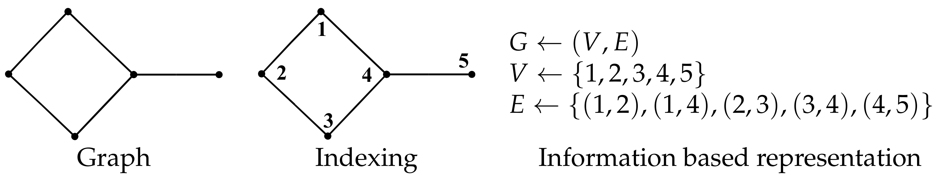
2. Graphs and Their Representation
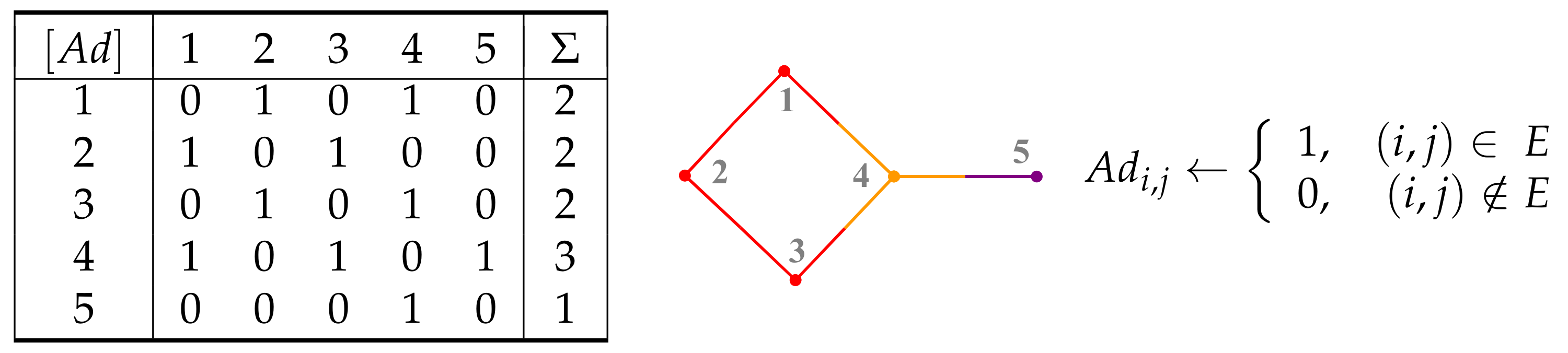
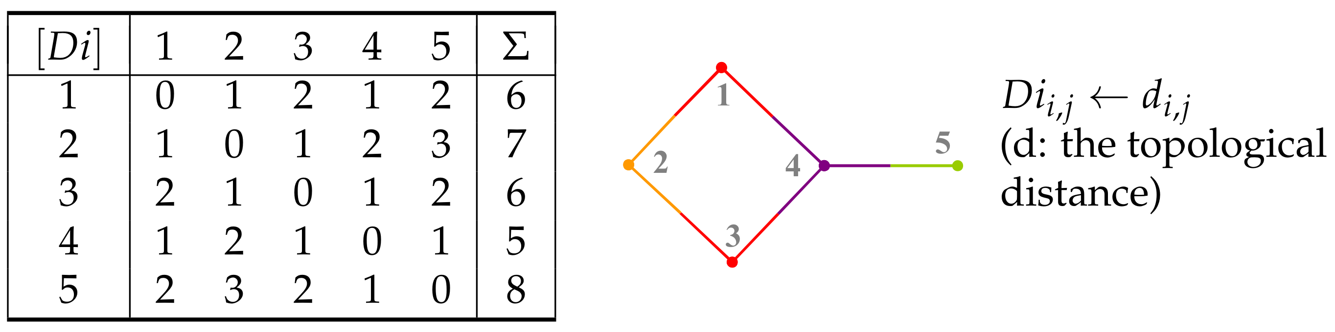
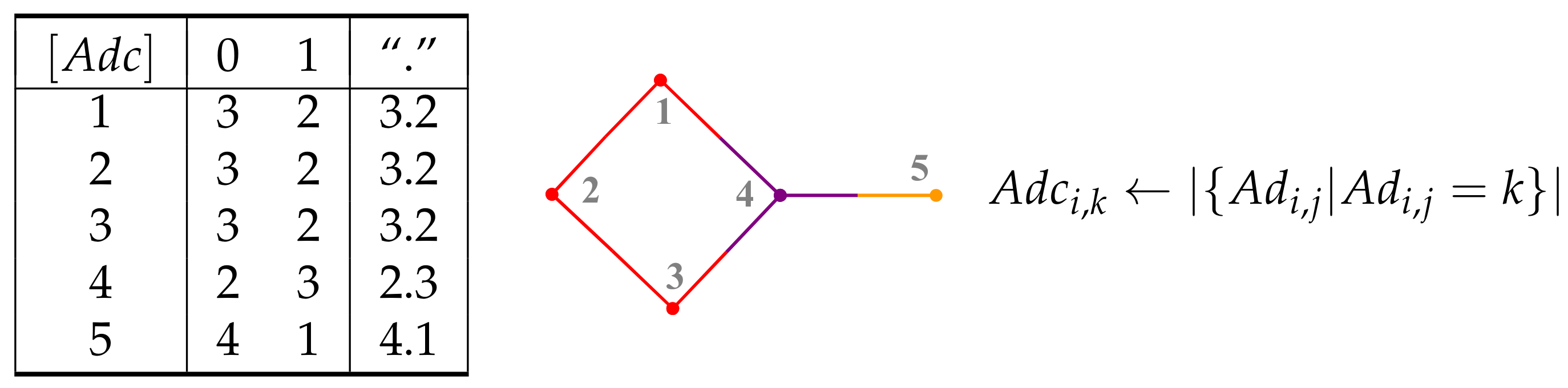
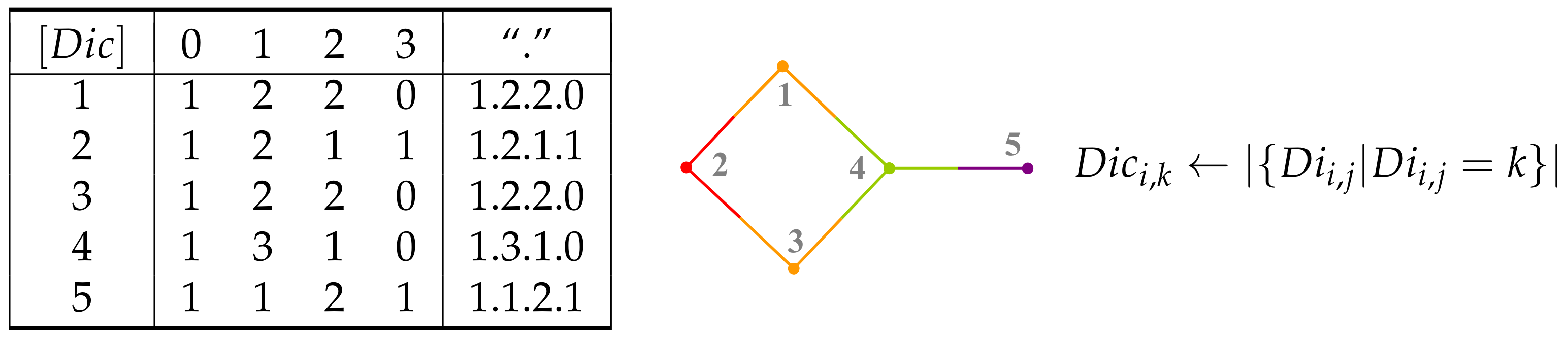
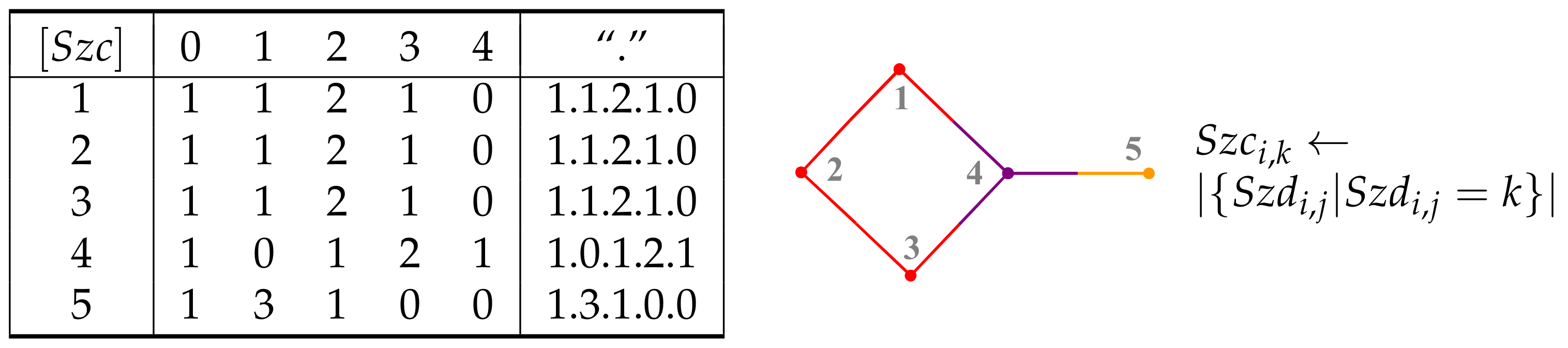
3. Counting Matrices
4. Collecting Sets of Vertices
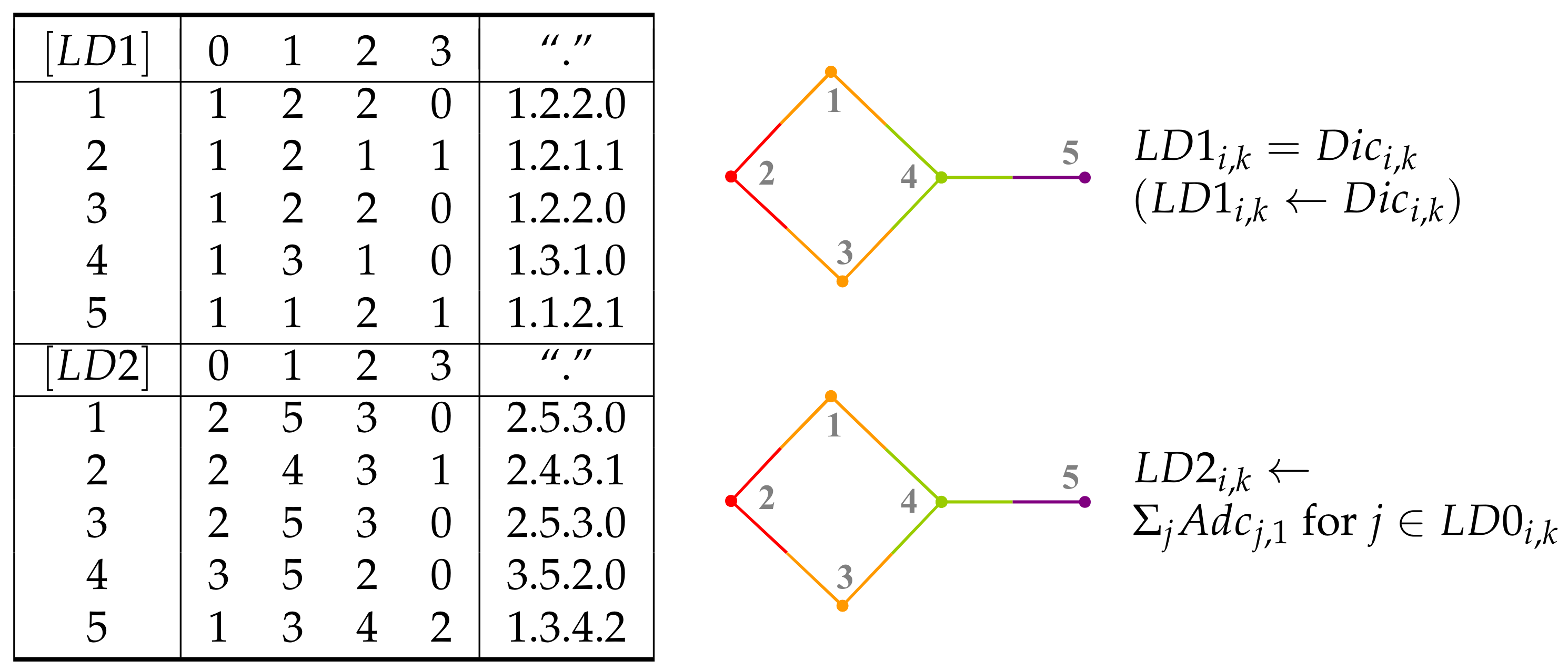
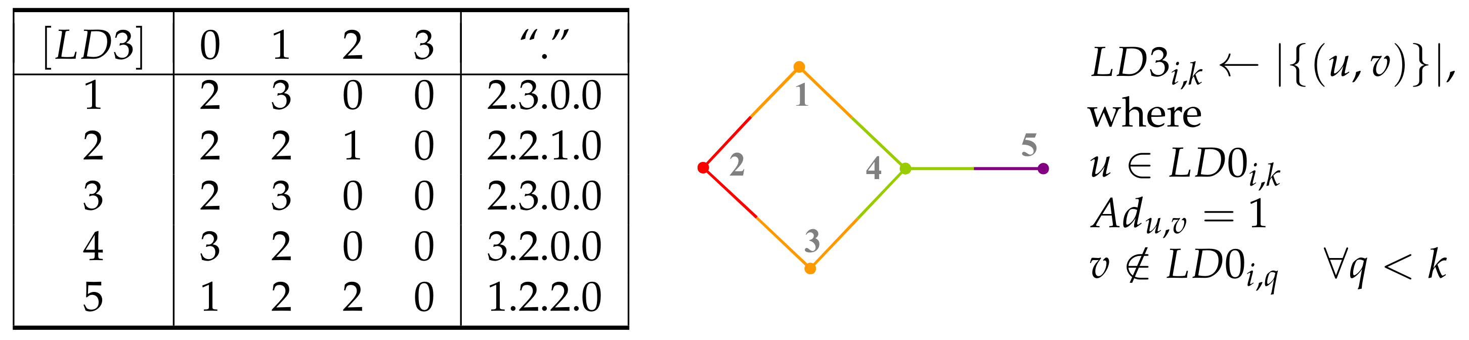
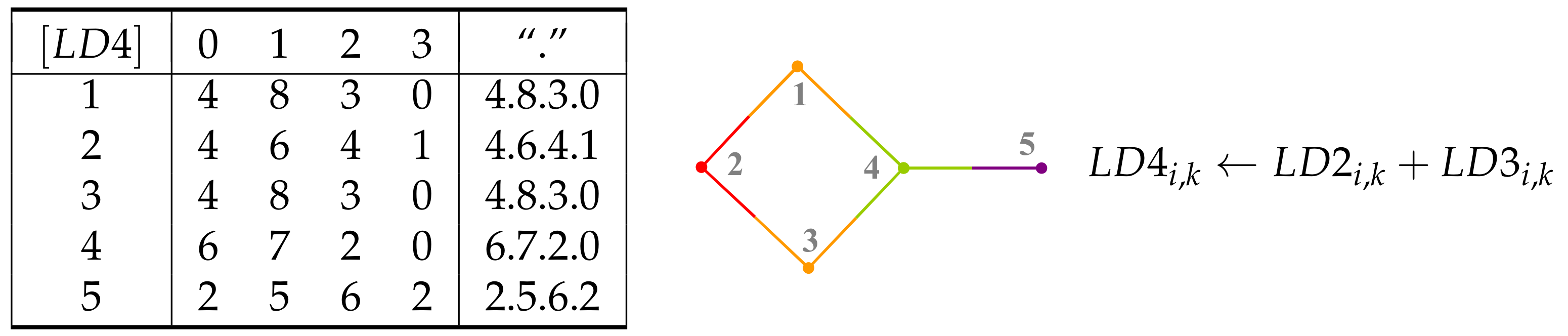
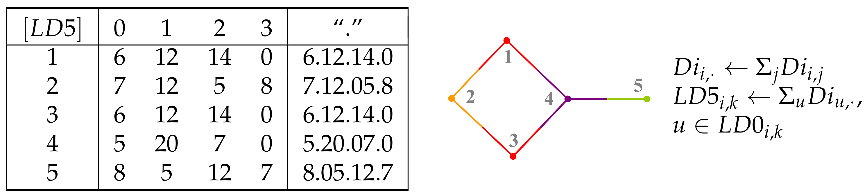
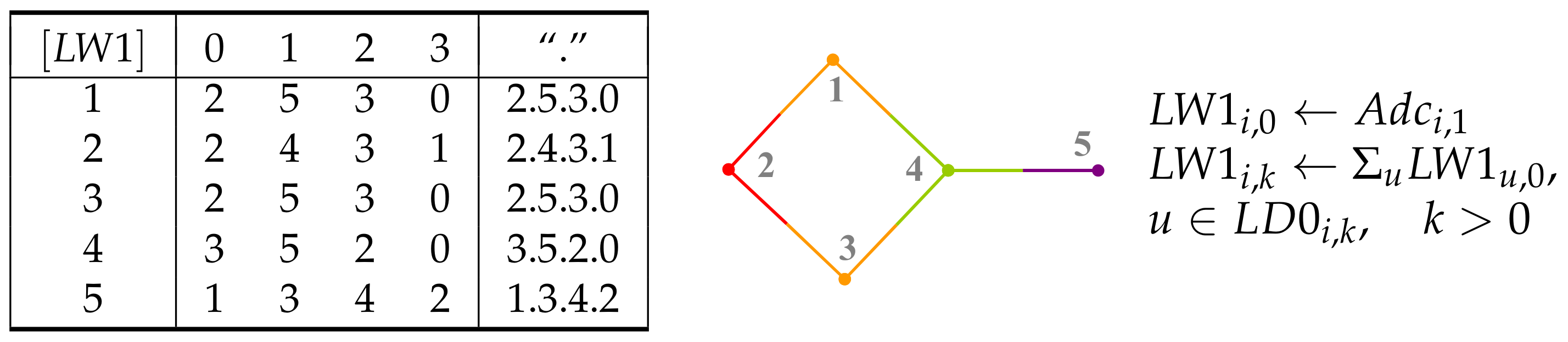
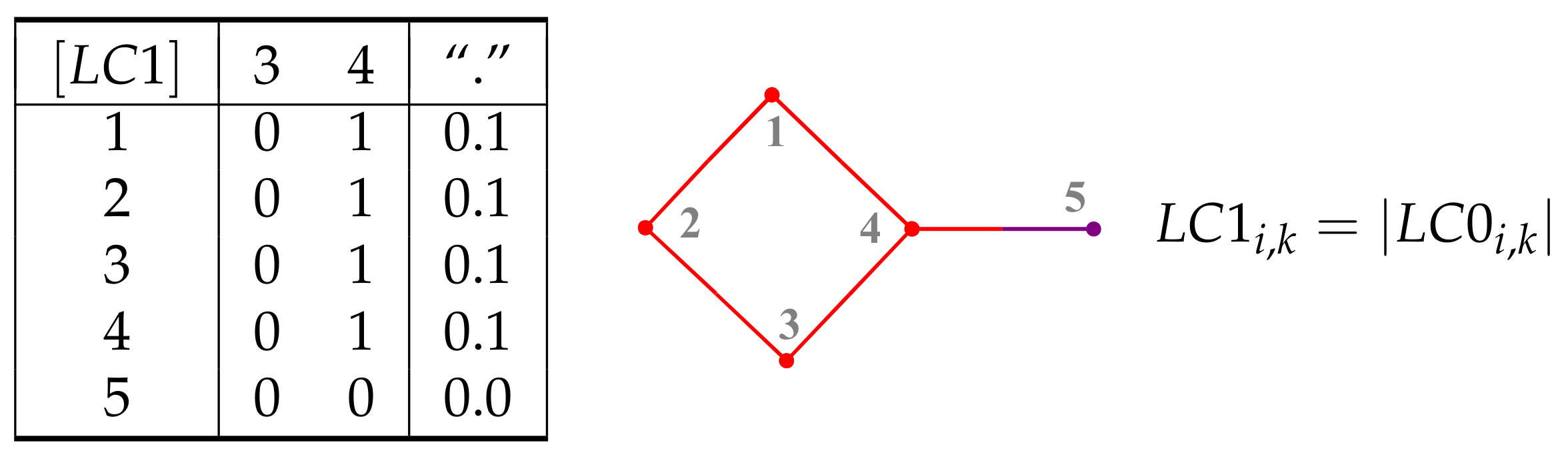
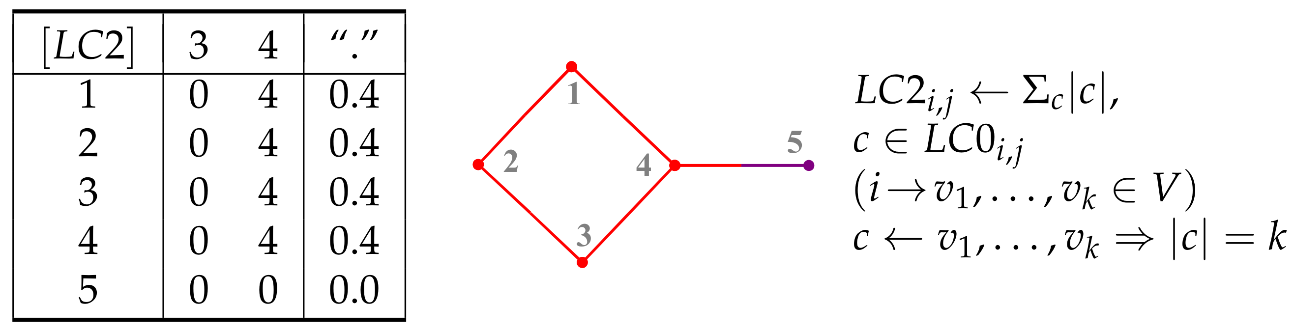
5. Layer Matrices
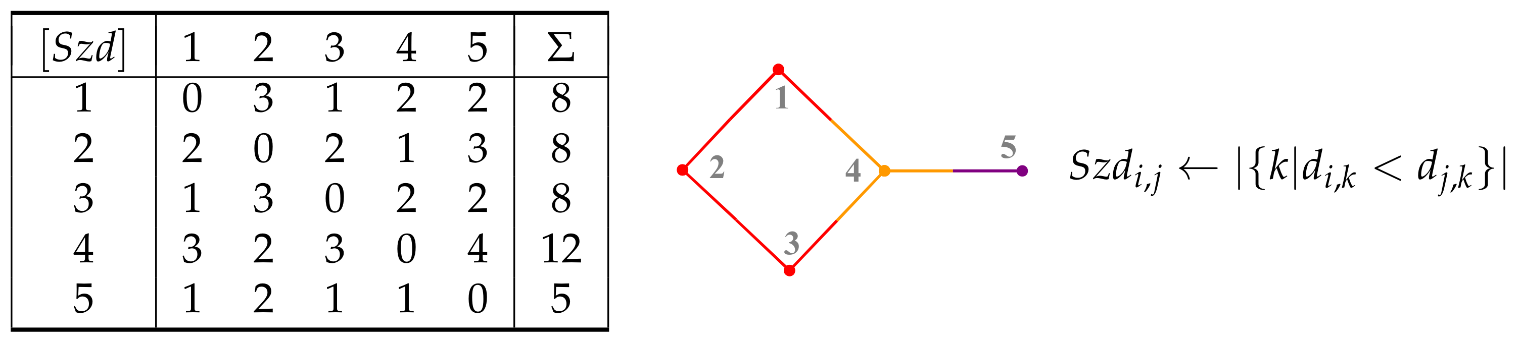
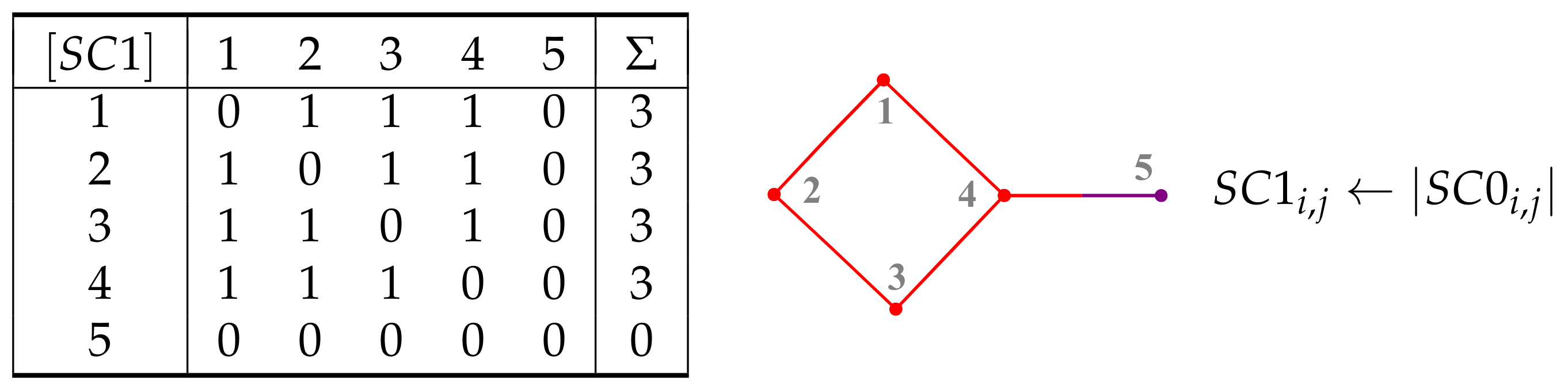
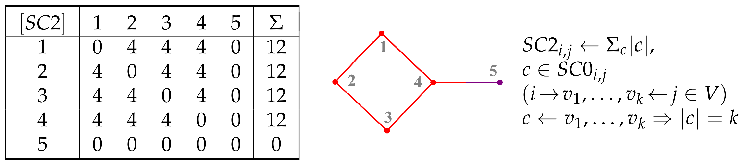
6. Sequence Matrices
7. Paths and Cycles
8. Distinct Partitions Coloring of Vertices
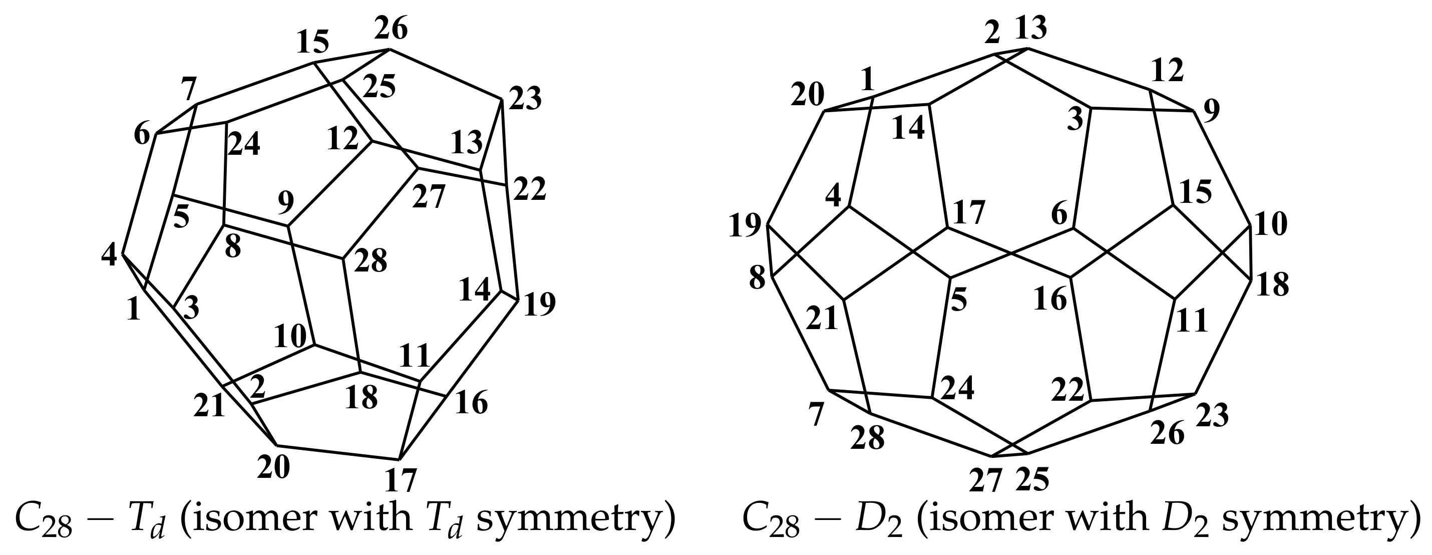
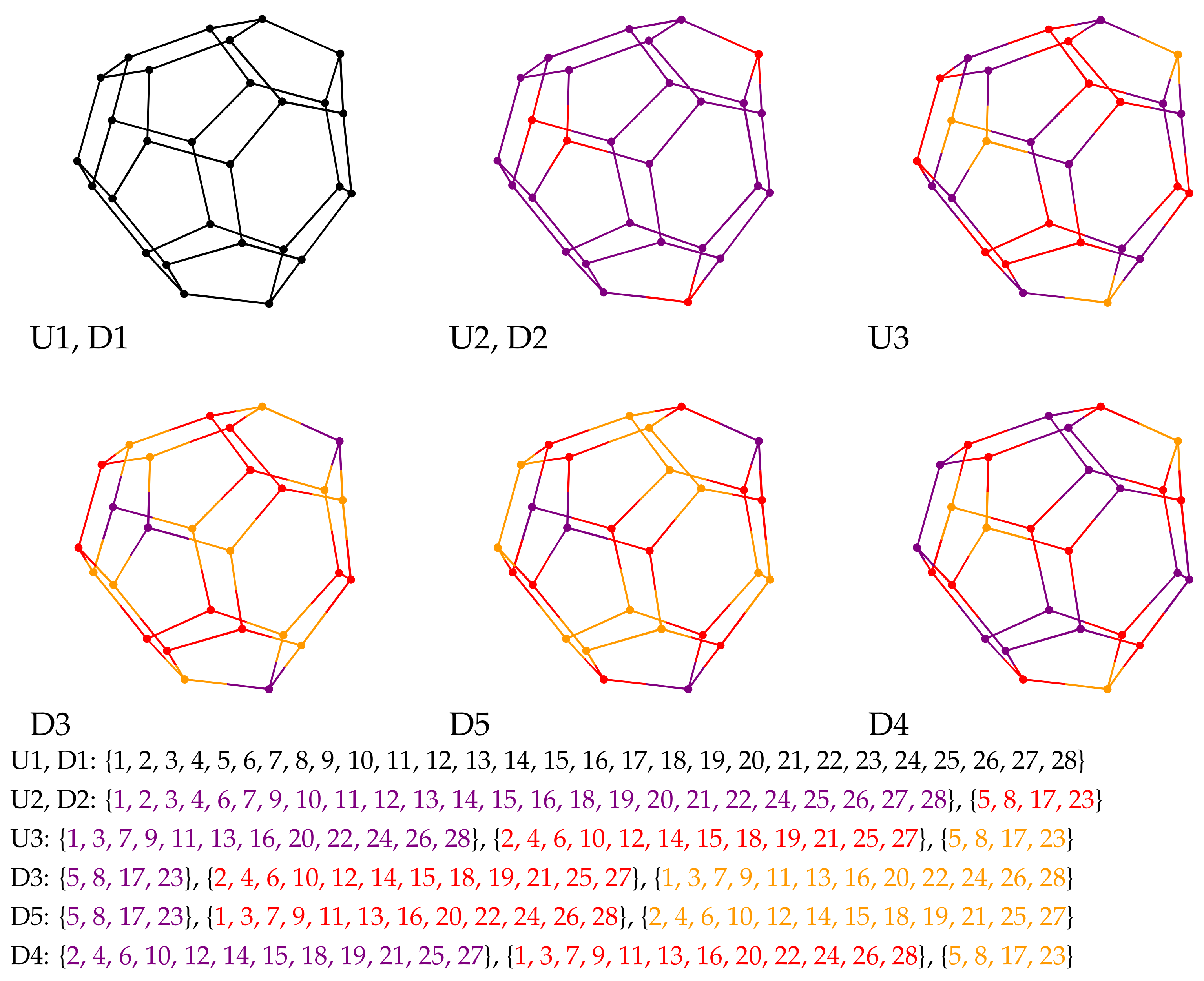
9. Case Study for Isomers of Fullerene
10. Conclusions
Author Contributions
Funding
Institutional Review Board Statement
Informed Consent Statement
Data Availability Statement
Acknowledgments
Conflicts of Interest
Sample Availability
Appendix A. Molecular Graphs and Their Representation
- First three lines—reserved for compound identification
- On fourth line: the number of atoms, the number of bonds, followed by a series of (8) reserved values (numeric and string)
- An block of lines describing on each line one atom: the cartezian coordinates (x, y, and z), the symbol of the atom and a series of (12) reserved fields (numeric)
- An block of lines describing on each line one bond: two numbers acting as indices for the atoms and a third number indicating the bond order, followed by a series of (4) reserved fields (numeric)
- First two lines—reserved for compound identification
- An block of lines describing on each line one atom: type of the fragment, index (numeric), symbol of the atom (1–3 characters), two other columns followed by the cartezian coordinates (x, y, and z)
- An block of lines describing on each line the topology for one atom: atom index followed by the indices of the atoms connected with it
- in between mol and endmol on each line one atom having on the second column the atom index, on the fourth the atom symbol, from column 8 to 11 the cartesian coordinates, on column 12 the number of bonds followed (starting with column 13) by each bond on two columns each (atom index, bond order)
Appendix B. Algorithms

| 0 | 1 | … | ||
|---|---|---|---|---|
| 1 | … | |||
| … | … | … | … | … |
| n | … |
| Algorithm A1 Set adjacency matrix. |
Output:a //a→Ad, Ad—the adjacency matrix () |
| Algorithm A2 Set distance matrix. |
Input:n, a //n←n, a←Ad
Output:d //d→Di, Di—the distance matrix () |
| Algorithm A3 Set graph diameter. |
Input:n, d //n←n, d←Di
Output:e //e→d, d—the diameter (longest distance) |
| Algorithm A4 Set LD2 matrix. |
Input:n, e, f, g //n←n, e←d, f←LD0, g←Dic
Output:h //h→LD2, the LD2 matrix |
| Algorithm A5 Set LD3 matrix. |
Input:n, e, , a, f //n←n, v←tv, a←Ad, e←d, f←LD0
Output:r //r→LD3, the LD3 matrix |
| Algorithm A6 Set LD4 matrix. |
Input:n, e, b, c //n←n, e←d; b←LD2, c←LD3
Output:s //s→LD4, the LD4 matrix |
| Algorithm A7 Set LD5 matrix. |
Input:n, e, d, f //n←n, a←Ad, e←d, g←LD0
Output:h //h→LD5, the LD5 matrix |
| Algorithm A8 Set LkW matrix. |
Input:n, e, a, g //n←n, a←Ad, e←d, g←LD0
Output:h //h→LW, LW the L(1)W..L(e)W matrices |
| Algorithm A9 Set Szeged matrix. |
Input:n, s //n←n, s←Szs
Output:d //d→Szd, Szd—the Szeged matrix |
| Algorithm A10 Set layer sets. |
Input:n, e, m //n←n, e←d, m←Ad, Di,Szd (m—any vertex pair based matrix)
Output:s //s→LA0,LD0,LS0 (s—the layer set of the matrix m) |
| Algorithm A11 Set counting matrix. |
Input:n, m //n←n, m←Ad,Di,Szd (any matrix)
Output:c //c→Adc,Dic,Szc (counting matrix of m) |
| Algorithm A12 Set distances of paths list. |
Input:n, c, d, e //n←n, c←tv; d←Di; e←d
Output:p //p→path, path—the distance paths |
| Algorithm A13 Set cycles list. |
Input:n, a, e, p //n←n, a←Ad, e←d, p←path
Output:c //c→cycle, cycle—the ones no longer than the double of the diameter |
| Algorithm A14 Set distance path sequence and layers. |
Input:n, e, p //n←n, e←d; p←path
Output:s, l //s→SP0, l→LP0—the distance paths sequence and layers |
| Algorithm A15 Set cycle sequence and layers. |
Input:n, c //n←n, c←cycle
Output:s, l //s→SC0, l→LC0—the cycles sequence and layers |
| Algorithm A16 Count and sum for paths and cycles. |
Input:n, //n←n; v←SP0,LP0,SC0, LC0
Output:s, c //c→SP1,LP1,SC1,LC1 (counts), s→SP2,LP2,SC2,LC2 (sums) |
| Algorithm A17 Set Szeged sets. |
Input:n, d //n←n, d←Di
Output:s //s→Szs, Szs—the Szeged sets |
| Algorithm A18 Use of the above algorithms. |
|
References
- Latif, S.; Afzaal, H.; Zafar, N.A. Modelling of Graph-Based Smart Parking System Using Internet of Things. In Proceedings of the 2018 International Conference on Frontiers of Information Technology (FIT), Islamabad, Pakistan, 17–19 December 2018; IEEE: Piscataway, NJ, USA, 2018. [Google Scholar] [CrossRef]
- Kaveh, A. Decomposition for Parallel Computing: Graph Theory Methods. In Computational Structural Analysis and Finite Element Methods; Springer: Cham, Switzerland, 2013; pp. 341–376. [Google Scholar] [CrossRef]
- Bermond, J.-C.; Delorme, C.; Quisquater, J.-J. Strategies for interconnection networks: Some methods from graph theory. J. Parallel Distrib. Comput. 1986, 3, 433–449. [Google Scholar] [CrossRef]
- Mallion, R.B.; Rouvray, D.H. Molecular topology and the Aufbau principle. Mol. Phys. 1978, 36, 125–128. [Google Scholar] [CrossRef]
- Choi, J.-H.; Lee, H.; Choi, H.R.; Cho, M. Graph Theory and Ion and Molecular Aggregation in Aqueous Solutions. Annu. Rev. Phys. Chem. 2018, 69, 125–149. [Google Scholar] [CrossRef] [PubMed]
- Wang, R.; Wu, J.; Qian, Z.; Lin, Z.; He, X. A Graph Theory Based Energy Routing Algorithm in Energy Local Area Network. IEEE Trans. Ind. Inform. 2017, 13, 3275–3285. [Google Scholar] [CrossRef] [Green Version]
- Toscano, L.; Stella, S.; Milotti, E. Using graph theory for automated electric circuit solving. Eur. J. Phys. 2015, 36, 035015. [Google Scholar] [CrossRef] [Green Version]
- Ustun, T.S.; Ayyubi, S. Automated Network Topology Extraction Based on Graph Theory for Distributed Microgrid Protection in Dynamic Power Systems. Electronics 2019, 8, 655. [Google Scholar] [CrossRef] [Green Version]
- Diudea, M.-V.; Gutman, I.; Jäntschi, L. Molecular Topology, 1st ed.; Nova Science: New York, NY, USA, 2001; pp. 1–328. [Google Scholar]
- Joiţa, D.-M.; Jäntschi, L. Extending the Characteristic Polynomial for Characterization of C20 Fullerene Congeners. Mathematics 2017, 5, 84. [Google Scholar] [CrossRef] [Green Version]
- Jäntschi, L. Graph Theory. 2. Vertex Descriptors and Graph Coloring. Leonardo Electron. J. Pract. Technol. 2002, 1, 37–52. [Google Scholar]
- Jäntschi, L. Graph Theory. 1. Fragmentation of Structural Graphs. Leonardo Electron. J. Pract. Technol. 2002, 1, 19–36. [Google Scholar]
- Ballico, E.; Favacchio, G.; Guardo, E.; Milazzo, L.; Thomas, A.C. Steiner Configurations Ideals: Containment and Colouring. Mathematics 2021, 9, 210. [Google Scholar] [CrossRef]
- Buluc, A.; Meyerhenke, H.; Safro, I.; Sanders, P.; Schulz, C. Recent Advances in Graph Partitioning. Lect. Notes Comput. Sci. 2013, 9220, 117–158. [Google Scholar] [CrossRef] [Green Version]
- Choi, D.; Han, J.; Lim, J.; Han, J.; Bok, K.; Yoo, J. Dynamic Graph Partitioning Scheme for Supporting Load Balancing in Distributed Graph Environments. IEEE Access 2021, 9, 65254–65265. [Google Scholar] [CrossRef]
- Miyazawa, F.K.; Moura, P.F.S.; Ota, M.J.; Wakabayashi, Y. Partitioning a graph into balanced connected classes: Formulations, separation and experiments. Eur. J. Oper. Res. 2021, 293, 826–836. [Google Scholar] [CrossRef]
- Miyazawa, F.K.; Moura, P.F.S.; Ota, M.J.; Wakabayashi, Y. Cut and flow formulations for the balanced connected k-partition problem. Lect. Notes Comput. Sci. 2021, 12176, 128–139. [Google Scholar] [CrossRef]
- Bruglieri, M.; Cordone, R. Metaheuristics for the Minimum Gap Graph Partitioning Problem. Comput. Oper. Res. 2021, 132, 105301. [Google Scholar] [CrossRef]
- Bok, K.; Kim, J.; Yoo, J. Dynamic Partitioning Supporting Load Balancing for Distributed RDF Graph Stores. Symmetry 2019, 11, 926. [Google Scholar] [CrossRef] [Green Version]
- Zheng, Z.-Y.; Wang, C.-Y.; Ding, Y.; Li, L.; Li, D. Research on partitioning algorithm based on RDF graph. Concurr. Comput. Pract. Exper. 2021, 33, E5612. [Google Scholar] [CrossRef]
- Wagner, K. Über eine Eigenschaft der ebenen Komplexe. Math. Ann. 1937, 114, 570–590. [Google Scholar] [CrossRef]
- Bodlaender, H.L. A Tourist Guide through Treewidth. Acta Cybern. 1993, 11, 1–21. [Google Scholar]
- Ateskan, E.R.; Erciyes, K.; Dalkilic, M.E. Parallelization of network motif discovery using star contraction. Parallel Comput. 2021, 101, 102734. [Google Scholar] [CrossRef]
- Berry, J.W.; Goldberg, M.K. Path optimization for graph partitioning problems. Discret. Appl. Math. 1999, 90, 27–50. [Google Scholar] [CrossRef] [Green Version]
- Pothen, A.; Simon, H.D.; Liou, K.-P. Partitioning sparse matrices with eigenvectors of graphs. SIAM J. Matrix Anal. Appl. 1990, 11, 430–452. [Google Scholar] [CrossRef]
- Jäntschi, L. The Eigenproblem Translated for Alignment of Molecules. Symmetry 2019, 11, 1027. [Google Scholar] [CrossRef] [Green Version]
- Gupta, A. Fast and effective algorithms for graph partitioning and sparse-matrix ordering. IBM J. Res. Dev. 1997, 41, 171–183. [Google Scholar] [CrossRef]
- Gilbert, J.R.; Miller, G.L.; Teng, S.-H. Geometric mesh partitioning: Implementation and experiments. SIAM J. Sci. Comput. 1998, 19, 2091–2110. [Google Scholar] [CrossRef] [Green Version]
- Karypis, G.; Kumar, V. A fast and high quality multilevel scheme for partitioning irregular graphs. SIAM J. Sci. Comput. 1998, 20, 359–392. [Google Scholar] [CrossRef]
- Kanj, I.; Komusiewicz, C.; Sorge, M.; van Leeuwen, E.J. Parameterized algorithms for recognizing monopolar and 2-subcolorable graphs. J. Comput. Syst. Sci. 2018, 92, 22–47. [Google Scholar] [CrossRef] [Green Version]
- Ahmadi, R.; Nami, S. Investigation of entanglement entropy in cyclic bipartite graphs using computer software. Pramana J. Phys. 2021, 95, 39. [Google Scholar] [CrossRef]
- Hosseinian, S.; Butenko, S. Polyhedral properties of the induced cluster subgraphs. Discrete Appl. Math. 2021, 297, 80–96. [Google Scholar] [CrossRef]
- Nakamura, K.; Araki, T. Partitioning vertices into in- and out-dominating sets in digraphs. Discret. Appl. Math. 2020, 285, 43–54. [Google Scholar] [CrossRef]
- Barbato, M.; Bezzi, D. Monopolar graphs: Complexity of computing classical graph parameters. Discret. Appl. Math. 2021, 291, 277–285. [Google Scholar] [CrossRef]
- Zoltán, F.; Jiang, T.; Kostochka, A.; Mubayi, D.; Verstraëte, J. Partitioning ordered hypergraphs. J. Comb. Theory A 2021, 177, 105300. [Google Scholar] [CrossRef]
- Hellmann, T. Pairwise stable networks in homogeneous societies with weak link externalities. Eur. J. Oper. Res. 2021, 291, 1164–1179. [Google Scholar] [CrossRef]
- McDiarmid, C.; Yolov, N. Recognition of unipolar and generalised split graphs. Algorithms 2015, 8, 46–59. [Google Scholar] [CrossRef] [Green Version]
- Golumbic, M.C.; Lewenstein, M. New results on induced matchings. Discret. Appl. Math. 2000, 101, 157–165. [Google Scholar] [CrossRef] [Green Version]
- Eschen, E.M.; Wang, X. Algorithms for unipolar and generalized split graphs. Discret. Appl. Math. 2014, 162, 195–201. [Google Scholar] [CrossRef] [Green Version]
- Adoni, W.Y.H.; Nahhal, T.; Krichen, M.; El byed, A.; Assayad, I. DHPV: A distributed algorithm for large-scale graph partitioning. J. Big Data 2020, 7, 76. [Google Scholar] [CrossRef] [PubMed]
- Zhang, T.; Gao, Y.; Zheng, B.; Chen, L.; Wen, S.; Guo, W. Towards distributed node similarity search on graphs. World Wide Web 2020, 23, 3025–3053. [Google Scholar] [CrossRef]
- Schaudt, O. On weighted efficient total domination. J. Discret. Alg. 2012, 10, 61–69. [Google Scholar] [CrossRef] [Green Version]
- Schaeffer, S.E. Graph clustering. Comput. Sci. Rev. 2007, 1, 27–64. [Google Scholar] [CrossRef]
- De Freitas, R.; Dias, B.; Maculan, N. Szwarcfiter, J. On distance graph coloring problems. Int. Trans. Oper. Res. 2021, 28, 1213–1241. [Google Scholar] [CrossRef]
- Slamin, S.; Adiwijaya, N.O.; Hasan, M.A.; Dafik, D.; Wijaya, K. Local Super Antimagic Total Labeling for Vertex Coloring of Graphs. Symmetry 2020, 12, 1843. [Google Scholar] [CrossRef]
- Šurimová, M.; Lužar, B.; Madaras, T. Adynamic coloring of graphs. Discret. Appl. Math. 2020, 284, 224–233. [Google Scholar] [CrossRef]
- Dokeroglu, T.; Sevinc, E. Memetic Teaching–Learning-Based Optimization algorithms for large graph coloring problems. Eng. Appl. Artif. Intell. 2021, 102, 104282. [Google Scholar] [CrossRef]
- Zaker, M. A New Vertex Coloring Heuristic and Corresponding Chromatic Number. Algorithmica 2020, 82, 2395–2414. [Google Scholar] [CrossRef]
- Lehner, F.; Smith, S.M. On symmetries of edge and vertex colourings of graphs. Discret. Math. 2020, 343, 111959. [Google Scholar] [CrossRef]
- Ahmadi, B.; Alinaghipour, F.; Shekarriz, M.H. Number of distinguishing colorings and partitions. Discret. Math. 2020, 343, 111984. [Google Scholar] [CrossRef]
- Raza, Z.; Essa, K.; Sukaiti, M. M-Polynomial and Degree Based Topological Indices of Some Nanostructures. Symmetry 2020, 12, 831. [Google Scholar] [CrossRef]
- Harary, F.; Paper, H.H. Toward a General Calculus of Phonemic Distribution. Language 1957, 33, 143. [Google Scholar] [CrossRef]
- Giffler, B.; Thompson, G.L. Algorithms for Solving Production-Scheduling Problems. Oper. Res. 1960, 8, 487–503. [Google Scholar] [CrossRef]
- Györi, I.; Joó, G. Computer-aided acoustic analysis of reciprocating compressor pipeline systems. Eng. Comput. 1987, 3, 21–33. [Google Scholar] [CrossRef]
- Lee, S.; Liu, Z.; Kim, C. An Agent Using Matrix for Backward Path Search on MANET. Lect. Notes Comput. Sci. 2008, 4953, 203–211. [Google Scholar] [CrossRef]
- Hayward, C.L. Biotic Communities of the Wasatch Chaparral, Utah. Ecol. Monogr. 1948, 18, 473–506. [Google Scholar] [CrossRef]
- Dobrynin, A.A. Graphs with coincident complete matrices of layers. Vychisl. Sist. 1987, 119, 3–12. [Google Scholar]
- Dobrynin, A.A. Graphs with coincident chain-like matrices of layers. Vychisl. Sist. 1987, 119, 13–33. [Google Scholar]
- Skorobogatov, V.A.; Dobrynin, A.A. Metric analysis of graphs. MATCH-Commun. Math. Chem. 1988, 23, 105–151. [Google Scholar]
- Dobrynin, A.A. Regular graphs having the same path layer matrix. J. Graph. Theory 1990, 14, 141–148. [Google Scholar] [CrossRef]
- Dobrynin, A.A. Cubic graphs with 62 vertices having the same path layer matrix. J. Graph. Theory 1993, 17, 1–4. [Google Scholar] [CrossRef]
- Diudea, M.V.; Horvath, D.; Kacsó, I.E.; Minailiuc, O.M.; Parv, B. Molecular topology. VIII: Centricities in molecular graphs. The mollen algorithm. J. Math. Chem. 1992, 11, 259–270. [Google Scholar] [CrossRef]
- Yuansheng, Y.; Xiaohui, L.; Zhiqiang, C.; Weiming, L. 4-Regular Graphs without Cut-Vertices having the Same Path Layer Matrix. J. Graph. Theory 2003, 44, 304–311. [Google Scholar] [CrossRef]
- Lungu, C.N. C-C chemokine receptor type 3 inhibitors: Bioactivity prediction using local vertex invariants based on thermal conductivity layer matrix. Stud. Univ. Babes-Bolyai Chem. 2018, 63, 177–188. [Google Scholar] [CrossRef]
- Hosoya, H. Topological Index. A Newly Proposed Quantity Characterizing the Topological Nature of Structural Isomers of Saturated Hydrocarbons. Bull. Chem. Soc. Jpn. 1971, 44, 2332–2339. [Google Scholar] [CrossRef] [Green Version]
- Hosoya, H. On some counting polynomials in chemistry. Discret. Appl. Math. 1988, 19, 239–257. [Google Scholar] [CrossRef] [Green Version]
- Pólya, G. Kombinatorische Anzahlbestimmungen für Gruppen, Graphen und chemische Verbindungen. Acta Math. 1937, 68, 145–254. [Google Scholar] [CrossRef]
- Diudea, M.V. Omega polynomial in twisted/chiral polyhex tori. J. Math. Chem. 2009, 45, 309–315. [Google Scholar] [CrossRef]
- Diudea, M.V. Hosoya Polynomial in Tori. MATCH-Commun. Math. Chem. 2002, 45, 109–122. [Google Scholar]
- Müller, J. On the multiplicity-free actions of the sporadic simple groups. J. Algebra 2008, 320, 910–926. [Google Scholar] [CrossRef] [Green Version]
- Fujita, S. Symmetry-itemized enumeration of cubane derivatives as three-dimensional entities by the fixed-point matrix method of the USCI approach. Bull. Chem. Soc. Jpn. 2011, 84, 1192–1207. [Google Scholar] [CrossRef]
- Ştefu, M.V.; Pârvan-Moldovan, A.; Kooperazan-Moftakhar, F.; Diudea, M.V. Topological symmetry of C60-related multi-shell clusters. MATCH-Commun. Math. Chem. 2015, 74, 273–284. [Google Scholar]
- Dinca, M.F.; Ciger, S.; Ştefu, M.V.; Gherman, F.; Miklos, K.; Nagy, C.L.; Ursu, O.; Diudea, M.V. Stability prediction in C40 fullerenes. Carpathian J. Math. 2004, 20, 211–221. [Google Scholar]
- Diudea, M.V.; Minailiuc, O.M.; Balaban, A.T. Molecular topology. IV. Regressive vertex degrees (new graph invariants) and derived topological indices. J. Comput. Chem. 1991, 12, 527–535. [Google Scholar] [CrossRef]
- Balaban, A.T.; Diudea, M.V. Real Number Vertex Invariants: Regressive Distance Sums and Related Topological Indices. J. Chem. Inf. Comput. Sci. 1993, 33, 421–428. [Google Scholar] [CrossRef]
- Diudea, M.V. Molecular Topology. 16. Layer Matrixes in Molecular Graphs. J. Chem. Inf. Comput. Sci. 1994, 34, 1064–1071. [Google Scholar] [CrossRef]
- Wiener, H. Structural Determination of Paraffin Boiling Point. J. Am. Chem. Soc. 1947, 69, 17–20. [Google Scholar] [CrossRef]
- Morgan, H. The Generation of a Unique Machine Description for Chemical Structures. A Technique Developed at Chemical Abstracts Service. J. Chem. Doc. 1965, 5, 107–113. [Google Scholar] [CrossRef]
- Knuth, D. Postscript about NP-hard problems. ACM SIGACT News 1974, 6, 15–16. [Google Scholar] [CrossRef]
- Pan, Y.; Morisako, S.; Aoyagi, S.; Sasamori, T. Generation of Bis(ferrocenyl)silylenes from Siliranes. Molecules 2020, 25, 5917. [Google Scholar] [CrossRef]
- Thompson, B.C.; Fréchet, J.M.J. Polymer-fullerene composite solar cells. Angew. Chem. Int. Ed. 2008, 47, 58–77. [Google Scholar] [CrossRef] [PubMed]
- Al-Jumaili, A.; Alancherry, S.; Bazaka, K.; Jacob, M.V. Review on the Antimicrobial Properties of Carbon Nanostructures. Materials 2017, 10, 1066. [Google Scholar] [CrossRef]
- De Stefani, A.; Bruno, G.; Preo, G.; Gracco, A. Application of Nanotechnology in Orthodontic Materials: A State-of-the-Art Review. Dent. J. 2020, 8, 126. [Google Scholar] [CrossRef] [PubMed]
- Došlić, T. All Pairs of Pentagons in Leapfrog Fullerenes Are Nice. Mathematics 2020, 8, 2135. [Google Scholar] [CrossRef]
- Da Ros, T.; Prato, M. Medicinal chemistry with fullerenes and fullerene derivatives. Chem. Commun. 1999, 663–669. [Google Scholar] [CrossRef]


| 0 | 1 | |
|---|---|---|
| 1 | {1, 3, 5} | {2, 4} |
| 2 | {2, 4, 5} | {1, 3} |
| 3 | {1, 3, 5} | {2, 4} |
| 4 | {2, 4} | {1, 3, 5} |
| 5 | {1, 2, 3, 5} | {4} |
| 0 | 1 | 2 | 3 | |
|---|---|---|---|---|
| 1 | {1} | {2, 4} | {3, 5} | {} |
| 2 | {2} | {1, 3} | {4} | {5} |
| 3 | {3} | {2, 4} | {1, 5} | {} |
| 4 | {4} | {1, 3, 5} | {2} | {} |
| 5 | {5} | {4} | {1, 3} | {2} |
| 0 | 1 | 2 | 3 | 4 | |
|---|---|---|---|---|---|
| 1 | {1} | {3} | {4, 5} | {2} | {} |
| 2 | {2} | {4} | {1, 3} | {5} | {} |
| 3 | {3} | {1} | {4, 5} | {2} | {} |
| 4 | {4} | {} | {2} | {1, 3} | {5} |
| 5 | {5} | {1, 3, 4} | {2} | {} | {} |
| 1 | 2 | 3 | 4 | 5 | |
|---|---|---|---|---|---|
| 1 | {} | {1 2} | {1 4 3, 1 2 3} | {1 4} | {1 4 5} |
| 2 | {2 1} | {} | {2 3} | {2 3 4, 2 1 4} | {2 1 4 5, 2 3 4 5} |
| 3 | {3 4 1, 3 2 1} | {3 2} | {} | {3 4} | {3 4 5} |
| 4 | {4 1} | {4 3 2, 4 1 2} | {4 3} | {} | {4 5} |
| 5 | {5 4 1} | {5 4 1 2, 5 4 3 2} | {5 4 3} | {5 4} | {} |
| 0 | 1 | 2 | 3 | |
|---|---|---|---|---|
| 1 | {} | {1 2, 1 4} | {1 4 3, 1 4 5, 1 2 3} | {} |
| 2 | {} | {2 1, 2 3} | {2 3 4, 2 1 4} | {2 1 4 5, 2 3 4 5} |
| 3 | {} | {3 2, 3 4} | {3 4 5, 3 4 1, 3 2 1} | {} |
| 4 | {} | {4 1, 4 3, 4 5} | {4 3 2, 4 1 2} | {} |
| 5 | {} | {5 4} | {5 4 3, 5 4 1} | {5 4 1 2, 5 4 3 2} |
| 1 | 2 | 3 | 4 | 5 | |
|---|---|---|---|---|---|
| 1 | {} | {1 2 3 4} | {1 2 3 4} | {1 2 3 4} | {} |
| 2 | {1 2 3 4} | {} | {1 2 3 4} | {1 2 3 4} | {} |
| 3 | {1 2 3 4} | {1 2 3 4} | {} | {1 2 3 4} | {} |
| 4 | {1 2 3 4} | {1 2 3 4} | {1 2 3 4} | {} | {} |
| 5 | {} | {} | {} | {} | {} |
| 3 | 4 | |
|---|---|---|
| 1 | {} | {1 2 3 4} |
| 2 | {} | {1 2 3 4} |
| 3 | {} | {1 2 3 4} |
| 4 | {} | {1 2 3 4} |
| 5 | {} | {} |
| 1 | 2 | 3 | 4 | 5 | |
|---|---|---|---|---|---|
| 1 | {} | {1, 4, 5} | {1} | {1, 2} | {1, 2} |
| 2 | {2, 3} | {} | {1, 2} | {2} | {1, 2, 3} |
| 3 | {3} | {3, 4, 5} | {} | {2, 3} | {2, 3} |
| 4 | {3, 4, 5} | {4, 5} | {1, 4, 5} | {} | {1, 2, 3, 4} |
| 5 | {5} | {4, 5} | {5} | {5} | {} |
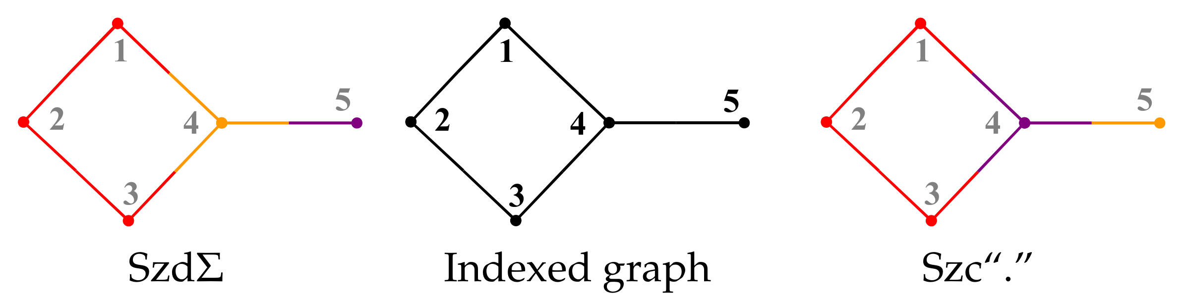
| Vertices | “.” | |
|---|---|---|
| 1 | 8 | 1.1.2.1.0 |
| 2 | 8 | 1.1.2.1.0 |
| 3 | 8 | 1.1.2.1.0 |
| 4 | 12 | 1.0.1.2.1 |
| 5 | 5 | 1.3.1.0.0 |
| Order of the Vertices Sets Is Relevant | Classifier (from ) | Order of the Vertices Sets Is Not Relevant |
|---|---|---|
| {5}, {1, 2, 3}, {4} | Ad, Szd | {1, 2, 3}, {4}, {5} |
| {4}, {1, 2, 3}, {5} | Adc, Szc | |
| {4}, {1, 3}, {2}, {5} | Di, LD5 | {1, 3}, {2}, {4}, {5} |
| {5}, {2}, {1, 3}, {4} | Dic, LD1, LD2, LD3, LD4, LW1, LW2, LP1, LP2 | |
| {5}, {1, 3}, {2}, {4} | LW3 | |
| {4}, {1,3}, {5}, {2} | SP2 | |
| {1, 3, 4, 5}, {2} | SP1 | {1, 3, 4, 5}, {2} |
| {5}, {1, 2, 3, 4} | SC1, SC2, LC1, LC2 | {1, 2, 3, 4}, {5} |
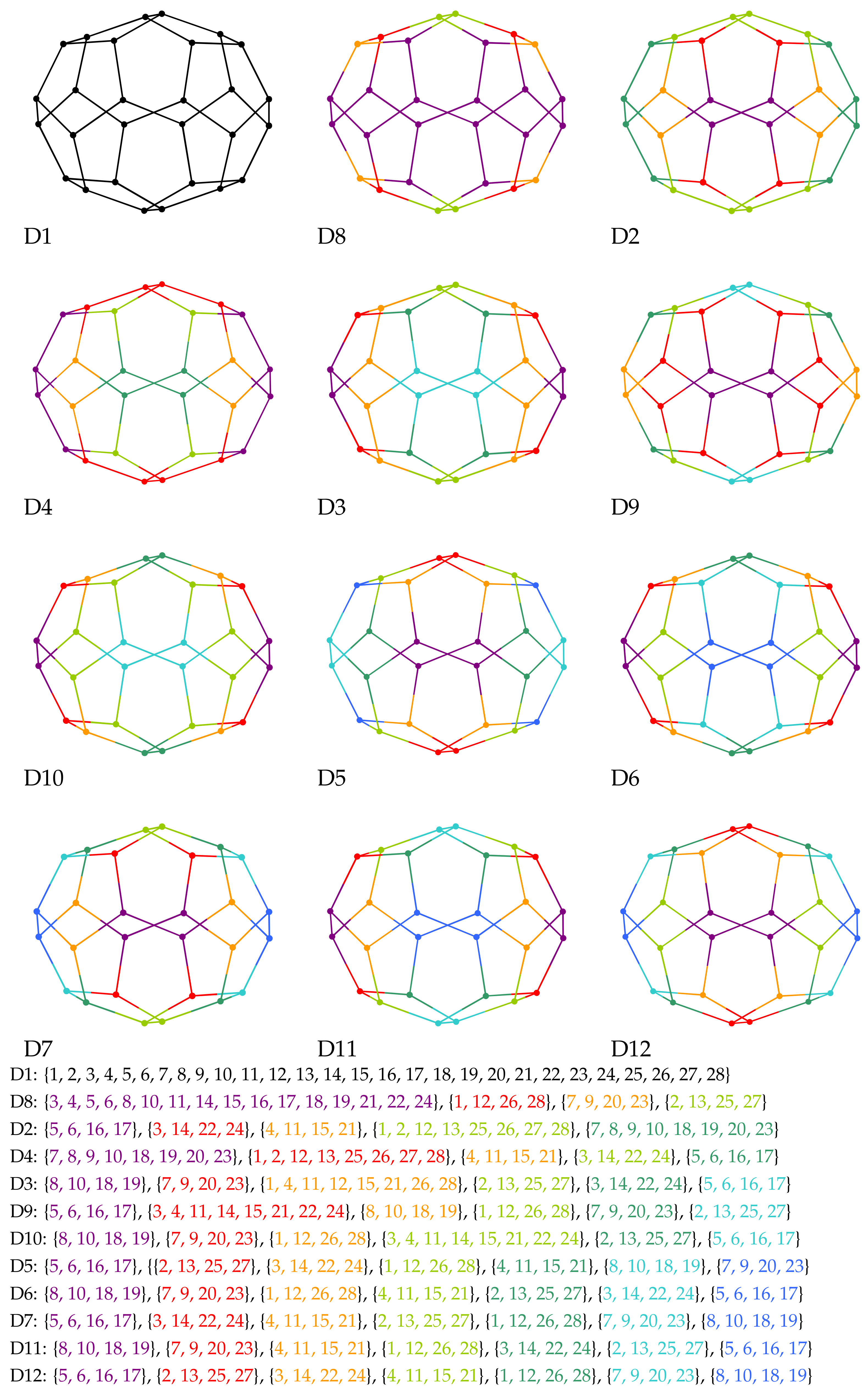
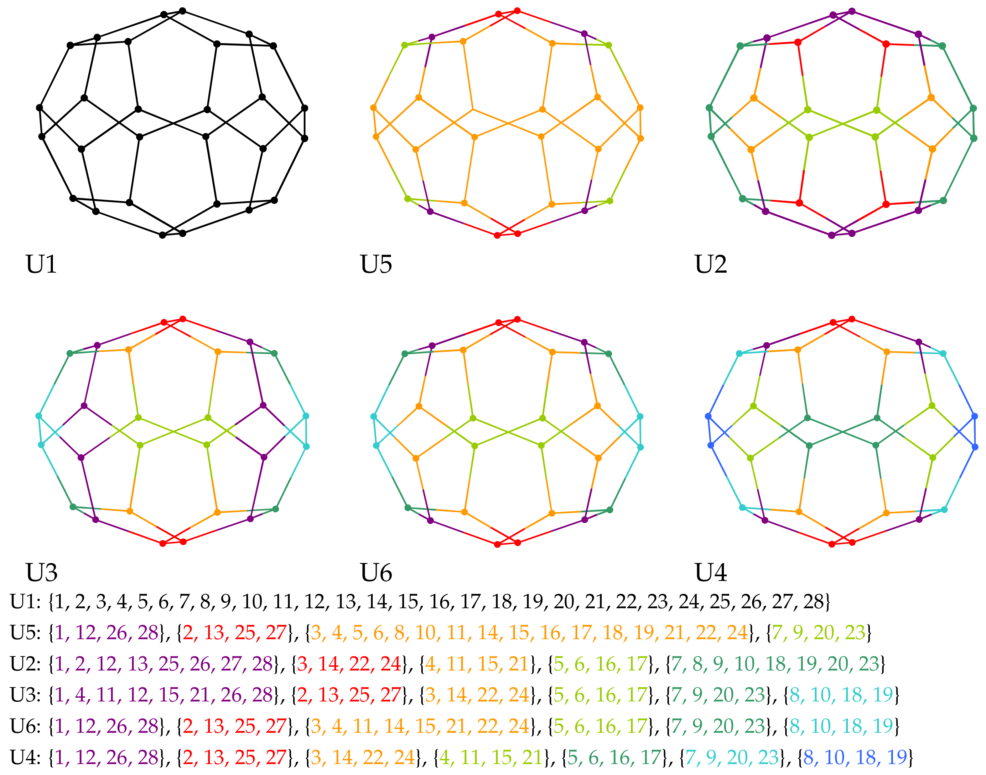
| Order Is Relevant | Classifiers | Order Is Not Relevant |
|---|---|---|
| D1 | Ad, Adc | U1 |
| D2 | Di | U2 |
| D4 | Dic, LD1, LD2, LW1, LW2, LW3, LW4, LW5, LW6 | |
| D3 | Szd | U3 |
| D5 | Szc | U4 |
| D6 | LD3, LD4 | |
| D7 | LD5 | |
| D11 | SC1, SC2 | |
| D12 | LC1, LC2 | |
| D8 | SP1 | U5 |
| D9 | SP2 | U6 |
| D10 | LP1, LP2 |
| Order Is Relevant | Classifiers | Order Is Not Relevant |
|---|---|---|
| D1 | Ad, Adc | U1 |
| D2 | Di | U2 |
| D3 | Dic, LD1, LD2, LW1, LW2, LW3, LW4, LW5, LW6, Szd | U3 |
| D4 | Szc, LD5, SP1, SP2, SC1, SC2, LC1, LC2 | |
| D5 | LD3, LD4, LP1, LP2 |
Publisher’s Note MDPI stays neutral with regard to jurisdictional claims in published maps and institutional affiliations. |
© 2021 by the authors. Licensee MDPI, Basel, Switzerland. This article is an open access article distributed under the terms and conditions of the Creative Commons Attribution (CC BY) license (https://creativecommons.org/licenses/by/4.0/).
Share and Cite
Tomescu, M.A.; Jäntschi, L.; Rotaru, D.I. Figures of Graph Partitioning by Counting, Sequence and Layer Matrices. Mathematics 2021, 9, 1419. https://doi.org/10.3390/math9121419
Tomescu MA, Jäntschi L, Rotaru DI. Figures of Graph Partitioning by Counting, Sequence and Layer Matrices. Mathematics. 2021; 9(12):1419. https://doi.org/10.3390/math9121419
Chicago/Turabian StyleTomescu, Mihaela Aurelia, Lorentz Jäntschi, and Doina Iulia Rotaru. 2021. "Figures of Graph Partitioning by Counting, Sequence and Layer Matrices" Mathematics 9, no. 12: 1419. https://doi.org/10.3390/math9121419