1. Introduction
The PID controllers are widespread in many industries and are frequently included in embedded solutions [
1,
2,
3,
4]. This is not surprising, since the basic PID control algorithm is very simple and the control performance, when the controller is tuned appropriately, is usually very good. However, the control performance can be improved by increasing the controller order. The improvement depends on the process order. While the first-order process can be efficiently controlled by the PI controller and the second-order process by the PID controller, the control efficiency for higher-order processes can be improved by increasing the controller order beyond the PID control.
In practice the PI controllers are used more often than the PID controllers, since the latter significantly increase the controller output noise. Naturally, with higher degrees of controllers, the problem becomes aggravated. Therefore, the appropriate higher-order controller filter is inevitable in practical applications.
For easier classification of the HO-PID controllers according to the controller (m) and filter (
n) order, let us denote them as
. A general
controller transfer function
GCF(
s) can be defined as follows:
where
K−1,
K0,
K1, …
Km are controller gains, and
GF(
s) is the binomial filter with filter time constant
TF. In practical applications, in order to limit the higher-frequency controller output noise,
n ≥
m. Note that
denotes the PI controller (
KI =
K−1,
KP =
K0) and
denotes the PID controller (
KI =
K−1,
KP =
K0,
KD =
K1) with the first-order filter (
n = 1).
Several tuning methods for HO-PID controllers have been proposed so far. The majority of them are made for proportional-integrative-derivative-accelerative (PIDA) controllers (
). The controller structure is either 1 degree of freedom (1-DOF) [
5,
6,
7,
8,
9,
10,
11,
12,
13,
14,
15,
16,
17,
18,
19,
20] or 2 degrees of freedom (2-DOF) [
21,
22,
23] which can optimise the tracking and control performance.
The tuning methods for the mentioned PIDA controllers are derived either for the first-order process with delay [
20,
22,
23], third order process [
5,
11,
13,
14,
21], first-order double integrating process [
5,
11,
16], second-order integrating process [
8,
9,
11,
16], double integrating process with time delay [
10], fourth-order system [
18], for different types of process models [
6,
17,
18] or for the automatic voltage regulator (AVR) in the generator excitation system [
7,
15,
19]. Unfortunately, only a few of the mentioned PIDA controller tuning methods take into account the controller filter in the controller design stage [
5,
6,
7,
10,
15,
23]. Therefore, the practical implementation of other PIDA tuning methods remains questionable.
Besides PIDA controllers, some higher-order controller tuning methods also exist [
24,
25,
26,
27]. The tuning method for the
controller (the controller filter is not considered), where the controlled process is a model of the ship power plant, including the heat exchanger, is given in [
24]. The method optimises the IAE for disturbance rejection while limiting the peak of the closed-loop amplitude frequency response.
Tuning methods for even higher-order controllers (
m > 3) were developed for the integrating process model with a time delay (IPTD) [
25,
26,
27]. Although the type of the process model seems to be limited, we have to mention that many stable process models can be modelled as IPTD processes [
1]. For HO-PID control of stable time-delayed processes, a new method was also proposed by generalizing Skogestad’s method SIMC [
28]. The basic version is based on the approximation of processes by transfer functions with multiple time constants (obtained, for example, by an appropriate identification method); however, a suitable model can also be obtained from a more general description of the process reduced by the modified “half-rule” method [
29]. Although not specifically designed for HO-PID controllers, we should also mention that the tuning approach is based on the design of multiple dominant closed-loop poles for delayed processes, applied to the PI and PID controllers [
30], which can be easily extended to HO-PID controllers.
The developed tuning methods for the controllers reveal that the HO-PID controllers can be much more efficient than the ordinary PID controllers without significant increase of the controller output noise.
This paper presents the controller and filter tuning method, which is based on the parametric or the non-parametric process description. It means that the process can be given by the general transfer function (of the arbitrary order and time delay) or by the process input and output time-responses during the steady-state change of the process. The only user-defined parameters will be the controller (m) and the filter (n) order and the desired high-frequency gain of the controller. As will be shown later, the controller parameters will be calculated analytically.
Therefore, the main advantages of the proposed method are the flexibility of the process description (the process model is not required), simple specifications by the user and simple calculation of the controller and filter parameters.
The content of the paper is as follows. The tuning method for the
controllers is covered in
Section 2. The calculation of the controller and controller filter time constant, according to the desired closed-loop high-frequency gain, is derived in
Section 3. The comparison with some other tuning methods is carried out in
Section 4. The paper concludes with
Section 5.
2. HO-PID Controller Tuning
The HO-PID controller parameters will be derived according to the magnitude optimum multiple integration (MOMI) tuning method, which is based on the magnitude optimum (MO) criteria [
31,
32,
33,
34,
35,
36,
37]. The main advantages of the MOMI method are that it combines frequency-domain MO tuning criterion (providing a fast and non-oscillatory closed-loop process output response) with the time-domain method of moments (the calculation of the process characteristic areas directly from the process time responses).
The process
The general order process transfer function with time delay is defined by the following expression:
where
KPR is the process gain,
Tdel is the process time delay and
a1 to
ap and
b1 to
br are the process dynamic parameters. To simplify the derivation, let us assume that the process transfer function is developed into an infinite Taylor series around
s = 0:
where
GPk are the
k-th derivatives of the
GP(
s) over s around
s = 0. The moments can be calculated from the process impulse response
h(
t) in the following way [
1,
38]:
Besides measuring the process impulse response, the moments can also be calculated from the process steady-state change by measuring the process input and output time responses [
32,
34]. By integrating the process input and output time responses, the so-called characteristic areas
Ak are obtained, which are related to the process moments as follows:
The process transfer function, based on the characteristic areas, can be derived from (3) and (5) as follows:
Since the calculation of the mentioned areas from the process input and output time responses, during arbitrary steady-state change, are already covered in detail in [
36], it will not be repeated herein.
The process moments (4) and, therefore, the characteristic areas
Ak (5), can also be calculated from the process transfer function (2) by calculating the derivatives of
GP(
s) over
s around
s = 0. The result is the following [
32,
34]:
Therefore, the characteristic areas in expression (6) can be calculated either from the process time response or from the process transfer function. This is a very important advantage, since the actual process model can be used, but is not required.
In order to simplify the derivation of the controller parameters, the controller binomial filter
GF(
s) (1) will be considered as a part of the process. Since the above areas are calculated for the process without the filter, the areas
Ai should be modified, accordingly. If the filter
GF(
s) (1) is added to the process (2) and developed into a Taylor series, it can be derived that the new areas, denoted by
AiF, can be simply calculated as:
Note that n is the binomial filter order (1). Naturally, the chosen size of the matrix and the vectors depends on the number of the required areas.
Note that the characteristic areas with the included controller filter can be obtained a-posteriori, when the process areas Ai are already measured either from the process time response (5) or calculated from the process transfer function (7).
For further reference, please note that the process areas with the included controller binomial filter are denoted with index F (AiF) and the process areas without the controller filter are denoted without index F (Ai).
The closed-loop transfer function
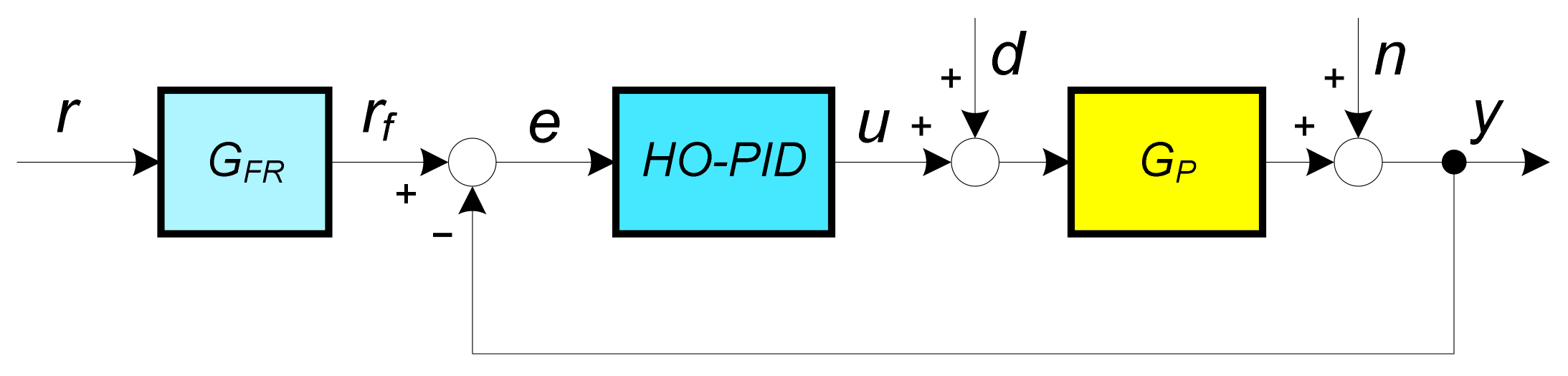
In the paper, the process and the HO-PID controller (1) will be considered, as shown in
Figure 1. Signals
r,
rf,
e,
u,
d,
n and
y stand for the reference, filtered reference, control error, controller output, process input disturbance, process output noise and the process output, respectively. Block
GFR represents the second order filter for the reference signal in order to reduce excessive controller output change on reference changes:
where
TFR denotes the reference filter time constant. Due to simplicity, the filter order in (9) is fixed. However, note that the filter order may be increased by increasing the controller order so as to additionally attenuate the swings of the signal
u for step-like changes of the reference signal
r.
Let us now calculate the process closed-loop transfer function
GCL(
s) from the filtered reference (
rf) to the process output (
y). The closed-loop transfer function is then defined as:
where
Y(
s) and
R(
s) are the Laplace transforms of the process output and the reference signals, respectively.
When applying the process (6) and the controller (1) transfer functions to (10), and considering that the controller binomial filter is a part of the process (in the process transfer function (6) the areas
Ai are replaced by
AiF), the closed-loop transfer function becomes:
where
GOL(s) denotes the open-loop transfer function
GOL(
s) =
GC(
s)
GP(
s).
The MO criteria
According to [
35], the MO tuning criterion states that the closed-loop amplitude (magnitude) should be 1 in as wide a frequency bandwidth as possible (starting from frequency ω = 0). This can be achieved if the open-loop transfer function
GOL(
jω), in the Nyquist diagram, follows the vertical line with the real value −0.5 (according to M and N circles in control theory).
Replacing s with complex frequency
jω in
GOL(
s) (11) yields:
where j denotes the imaginary component
.
Since merely the real part of the open-loop transfer function is required, only the even powers over frequency in (12) are needed. Therefore:
In order to achieve that the
Re{
GOL(
s)} = −0.5 for as high frequencies as possible, the following conditions should be fulfilled:
or in matrix form:
Note that the matrix and vector dimensions depend on the number of controller parameters (
m + 2):
The controller parameters (gains) can then be simply calculated from (15):
The calculation of the controller and filter parameters is straightforward. However, to make it even simpler, we have provided online MATLAB/Octave scripts via the OctaveOnline Bucket website [
39]. The provided scripts calculate all the controller parameters for the given process transfer function and the filter time constant. The website layout is shown in
Figure 2. The calculation procedure proceeds as follows:
Select the appropriate Octave (MATLAB) script (test_HO_TF.m).
Provide the process parameters, the filter time constant, the controller order and filter order,
press the “Save” button, and
press the “Run” button.
The script then calculates the characteristic areas, the controller and the filter parameters. The results are then shown on the right panel of the website.
Illustrative example 1
The
,
and
controller parameters will be calculated for the following processes:
The chosen controller filter time constants is T
F = 0.1. The characteristic areas, without (7), and with controller filter (8) are given in
Table 1.
The calculated controller parameters (17) are given in
Table 2.
In order to reduce the excessive swing of the controller output when changing the reference, the following reference filter time constant (9) is used for both processes:
Note that the second order reference filter is used (9).
The closed-loop responses for the processes
GP1(
s) and
GP2(
s), for all three types of controllers, are shown in
Figure 3 and
Figure 4. It is clear that tracking and control performance increase by the controller order. Note that the controller output response of
controller is not shown entirely in order to see the responses of
and
controllers more clearly.
When comparing process output responses when using controllers
and
in
Figure 3 and
Figure 4, it can be seen that the relative difference in performance is larger on higher-order process
GP1(
s). This is expected, since lower-order processes can already be optimally controlled by lower-order controllers (e.g., the first-order process with
and the second-order process with the
controller). Since the second-order process
GP2(
s) has an additional delay, the closed-loop performance can still be slightly increased with the
controller.
According to the closed-loop responses, it can be concluded that HO-PID controllers can significantly improve the closed-loop performance, especially for higher-order processes. The only required parameter from the user is the controller filter time constant TF. Namely, the amplification of the process output measurement noise depends on the chosen TF. However, the relation between TF and the actual amplification of the high-frequency (HF) noise depends on several other controller parameters and is a rather complex function. Therefore, in practice, it would be more appropriate to define the desired HF noise amplification than the controller filter time constant.
3. HO-PID Controller with Specified HF Noise Amplification
As mentioned in the previous section, the n-th order controller filter GF(s) (1) is primarily used to decrease the controller output noise due to the measurement noise (in addition to making the entire controller transfer function proper or strictly proper and, therefore, realisable in practice). High controller amplification of the measurement noise is never desired, since it may also cause large swings of the control output signals and thus may decrease the actuator’s life span. In order to limit the amplification of the process measurement noise, the user can try different values of TF until the desired amplification (attenuation) of the noise is achieved. In practice, this may take too long, since the function between TF and the noise amplification is complex and non-linear. Therefore, from the user’s perspective, it is easier to define the desired noise amplification of the controller than select filter time constant TF.
The process output noise (
ny) is amplified by the controller (1) in the closed-loop configuration as follows:
where
Ny and
UN are Laplace transforms of the measurement noise and the controller output noise, respectively. The negative sign is omitted to simplify the derivation. From (20) it can be seen that at lower frequencies, the transfer function
GCN(
s) is mostly dominated by the process transfer function
GP(
s), while at higher frequencies, it is mostly dominated by the controller transfer function
GCF(
s). At lower frequencies, the process can be approximated by its gain
KPR, while at higher frequencies the controller gains
K−1 and
K0 can be neglected. Therefore,
GCN(
s) can be approximated by the following transfer function:
On the other hand, the desired controller output noise (
UND) should be similar to:
where
KHF is a chosen noise amplification factor. Since amplitudes
UN and
UND cannot be compared directly due to different frequency characteristics, it is easier to compare noise powers of both signals in some chosen frequency bandwidth (from ω
1 to ω
2). Namely, due to Parseval theorem, the power of the controller output signal (
PUN) is proportional to:
The desired noise power is, according to (22), proportional to:
When considering the
Ny as a white noise with amplitude over frequency as
Ny(
ω) = 1, the powers
PUN and
PUND would become the same when:
However, the solution of the integral in (25), due to the denominator (controller filter), becomes very complex and highly non-linear in respect to TF. Therefore, some search algorithm (optimization) must be applied for each calculation of the TF.
This would seriously impact the simplicity of the proposed method. Therefore, it is decided to simplify the function inside the above integral. Since at higher frequencies, the most dominant controller term becomes the one with the highest derivative (
Km), the function can be simplified as follows:
According to (26), the expression (25) simplifies into:
The contribution of noise power in the frequency region below
ωF is usually much smaller than at higher frequencies. Therefore, in order to even further simplify the derivation, we can choose
ω1 = 0 without making any significant error in the calculation. Selection of the upper frequency (
ω2) in the integral, due to the Shannon theorem, depends on the controller sampling frequency. Without loss of generality, the upper frequency can be selected as:
where
ωS is controller sampling frequency (in rad/s) and
TS is controller sampling time. By taking into account that:
and
ω1 = 0, the expression (27) simplifies even further:
Therefore, the final expression, when taking into account that
Fm =
Km2, reads as:
Therefore, the filter time constant (
TF =1/
ωF) can be estimated as follows:
Note that the above derivation of the filter time constant takes into account approximations (26) and (29). This means that the final output noise power of the controller may differ from that defined by the selected high frequency gain KHF. However, if the above approximations are not taken into account, then the final expressions for the calculation of ωF in (31) would become those of the higher order without analytic solution for TF. This would significantly complicate the filter calculation.
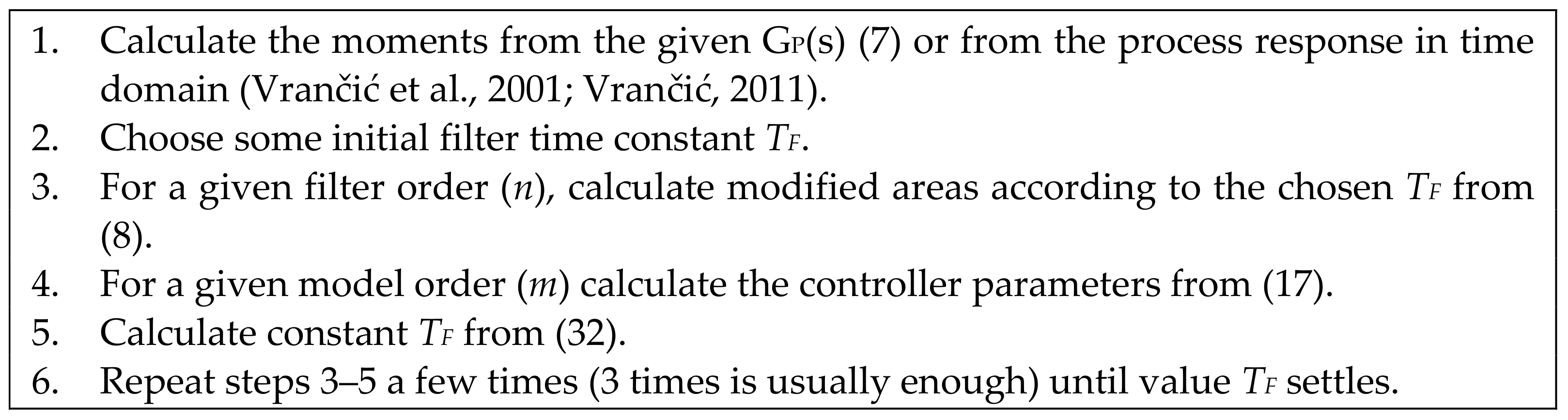
The entire procedure for the calculation of the controller parameters for a given process is given in
Figure 5.
As shown in
Figure 5, the calculation of the controller and filter parameters is straightforward. However, to make it even simpler, as mentioned before, we have provided online MATLAB/Octave scripts via OctaveOnline Bucket website [
39]. The website layout is shown in
Figure 6. The calculation procedure proceeds as follows:
Select the appropriate Octave (MATLAB) script (test_HO_filt.m).
Provide the process parameters, the desired noise gain, the controller sampling time, the controller order and filter order,
press the “Save” button, and
press the “Run” button.
The script then calculates the filter time constant, the characteristic areas and the controller parameters. The results are shown on the right panel of the website.
Illustrative example 2
Consider the following fourth-order process transfer function
GP3(
s) (18):
The initially chosen controller filter time constants is
TF = 0.1. For all the experiments in this section, the chosen sampling time is
TS = 0.002 s. In order to retain clarity of the derivations, the characteristic areas of the process are not mentioned herein; however, they can be calculated (besides all the controller and the filter parameters) on the aforementioned website [
39].
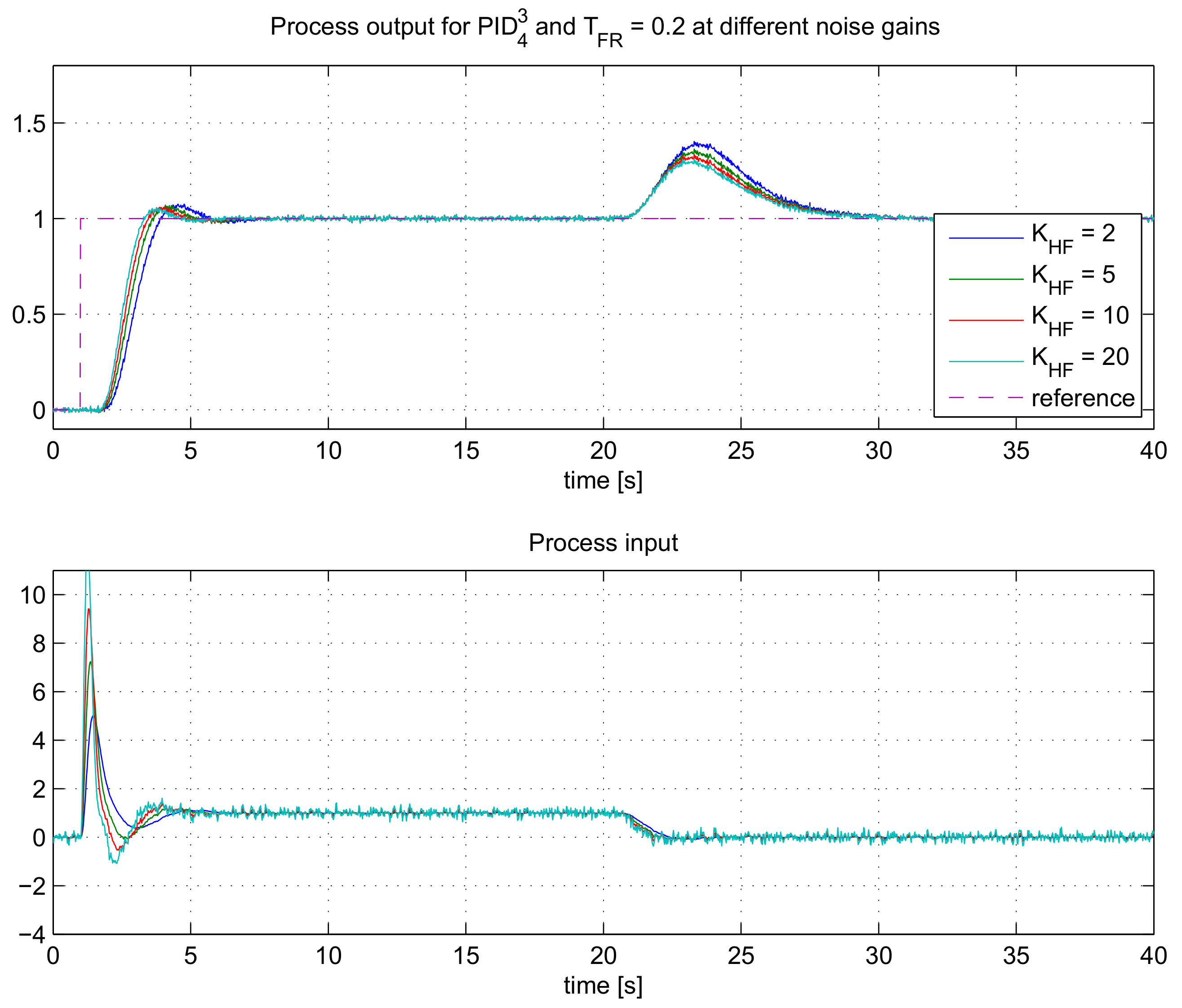
a. Changing the parameter KHF
According to the procedure given in
Figure 5, when choosing parameter
KHF, controller
and repeating steps 3–5 a few times (in our case, 3 times), the calculated filter time constants, and the calculated controller parameters (17) are given in
Table 3.
Again, in order to reduce the excessive swing of the controller output when changing the reference, the following second-order reference filter time constant (9) is used:
The closed-loop responses for different values of
KHF are given in
Figure 7.
As expected, the speed of the closed-loop response and the controller output signal noise increases by increasing the noise gain factor KHF. However, the improvement of the closed-loop speed is not so significant at the highest factors KHF. On the other hand, the controller output noise increases at higher factors KHF. As expected, there is a trade-off between the closed-loop speed and the amount of the controller output noise. Therefore, in practice, the allowed noise gain should be chosen wisely according to the amount of noise present in the system.
The actual “amplification” of the measurement noise (the actually achieved noise gain
KHF) is measured by dividing standard deviations of the controller output signal (
u) and the process output (
n) when the process is in the steady-state:
The actual amplifications of the measurement noise signals are given in
Table 3. It is obvious that the actual gains of the noise (
) are very similar to the desired ones (
KHF).
b. Changing the filter order (n)
On the other hand, the speed of the closed-loop response, for the same KHF and the controller order (m), can also be altered by changing the filter order. In this regard, we tested the performance of the controllers , where n varies from 3 to 6.
According to the procedure given in
Figure 5, when choosing
KHF = 10 and repeating steps 3–5 3 times, the calculated filter time constants and the controller parameters (17) are given in
Table 4.
The closed-loop responses for different controller filter orders (
n = 3 to 6) are given in
Figure 8.
As can be seen, the speed of the closed-loop response is the highest for controller . The speed of controllers with higher-order filters (n > 4) are slightly slower. The speed of response for n > 4 is not improving since a higher-order filter also adds some complexity to the closed-loop transfer function. This, in return, may result in lower closed-loop speeds.
The practical question is how to find the most optimal controller filter order in advance, before making the closed-loop experiment on the process. This can be answered by calculating the integral of control error (
IE), which can be considered as a measure of the closed-loop speed:
If the closed-loop responses have small overshoots, the higher values of IE indicate slower closed-loop responses. For such responses, the IE can be a useful tool to measure the closed-loop speed. The IE value can be relatively easily calculated by transforming the equation (36) into Laplace domain. It can be shown that:
Therefore, for the process with the same steady-state gain
KPR (2), the closed-loop speed is inversely proportional to the integrating gain (
K−1) of the controller. Therefore, the controller with the highest gain
K−1 will produce the fastest closed-loop response (providing that the closed-loop responses have small or negligible overshoots). Indeed, from
Table 4 it is evident that the highest gain
K−1 is calculated for controller
This corresponds to our previous observations.
The actual amplifications of the measurement noise signals, according to (35), are given in
Table 4. The actual noise gains (
) are very similar to the desired ones (
KHF) for filter orders 3 and 4, while for higher-order filters the actual noise gain is lower. This is due to various assumptions (simplifications) made when deriving the filter time constant (32).
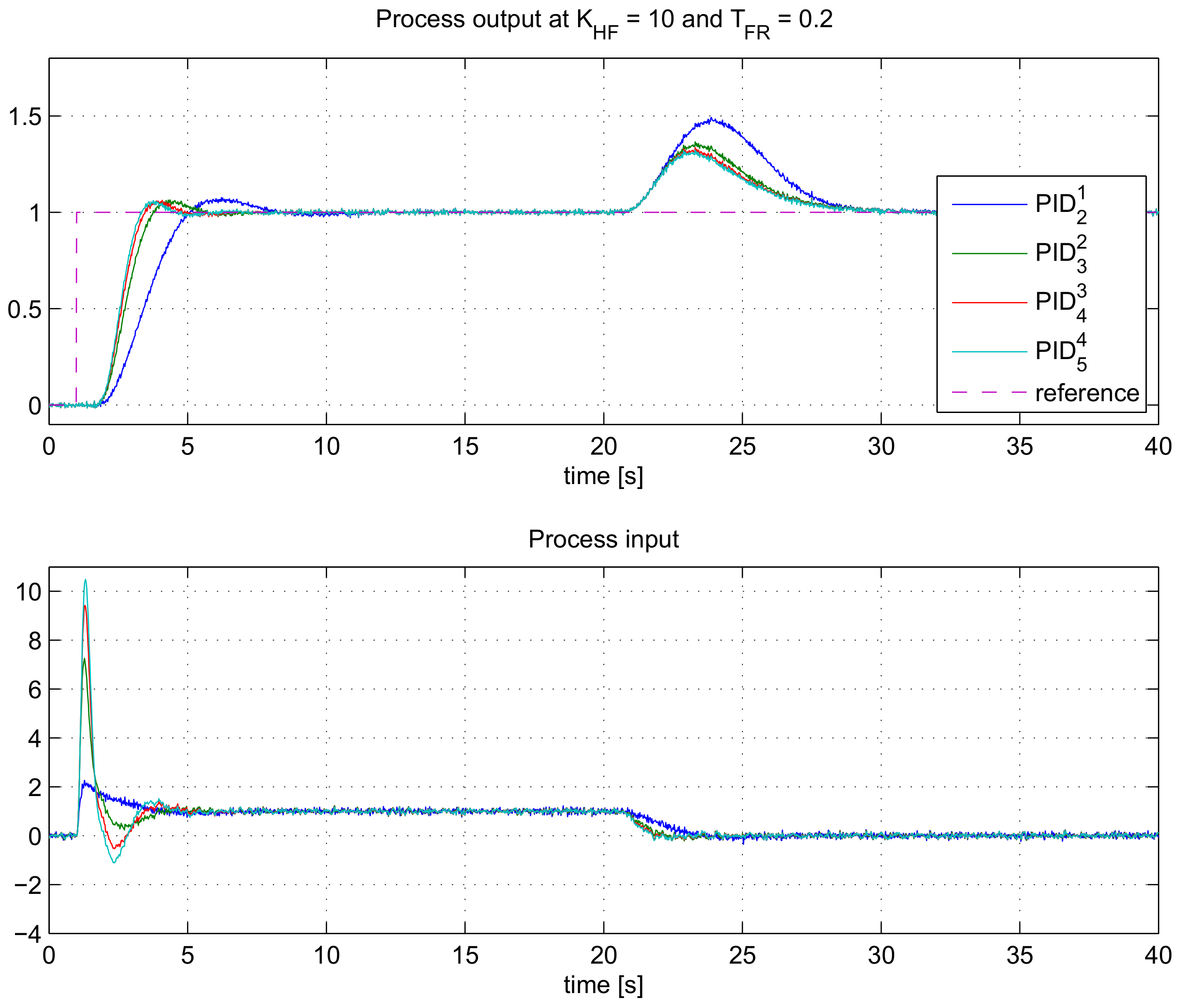
c. Changing the controller order (m)
As is already known, the speed of the closed-loop response can also be altered by changing the controller order. In this regard, we tested the performance of the controllers , where m varies from 1 to 4. In all cases the controller filter is chosen to be 1 order higher than the controller order (n = m + 1). The desired noise gain remains the same as in the previous experiment (KHF = 10).
The calculated filter time constants and the controller parameters (17) are given in
Table 5.
The closed-loop responses for different controller orders (
m = 1 to 4) are given in
Figure 9.
As can be seen, the closed-loop speed increases by increased controller order, similar to the results in
Figure 3 and
Figure 4. The difference is that now the controller output noise is under control (
KHF = 10), so the level of control noise is similar for all of the controllers. The fastest responses are obtained with
. In a similar manner as in the previous case, the speed of responses can be estimated by comparing the values of the calculated integrating gains (
K−1) in
Table 5. Indeed,
K−1 is the highest for
.
The actual amplifications of the measurement noise signals, according to (35), are given in
Table 5. The actual gains of the noise (
) are very similar to the desired ones (
KHF) for all controller orders.
4. Robustness
The proposed design of HO-PID controllers results in a relatively fast and non-oscillatory response. In addition, the controller noise is under control by choosing parameter KHF. However, the designed closed-loop system can still be not robust enough to process variations. Namely, due to nonlinearity or time-variations of the process, its characteristics (gain, delay, time constants, etc.) can vary by working point or by time.
The robustness of a stable closed-loop system is usually measured by maximum sensitivity (
MS) [
1,
38]. Maximum sensitivity is related to the distance of the open-loop transfer function
GC(
jω)
GP(
jω) from the critical point (−1+j0). Namely,
MS is the inverse of the minimum distance between the open-loop transfer function and the critical point. Generally, a smaller value of
MS denotes a more robust closed-loop system to process variations. Usual values of
MS for stable processes are between 1.4 and 2.0 [
1,
38].
The robustness of the closed-loop system for the proposed HO-PID controllers has been tested on the following third-order process with delay:
where the nominal values are
KPR = 1,
Tdel = 1 and
T = 1. Three different HO-PID controllers are selected:
,
, and
. The calculated controller parameters, when choosing
KHF = 10,
TS = 0.002 s and according to the proposed tuning method, are shown in
Table 6. The calculated values of the maximum sensitivity
MS, for all three controllers, are shown in the same table. It can be seen that the
MS values slightly increase with the increased controller order. However, the differences are not large and all the values are below 2.0.
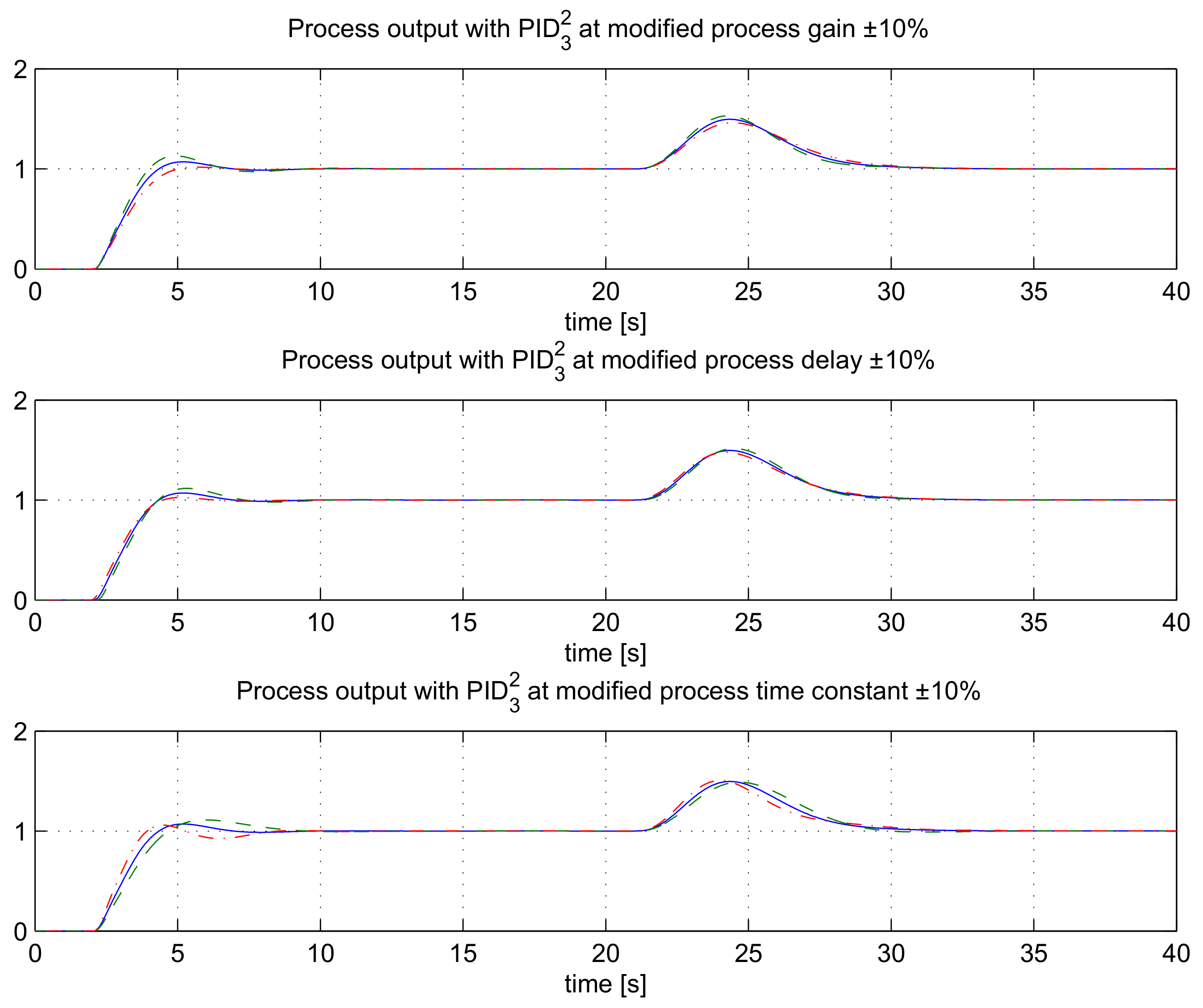
Besides calculating the
MS values, we were also simulating the closed-loop responses using all three controllers on the nominal process, and on the changed process (±10% change of process gain
KPR, time-delay
Tdel and time constant
T). The closed-loop responses are shown in
Figure 10,
Figure 11 and
Figure 12. It is evident that the closed-loop responses under perturbed parameters are still stable without significant oscillations. When comparing
Figure 10 and
Figure 12 it can be noticed that the perturbed parameters with controller
result in slightly more deviation from the nominal response than with controller
. This is all in accordance with the calculated values of
MS in
Table 6.
5. Comparison with Other Tuning Methods
The proposed tuning method was compared with some other methods for PIDA controllers. The chosen methods, which were tested on a particular process model, are from Lurang and Puangdownreong [
21] (denoted as the Lurang method from here on) and Jung and Dorf [
11] (denoted as the Jung method from here on). The Lurang method involves calculating the PIDA controller parameters by optimizing the tracking and disturbance rejection response under several limitations given on rise time, overshoot, settling time, steady-state error and similar. The optimization is carried out with a modified bat algorithm proposed by the authors. The Jung method analytically calculates the PIDA controller parameters for the third-order process according to provided desired overshoot and settling time. Both methods do not take into account the controller’s filter. Therefore, the actual implementation in practice could be questionable if the filter dynamics become slower.
Case 1
The following process model has been selected, according to [
21]:
The Lurang method suggests the following PIDA controller parameters:
The chosen controller filter time constant was very low (TF = 0.01), since we did not want to spoil the closed-loop response of the Lurang method. Namely, as already mentioned, the Lurang method does not take into account the controller filter in the design phase.
For comparison, we chose the controller structures with the lowest possible controller filter order n: . For illustrative purposes, the one-order higher controller structure () was also tested. Note that the closed-loop results of our proposed method, for the same level of controller noise, can be improved by using n > m.
The calculated controller parameters, for the given process and controller filter were the following:
We tested, separately, the tracking response and the disturbance rejection when using all three controllers. For tracking response, the reference (r) changed from 0 to 1 at t = 1 s and for disturbance response the process input disturbance (d) changed from 0 to 1 at t = 1 s.
The closed-loop responses are shown in
Figure 13.
As can be seen, the responses of the proposed method with controller are superior to the Lurang method. Certainly, the one-order higher controller () has a better result.
For a more objective comparison, the integral of squared error (ISE) signal has been calculated for all three controllers. The results are shown in
Table 7. It is obvious that the ISE values for the
controller are much lower than the ones for the Lurang controller.
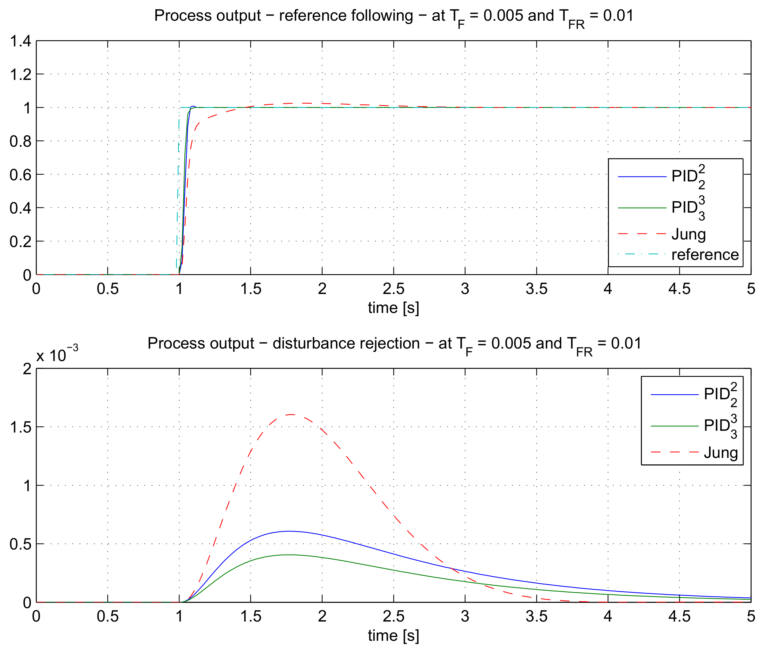
Case 2
The second process model has been selected according to [
11]:
The Jung method suggests the following PIDA controller parameters:
As before, the controller filter time constant was chosen very low (TF = 0.005), since we wanted to preserve the closed-loop response of the Jung method, which was obtained without the controller filter.
The calculated
and
controller parameters, for the given process and controller filter were the following:
As in the previous case, the closed-loop responses were tested on the tracking response and the disturbance rejection. The closed-loop responses are shown in
Figure 14.
Again, the responses of the proposed method with
and
controllers are superior to the Jung method. The comparison of ISE values in
Table 8 shows
controller has lower values than the Jung controller. However, note that the disturbance rejection settling time is the best with the Jung method.
Case 3
The fourth-order process model has been selected according to [
6]:
The Puangdownreong method suggests the following PIDA controller parameters:
The method calculated the following controller filter:
which was also used in design of the proposed
controller parameters. For the given process and controller filter transfer function, the following controller parameters were calculated:
As in the previous case, the closed-loop responses were tested on the tracking response and the disturbance rejection. The closed-loop responses are shown in
Figure 15.
Again, the responses of the proposed method with the
controller are superior to the Puangdownreong method. The comparison of ISE values in
Table 9 shows the
controller has lower values than the Puangdownreong controller.
6. Conclusions
In the paper, the method for tuning the parameters of the m-th order controller with the n-th order binomial filter has been presented. The proposed tuning method is based on the MO criteria which aims to produce non-oscillatory and fast closed-loop reference step responses. The calculation of the controller parameters is analytical and does not require any kind of optimization. An additional advantage of the proposed method is that the process can be described either by the process model or by the process time responses during the steady-state change.
To keep the noise gain of the controller under control, the filter time constant of the controller can also be calculated according to the specified noise gain. The calculation procedure is still analytical, and the results confirm that the level of controller noise is consistent with the given noise gain. The only exception is the use of larger relative degrees between the controller and the filter order, which is the consequence of some simplifications in the calculation of the filter time constant.
The proposed method was tested on six different process models (from second to fourth-order process models with or without time delay). The results confirmed that the control performance can be improved by increasing the controller order or by selecting the filter order appropriately without increasing the controller output noise. The study shows that increasing the filter order improves the performance only up to a certain level, after which the performance starts to decrease. The optimum degree of controller and filter order can be easily determined by the value of integral gain of the controller.
The tuning method was compared with three other tuning methods for PIDA controllers (Lurang [
21], Jung [
11] and Puangdownreong [
6] methods). Although the selected process models were the same as in the aforementioned methods, the proposed method resulted in a better control performance.
Therefore, the proposed higher-order controller design is efficient, and the controller output noise gain is under control. However, it does not mean that the proposed method cannot be improved. Indeed, the proposed method is based on optimizing the reference tracking performance. In our further research, we plan to improve the disturbance rejection performance as well. Namely, the article shows that the MO controller design leads to a strong asymmetry in the dynamics of tracking and disturbance rejection behaviour. While the HO-PID controller design leads to an increase in the number of pulses of the control signal after reference step changes, the responses of the control signal after the change of disturbance remain monotonic. This motivates us to deal with the modification of the MO controller design with regard to a faster response to disturbances.
Moreover, we also plan to design a method that will find the most optimal controller and filter order for the given process and noise amplification considering the complexity of the controller and filter order. We plan to calculate the optimal parameters of the reference filter to control the change of the controller output signal when the reference signal is changed.
Another planned modification is adding a user-defined parameter for changing the speed of the closed-loop control. Slowing down the control speed would further increase the robustness of the system.


