Author Contributions
Conceptualization, L.M.; methodology, L.M.; software, L.M. and J.M.; validation, L.M. and J.M.; investigation, L.M., C.A.M., and J.M.; resources, C.A.M. and C.B.; data curation, L.M. and J.M.; writing—original draft preparation, L.M. and J.M.; writing—review and editing, C.A.M.; supervision, C.A.M. and C.B.; project administration, C.A.M. All authors have read and agreed to the published version of the manuscript.
Figure 1.
Origamipolyhedron Kresling pattern. (a) 2D Kresling pattern. (b) Folded cylinder link state. (c) Biestable behavior.
Figure 1.
Origamipolyhedron Kresling pattern. (a) 2D Kresling pattern. (b) Folded cylinder link state. (c) Biestable behavior.
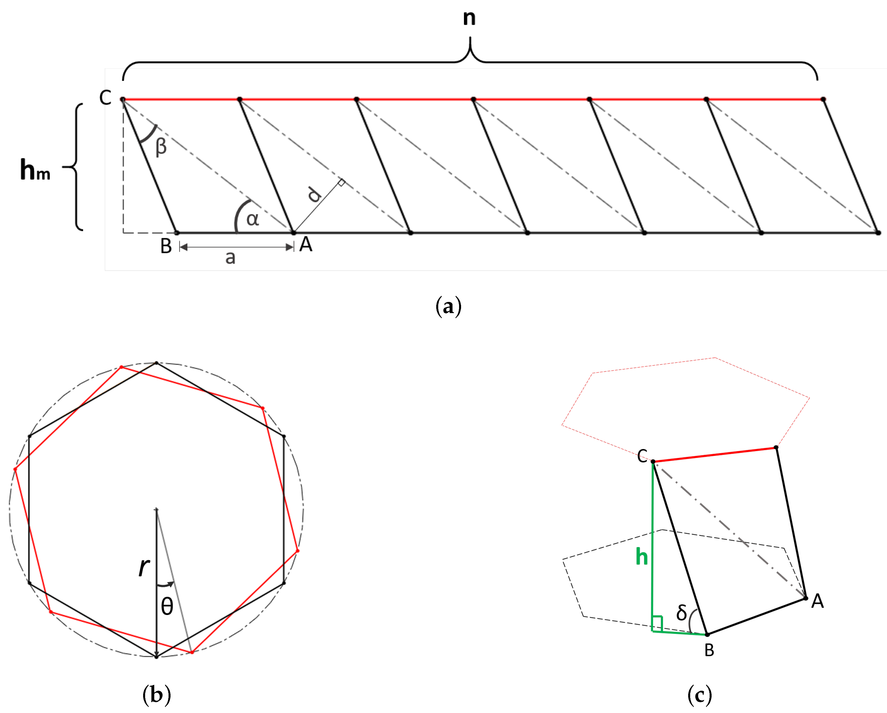
Figure 2.
Cylinder polyhedron origami with one section () and six faces (). (a) Top view collapsed state. (b–d) Folding state.
Figure 2.
Cylinder polyhedron origami with one section () and six faces (). (a) Top view collapsed state. (b–d) Folding state.
Figure 3.
Connection of links. (a) Five-sections link with joints. (b) Joint between links. (c) Joined and reconfigurable links.
Figure 3.
Connection of links. (a) Five-sections link with joints. (b) Joint between links. (c) Joined and reconfigurable links.
Figure 4.
Components of the triangulated polyhedron prototype. (a) Constant base a. (b) Length , greater displacement. (c) Length , minor displacement.
Figure 4.
Components of the triangulated polyhedron prototype. (a) Constant base a. (b) Length , greater displacement. (c) Length , minor displacement.
Figure 5.
Single link CAD prototype. (a) Collapsed state. (b) Folding state. (c) Deployed state.
Figure 5.
Single link CAD prototype. (a) Collapsed state. (b) Folding state. (c) Deployed state.
Figure 6.
Nested links CAD prototype. (a) two-sections link. (b) three-sections link. (c) Two single links with a joint. (d) Two single links with a joint rotated.
Figure 6.
Nested links CAD prototype. (a) two-sections link. (b) three-sections link. (c) Two single links with a joint. (d) Two single links with a joint rotated.
Figure 7.
Single link first prototype. (a) Deployed single link prototype. (b) The single link is in collapsed state, and the height has changed. The pistons are extended and is slightly compressed. (c) Top view of the deployed prototype. (d) Top view of the collapsed prototype; the condition of the pistons and rotation are clearly shown.
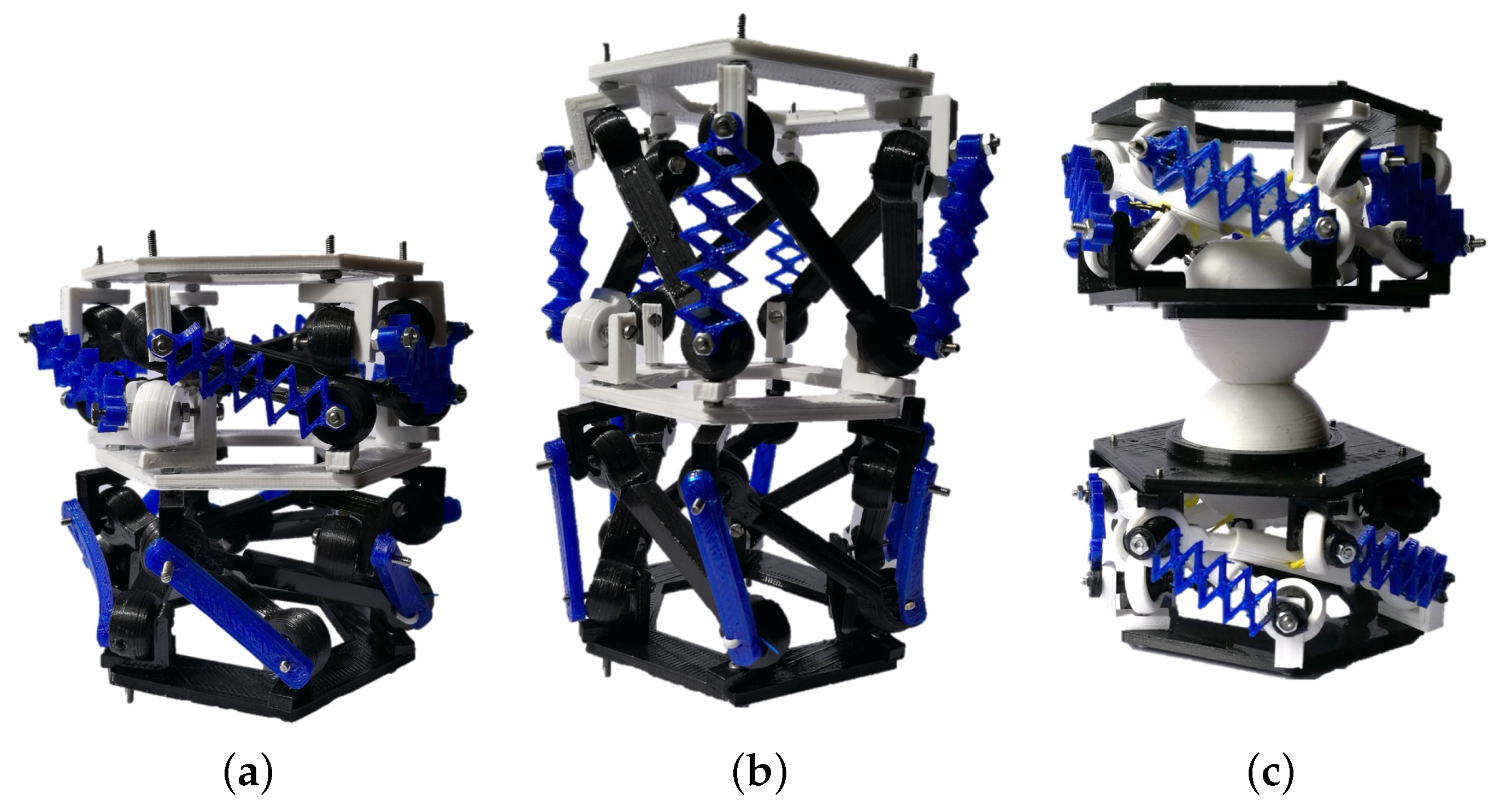
Figure 8.
Assembled nested links prototype. (a) Two-sections link collapsed. (b) Two-sections link deployed. (c) Two single links with a joint. (d) Two single links with a joint, vertically rotated and one of them extended. (e) Two single links with a joint, horizontally rotated and collapsed.
Figure 8.
Assembled nested links prototype. (a) Two-sections link collapsed. (b) Two-sections link deployed. (c) Two single links with a joint. (d) Two single links with a joint, vertically rotated and one of them extended. (e) Two single links with a joint, horizontally rotated and collapsed.
Figure 9.
Cable-driven single link prototype.
Figure 9.
Cable-driven single link prototype.
Figure 10.
Linear regression to obtain the spring elastic constant K from experimental data.
Figure 10.
Linear regression to obtain the spring elastic constant K from experimental data.
Figure 11.
Motor system identification. Different systems identified depending on the inputs (a) and average system time response (b) compared to the captured data.
Figure 11.
Motor system identification. Different systems identified depending on the inputs (a) and average system time response (b) compared to the captured data.
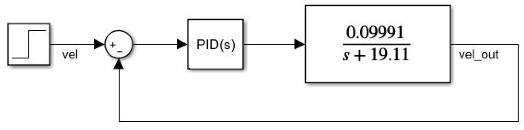
Figure 12.
Motor velocity control system.
Figure 12.
Motor velocity control system.
Figure 13.
Open loop Bode diagram (a) and closed loop time response (b) for the integer order (IOPI) controller.
Figure 13.
Open loop Bode diagram (a) and closed loop time response (b) for the integer order (IOPI) controller.
Figure 14.
Open loop Bode diagram (a) and closed loop time response (b) for the fractional order (FOPI) controller.
Figure 14.
Open loop Bode diagram (a) and closed loop time response (b) for the fractional order (FOPI) controller.
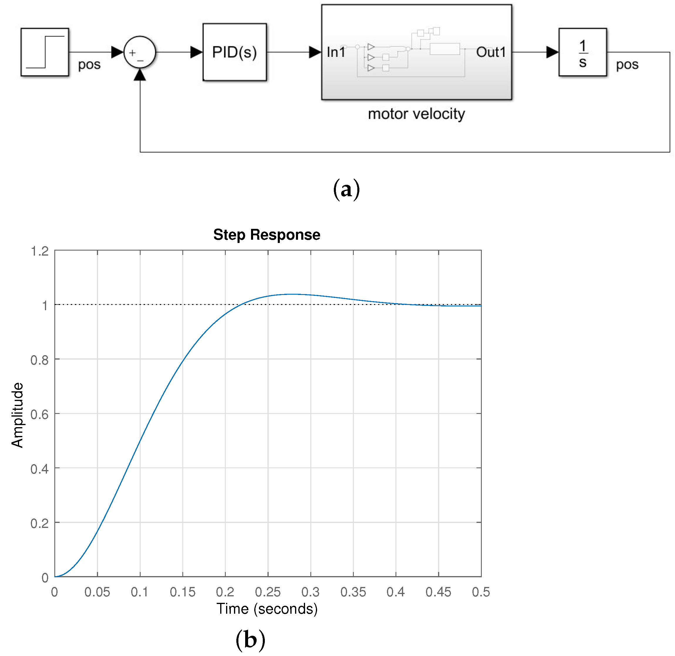
Figure 15.
Motor position control system. Motor position control system. (a) Control system diagram. (b) Step response.
Figure 15.
Motor position control system. Motor position control system. (a) Control system diagram. (b) Step response.
Figure 16.
Origami system identification. Step response in closed loop (a); Bode diagram in open loop (b).
Figure 16.
Origami system identification. Step response in closed loop (a); Bode diagram in open loop (b).
Figure 17.
Origami Kresling single link kinematics vadidation, with parameters , and mm. (a) Collapsed state. (b) Deploying state. (c) Deployed state.
Figure 17.
Origami Kresling single link kinematics vadidation, with parameters , and mm. (a) Collapsed state. (b) Deploying state. (c) Deployed state.
Figure 18.
Three-sections link kinematics validation, with parameters , and mm. (a) Completely deployed link. (b) Only one section folding. (c) Three sections folding.
Figure 18.
Three-sections link kinematics validation, with parameters , and mm. (a) Completely deployed link. (b) Only one section folding. (c) Three sections folding.
Figure 19.
Prototype test results with different target position.
Figure 19.
Prototype test results with different target position.
Figure 20.
Test results with different target positions. (a) Integer controller. (b) Fractional controller.
Figure 20.
Test results with different target positions. (a) Integer controller. (b) Fractional controller.
Figure 21.
Control signals. (a) Position loop control signals with integer controller. (b) Position loop control signals with fractional controller. (c) Velocity loop control signals with Integer controller. (d) Velocity loop control signals with fractional controller.
Figure 21.
Control signals. (a) Position loop control signals with integer controller. (b) Position loop control signals with fractional controller. (c) Velocity loop control signals with Integer controller. (d) Velocity loop control signals with fractional controller.
Figure 22.
Test results with sequential target positions. (a) Integer controller. (b) Fractional controller.
Figure 22.
Test results with sequential target positions. (a) Integer controller. (b) Fractional controller.
Figure 23.
Prototype test results with different payloads in 2.5 (rad) position.
Figure 23.
Prototype test results with different payloads in 2.5 (rad) position.
Figure 24.
Prototype test results with different payloads. (a) Integer controller. (b) Fractional controller.
Figure 24.
Prototype test results with different payloads. (a) Integer controller. (b) Fractional controller.
Figure 25.
Control signals test results with different payloads. (a) Position loop control signals with integer controller. (b) Position loop control signals with fractional controller. (c) Velocity loop control signals with Integer controller. (d) Velocity loop control signals with fractional controller.
Table 1.
Experimental data from spring compression.
Table 1.
Experimental data from spring compression.
| x (m) | M (kg) |
|---|
| 0.13 | 0 |
| 0.128 | 0.1 |
| 0.105 | 0.2 |
| 0.092 | 0.3 |
| 0.082 | 0.4 |
Table 2.
Equivalence between frequency specifications and time response.
Table 2.
Equivalence between frequency specifications and time response.
| Physical | Effect | Closed Loop | Open Loop |
|---|
| Meaning | Defined | Specification | Specification |
|---|
| Damping ratio | Overshoot | Resonant peak | Phase margin |
| Response speed | Peak time | Bandwidth | Crossover frequency |
Table 3.
Data from single link kinematics simulation.
Table 3.
Data from single link kinematics simulation.
| | h (mm) | (deg) | (deg) |
|---|
| Collapsed state | 0 | 0 | −13.32 |
| Deploying state | 30 | 54.3 | −12.27 |
| Deployed state | 36.93 | 90 | 1.04 |
Table 4.
Three-sections link kinematics simulation data.
Table 4.
Three-sections link kinematics simulation data.
| | (mm) | (mm) | (mm) | (mm) |
|---|
| Completely deployed link | 36.93 | 36.93 | 36.93 | 110.8 |
| Only one section folding | 36.93 | 20.55 | 36.93 | 94.43 |
| Three sections folding | 31.73 | 25.55 | 30 | 87.29 |
Table 5.
Experimental kinematic data indirectly computed.
Table 5.
Experimental kinematic data indirectly computed.
| Real | Simulation | Error |
|---|
| Position (rad) | h (mm) | (deg) | (deg) | h (mm) | (deg) | h (mm) | (deg) |
| 0.5 | 35.69 | 64.46 | −12.11 | 38.88 | −12.28 | 3.18 | −0.1635 |
| 1 | 31.94 | 53.85 | −12.72 | 34.79 | −12.89 | 2.84 | −0.1637 |
| 1.5 | 28.19 | 45.45 | −13.06 | 30.71 | −13.23 | 2.51 | −0.1660 |
| 2 | 24.44 | 38.16 | −13.28 | 26.64 | −13.45 | 2.19 | −0.1634 |
| 2.2 | 22.94 | 35.45 | −13.35 | 24.99 | −13.52 | 2.04 | −0.1642 |


