Geometrical Properties of the Pseudonull Hypersurfaces in Semi-Euclidean 4-Space

Abstract

In this paper, we focus on some geometrical properties of the partially null slant helices in semi-Euclidean 4-space. By structuring suitable height functions, we obtain the singularity types of the pseudonull hypersurfaces, which are generated by the partially null slant helices. An example is given to determine the main results.

1. Introduction

Since Einstein put forward the theory of relativity in 1915, semi-Euclidean space has attracted the attention of many geometry and physics scholars. Compared with Euclidean space, the characteristic of semi-Euclidean space is the existence of a lightlike vector. There are three types of curves (surfaces) in semi-Euclidean space: spacelike curves (surfaces), timelike curves (surfaces), and lightlike curves (surfaces) [1,2,3,4]. In physics, Hiscock WA [5] obtained that the horizon of the black hole was a null hypersurface. In this paper, we construct a special kind of null hypersurface along a partially null slant helix and obtain its singularity types, which can help scientists to further study the shape of the black hole horizon.

There are many examples and phenomena of helical structures in nature, such as carbon nanotubes and the DNA double helical structure, among others. Amand AL and Lambin P [6] stated that the DNA double helical structure was believed to be one of the most important subjects in biology. Izumiya S and Takeuchi N [7] gave the definition of the slant helix in Euclidean space. Abazari N [8] obtained the stationary acceleration in Minkowski space. Yaliniz AF, Hacisalihoglu HH [9] obtained some geometry properties of the null generalized helices in ${\mathbb{L}}^{m+2}$. The third author and Hou [10] gave a new kind of helicoidal surface in Minkowski 3-space. Mosa S, Elzawy M [11] considered the differential geometrical properties of the helicoidal surfaces in Galilean 3-space.

Petrović-Torgašev M, Ilarslan K, and Nešović E [12] gave definitions and some geometrical properties of partially null curves and pseudonull curves in ${\mathbb{R}}_2^4$; Ali A, López R, and Turgut M [13] defined the k-type partially null and pseudonull slant helices in ${\mathbb{R}}_1^4$. Harslan K and Nešović E [14] obtained the geometrical properties of the null helices and gave some characterizations for the timelike and null helices. We find that many papers about the helical curves only considered the smooth properties, but few considered the singular properties. Therefore, starting from the singularity, in this paper, we study the singularity properties of the pseudonull hypersurfaces of the partially null slant helices in semi-Euclidean 4-space with index two using singularity theory.

In the research of geometric properties of submanifolds, singularity is an inevitable research object. Singularity is widely used in many disciplines, such as biology and physics, among others. The singularities of surfaces and curves in Euclidean space or semi-Euclidean space were studied in [4,15,16,17,18,19]. The first author [1,20] studied the singularity properties of some null curves in different spaces. In this paper, we investigate the differential geometry and the singularity properties of the pseudonull hypersurfaces of the partially null slant helices in semi-Euclidean 4-space.

We organize the present manuscript as follows. In the second section, we introduce the definition of the pseudonull hypersurface and obtains some geometrical properties of the partially null slant helices. Meanwhile, the main singularity result (the Theorem 3) is also given in this section. The height functions of partially null slant helices are constructed to describe the contract relation in Section 3. For the remainder of this paper, we consider the versal unfolding and the generic properties of the partially null slant helices to prove Theorem 3 in Section 4. In the last section, we give one example to insist on our results.

2. Preliminaries and the Main Results

Let $\mathit{\gamma }:I\subset \mathbb{R}\to {\mathbb{R}}_2^4$ be an arc-length parameterized differentiable curve with Frenet frames $\mathit{T}(s),$ $\mathit{N}(s),$ ${\mathit{B}}_1(s),$ and ${\mathit{B}}_2(s)$, where $\mathit{T}(s)$ is called the tangent vector, $\mathit{N}(s)$ is called the principal normal vector, ${\mathit{B}}_1(s)$ is called the first binormal vector, and ${\mathit{B}}_2(s)$ is called the second binormal vector [13].

For a fixed constant vector field $\mathit{U}$, we call $\mathit{\gamma }(s)$ a 0-type, 1-type, 2-type, or 3-type slant helix if and only if $\langle \mathit{T}(s),\mathit{U}\rangle =c,$ $\langle \mathit{N}(s),\mathit{U}\rangle =c,$ $\langle {\mathit{B}}_1(s),\mathit{U}\rangle =c,$ or $\langle {\mathit{B}}_2(s),\mathit{U}\rangle =c,$ respectively, where c is a constant.

First, the definition of a partially null curve is given by the following [12,13].

Definition 1. 

Let $\mathit{\gamma }(s)$ be an arc-length parameterized differentiable curve with Frenet frames $\{\mathit{T}(s),$ $\mathit{N}(s),$ ${\mathit{B}}_1(s),$ ${\mathit{B}}_2(s)\}$, satisfying the following conditions:

$$\langle \mathit{T}(s),\mathit{T}(s)\rangle =-\langle \mathit{N}(s),\mathit{N}(s)\rangle =-\epsilon ,\epsilon =\pm 1,$$

$$\langle {\mathit{B}}_1(s),{\mathit{B}}_1(s)\rangle =\langle {\mathit{B}}_2(s),{\mathit{B}}_2(s)\rangle =0,\langle {\mathit{B}}_1(s),{\mathit{B}}_2(s)\rangle =1,$$

$$\langle \mathit{T}(s),\mathit{N}(s)\rangle =\langle \mathit{T}(s),{\mathit{B}}_1(s)\rangle =\langle \mathit{N}(s),{\mathit{B}}_1(s)\rangle =0,$$

$$\langle \mathit{T}(s),{\mathit{B}}_2(s)\rangle =\langle \mathit{N}(s),{\mathit{B}}_2(s)\rangle =0.$$

We call the curve $\mathit{\gamma }(s)$ a partially null curve.

The Frenet formulas of the partially null curve are given by the following equations [13]:

$$\begin{array}{c}\hfill \left\{\begin{array}{c}{\mathit{T}}^{\prime }(s)=k_1(s)\mathit{N}(s)\hfill \\ {\mathit{N}}^{\prime }(s)=k_1(s)\mathit{T}(s)+k_2(s){\mathit{B}}_1(s)\hfill \\ {\mathit{B}}_1^{\prime }(s)=k_3(s){\mathit{B}}_1(s)\hfill \\ {\mathit{B}}_2^{\prime }(s)=-\epsilon k_2(s)\mathit{N}(s)+k_3(s){\mathit{B}}_2(s)\hfill \end{array}\right.,\end{array}$$

(1)

where $k_1(s)=\epsilon \langle {\mathit{T}}^{\prime }(s),\mathit{N}(s)\rangle$, $k_2(s)=\langle N^{\prime }(s),{\mathit{B}}_2(s)\rangle ,$ and $k_3(s)=\langle {\mathit{B}}_1^{\prime }(s),{\mathit{B}}_2(s)\rangle$ are called the curvature functions of the partially null curve $\mathit{\gamma }(s).$ We call a curve a 0-type partially null slant helix if the curve is a partially null curve with $\langle \mathit{T}(s),\mathit{U}\rangle =constant.$ When $k_1(s)k_2(s)=0,$ we have the following remark.

Remark 1. 

When $k_1(s)=0(k_2(s)=0)$, from Equations (1), we can ascertain that $\mathit{T}(s)$ $({\mathit{B}}_2(s))$ is a constant vector and the rectifying space at every points of $\mathit{\gamma }(s)$ are parallel. So $\mathit{\gamma }(s)\subset HP(T(s),0)\subset {\mathbb{R}}_1^3(\mathit{\gamma }(s)\subset HP({\mathit{B}}_2(s),0)\subset {\mathbb{R}}_1^3)$ or $\mathit{\gamma }(s)\subset {\mathbb{R}}_2^3$. The two spaces ${\mathbb{R}}_1^3,{\mathbb{R}}_2^3$ are equal. In the following text, we only consider $k_1(s)k_2(s)\ne 0$.

Theorem 1. 

Let $\mathit{\gamma }(s)$ be a 0-type partially null slant helix in ${\mathbb{R}}_2^4$ if and only if $k_1(s)/k_2(s)$ is constant for any $s\in I$.

Proof. 

Let $\mathit{\gamma }(s)$ be a 0-type partially null slant helix, we choose a constant vector $\mathit{U}$ satisfying

$$\langle \mathit{T}(s),\mathit{U}\rangle =c,$$

(2)

where c is constant. By taking the derivative of the Equation (2) with respect to s, we assume there exist two coefficients $u_3$ and $u_4$, the constant vector $\mathit{U}$ can be written easily:

$$\mathit{U}=c\mathit{T}(s)+u_3{\mathit{B}}_1(s)+u_4{\mathit{B}}_2(s).$$

(3)

Differentiating the both sides of the Equation (3), we can find the following equations:

$$\begin{array}{c}\hfill \left\{\begin{array}{c}{u}_4^{\prime }=0\hfill \\ -\epsilon c{k}_1(s)-\epsilon k_2(s)u_4=0\hfill \end{array}\right..\end{array}$$

(4)

Hence, we obtain that $k_1(s)/k_2(s)$ is a constant with $k_2(s)\ne 0$. The contrary is clearly established. We completed the proof. □

Theorem 2. 

In ${\mathbb{R}}_2^4,$ $\mathit{\gamma }(s)$ is a 0-type partially null slant helix; then, $\mathit{\gamma }(s)$ is also a 1-type, 2-type, or 3-type partially null slant helix.

Proof. 

Let $\mathit{\gamma }(s)$ be a 0-type partially null slant helix. From the Theorem 1, we can obtain the following conclusion:

$$k_1(s)\langle \mathit{N}(s),\mathit{U}\rangle =0.$$

(5)

Hence $\mathit{\gamma }(s)$ is a 1-type partially null slant helix. Taking the derivative from both sides of the Equation (5) with respect to s and using Frenet Equation (1), we obtain the following statements:

$$k_1(s)\langle \mathit{T}(s),\mathit{U}\rangle +k_2(s)\langle {\mathit{B}}_1(s),\mathit{U}\rangle =0,$$

(6)

and

$$\langle {\mathit{B}}_1(s),\mathit{U}\rangle =-c{k}_1(s)/k_2(s)=-c{c}^{\prime }=constant.$$

(7)

Hence, $\mathit{\gamma }(s)$ is also a 2-type partially null slant helix. Similarly,

$${\langle {\mathit{B}}_2(s),\mathit{U}\rangle }^{\prime }=\langle {\mathit{B}}_2^{\prime }(s),\mathit{U}\rangle =-\epsilon k_2(s)\langle -\mathit{N}(s),\mathit{U}\rangle =0.$$

(8)

We know $\langle {\mathit{B}}_2(s),\mathit{U}\rangle$ is constant, and $\mathit{\gamma }(s)$ is a 3-type partially null slant helix. □

As the same method of the Theorem 2, we have the following conclusion:

Corollary 1. 

In ${\mathbb{R}}_2^4,$ $\mathit{\gamma }(s)$ is a 1-type partially null slant helix if and only if $\mathit{\gamma }(s)$ is a 3-type partially null slant helix.

Let $\mathit{\gamma }(s)$ be a 0-type partially null slant helix in ${\mathbb{R}}_2^4$. We define a surface with the base curve $\mathit{\gamma }(s)$ as following:

$$\mathcal{PNH}(s,\lambda ,\eta )=\mathit{\gamma }(s)-\lambda T(s)-\eta B_2(s),$$

$$BC({\mathit{v}}_0)=\{u\in {\mathbb{R}}_2^4\mid \langle u-{\mathit{v}}_0,B_2(s)\rangle =0\},$$

we call $\mathcal{PNH}(s,\lambda ,\eta )$ the pseudonull hypersurface of $\mathit{\gamma }(s)$, which is a ruled hypersurface. We call $BC({\mathit{v}}_0)$ the hyperplane.

We can obtain the main result of the singularity types of the pseudonull hypersurface $\mathcal{PNH}$ by the following theorem.

Theorem 3. 

Let $\mathit{\gamma }(s)$ be a 0-type partially null slant helix; for ${\mathit{v}}_0=\mathcal{PNH}(s_0,{\lambda }_0,{\eta }_0)$, we have the following:

(1) 

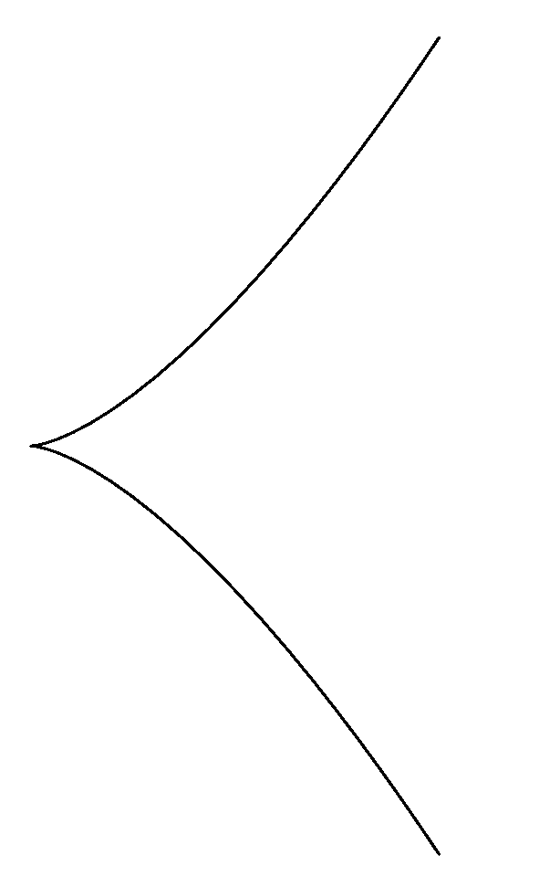
$\mathit{\gamma }(s)$ and $BC({\mathit{v}}_0)$ have at least 2-point contact at $s_0$ (Figure 1).

(2) 

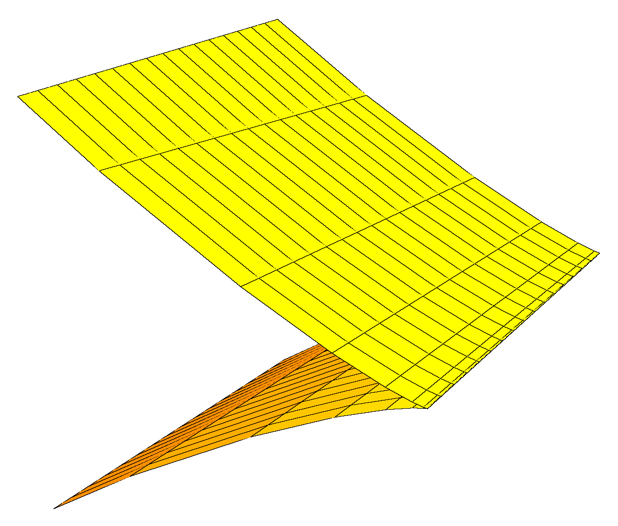
$\mathit{\gamma }(s)$ and $BC({\mathit{v}}_0)$ have 3-point contact at $s_0$ if and only if ${\mathit{v}}_0=\mathit{\gamma }(s)-\eta (\epsilon (k_2(s)/k_1(s))\mathit{T}(s)$ $+{\mathit{B}}_2(s)),\eta \ne 1$, under this condition, the germ of ${\mathit{v}}_0$ is diffeomorphism to the cuspidal edge (Figure 2).

(3) 

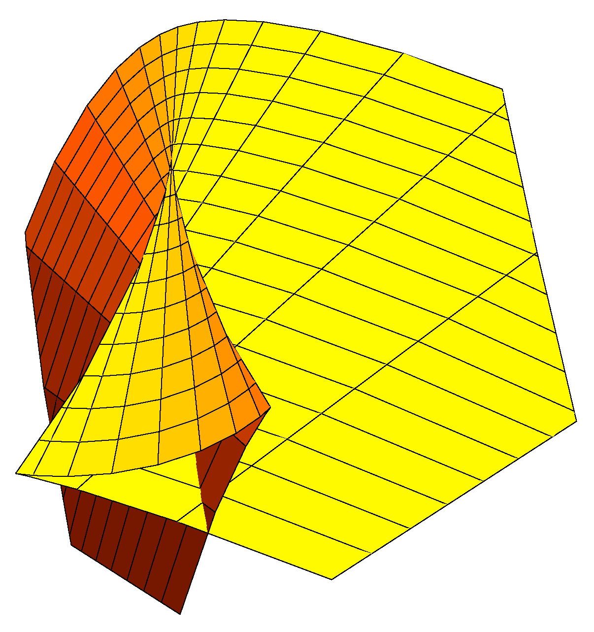
$\mathit{\gamma }(s)$ and $BC({\mathit{v}}_0)$ have 3-point contact at $s_0$ if and only if ${\mathit{v}}_0=\mathit{\gamma }(s)-\eta (\epsilon (k_2(s)/k_1(s))$ $\mathit{T}(s)+{\mathit{B}}_2(s)),\eta =1$, under this condition, the germ of ${\mathit{v}}_0$ is diffeomorphism to the swallowtail (Figure 3).

Here $C\times \mathbb{R}=\{(x_1,x_2,x_3)\mid x_1=u,x_2=\pm v^{1/2},x_3=v^{1/3}\}$ is the cuspidal edge and $SW=\{(x_1,x_2,x_3)\mid x_1=3u^4+u^{2}v,x_2=4u^3+2uv,x_3=v\}$ is the swallowtail.

3. The Height Function

In this section, we mainly give the definition of the height function on $\mathit{\gamma }(s)$ to describe the contact relationship.

Let $\mathit{\gamma }(s)$ be a 0-type partially null slant helix in ${\mathbb{R}}_2^4$. The height function $H:I\times {\mathbb{R}}_2^4\to \mathbb{R}$ is given as

$$H(s,\mathit{v})=\langle \mathit{\gamma }(s)-\mathit{v},{\mathit{B}}_2(s)\rangle .$$

We write $h_v(s)=H(s,\mathit{v})$ for any fixed vector $\mathit{v}$. Then, we have the following proposition:

Proposition 1. 

Let $\mathit{\gamma }(s)$ be a 0-type partially null slant helix in ${\mathbb{R}}_2^4$, for a fixed vector $\mathit{v}\in {\mathbb{R}}_2^4.$ Then, we have

(1)

$h_v(s)=0$ if and only if there exist three real numbers $\lambda ,\omega ,\eta$, such that $\mathit{\gamma }(s)-\mathit{v}=\lambda \mathit{T}(s)+\omega \mathit{N}(s)+\eta {\mathit{B}}_2(s)$.

(2)

$h_v(s)=h_v^{\prime }(s)=0$ if and only if $\mathit{v}=\mathit{\gamma }(s)-\lambda \mathit{T}(s)-\eta {\mathit{B}}_2(s)$.

(3)

$h_v(s)=h_v^{\prime }(s)=h_v^{″}(s)=0$ if and only if $\mathit{v}=\mathit{\gamma }(s)-\eta (\epsilon (k_2(s)/k_1(s))\mathit{T}(s)+{\mathit{B}}_2(s)),$ $\eta \ne 1$.

(4)

$h_v(s)=h_v^{\prime }(s)=h_v^{″}(s)=h_v^{‴}(s)=0$ if and only if $\mathit{v}=\mathit{\gamma }(s)-\eta (\epsilon (k_2(s)/k_1(s))\mathit{T}(s)+{\mathit{B}}_2(s)),\eta =1$.

Proof. 

(1). Let us assume that $\mathit{v}=\lambda \mathit{T}(s)+\omega \mathit{N}(s)+\xi {\mathit{B}}_1(s)+\eta {\mathit{B}}_2(s),$ where $\lambda ,\omega ,\xi ,\eta \in \mathbb{R}$. Thus, it can be seen that $h_v(s)=0$ if and only if $\xi =0,$ we obtain the statement (1).

(2). Differentiating both sides of the Equation $h_v(s)=0$ with respect to s and using Frenet Equation (1), we get

$$\begin{array}{cc}{h}_v^{\prime }(s)\hfill & =\langle {\mathit{\gamma }}^{\prime }(s),{\mathit{B}}_2(s)\rangle +\langle \mathit{\gamma }(s)-\mathit{v},{\mathit{B}}_2^{\prime }(s)\rangle \hfill \\ \hfill & =\langle {\mathit{\gamma }}^{\prime }(s),{\mathit{B}}_2(s)\rangle +\langle \mathit{\gamma }(s)-\mathit{v},-\epsilon k_2(s)\mathit{N}(s)\rangle \hfill \\ \hfill & =k_2(s)\omega ,\hfill \end{array}$$

(9)

and in the view of $k_2(s)\ne 0$, it can be seen that $\omega =0$. The statement (2) is supported.

(3). Similarly, differentiating both sides of the Equation (9) with respect to s and using Frenet Equation (1),

$$\begin{array}{cc}{h}_v^{″}(s)\hfill & =\langle {\mathit{\gamma }}^{\prime }(s),-\epsilon k_2(s)\mathit{N}(s)\rangle +\langle \mathit{\gamma }(s)-\mathit{v},-\epsilon k_2^{\prime }(s)\mathit{N}(s)-k_2(s){\mathit{N}}^{\prime }(s)\rangle \hfill \\ \hfill & =\langle \mathit{\gamma }(s)-\mathit{v},-\epsilon k_2^{\prime }(s)\mathit{N}(s)-\epsilon k_2(s)(k_1(s)\mathit{T}(s)+k_2(s){\mathit{B}}_1(s))\rangle ,\hfill \\ \hfill & =\lambda k_1(s)k_2(s)-\epsilon \eta k_2^2(s).\hfill \end{array}$$

(10)

It can be seen that $\lambda /\eta =\epsilon (k_2(s)/k_1(s))$. We obtain the statement (3).

(4). Taking the derivative of the Equation (10) with respect to s and using Frenet Equation (1), we can obtain

$$\begin{array}{cc}{h}_v^{‴}(s)\hfill & =\langle {\mathit{\gamma }}^{\prime }(s),-\epsilon k_2^{\prime }(s)\mathit{N}(s)-\epsilon k_2(s){\mathit{N}}^{\prime }(s)\rangle \hfill \\ \hfill & +\langle \mathit{\gamma }(s)-\mathit{v},-\epsilon k_2(s){(k_1(s)\mathit{T}(s)+k_2(s){\mathit{B}}_1(s))}^{\prime }\rangle \hfill \\ \hfill & =k_1(s)k_2(s)+\langle \mathit{\gamma }(s)-\mathit{v},-\epsilon (k_1(s)k_2^{\prime }(s)+{(k_1(s)k_2(s))}^{\prime }\hfill \\ \hfill & -(2k_2^{″}(s)+\epsilon k_1^2(s)k_2(s)))\mathit{T}(s)+(k_1(s)+k_2^{″}(s))\mathit{N}(s)+2\epsilon (k_1^{\prime }(s)k_2(s)){\mathit{B}}_1(s)\rangle \hfill \\ \hfill & =k_1(s)k_2(s)+\lambda (k_1(s)k_2(s)+{(k_1(s)k_2(s))}^{\prime }-2k_1^{\prime }(s)k_2(s)).\hfill \end{array}$$

(11)

Thus, $\lambda =k_1(s)k_2(s)/(k_1(s)k_2(s)+{(k_1(s)k_2(s))}^{\prime }-2k_1^{\prime }(s)k_2(s))=1$ when $h_v^{‴}(s)=0$. □

4. The Proof of the Theorem 3

In this section, we use some general results on the singularity theory [15] to prove the main result (Theorem 3).

Firstly, we introduce two important sets. The singular set of F is the set

$${\mathfrak{S}}_F=\{(s,x)\in \mathbb{R}\times {\mathbb{R}}^r|\partial F/\partial s(s,x)=0\}.$$

The discriminant set of F is the set

$${\mathfrak{D}}_F=\{x\in {\mathbb{R}}^r|\mathrm{there}\mathrm{exists}s\mathrm{with} F=\partial F/\partial s=0at(s,x)\}.$$

Then, applying the main result of Theorem 4.1 in [16] and the versal unfolding in [18], for the height function H of the 0-type partially null slant helix, we obtain the following theorem:

Theorem 4. 

Let $\mathit{\gamma }(s)$ be a 0-type partially null slant helix and ${\mathit{v}}_0\in {\mathfrak{D}}_H$, H is a versal unfolding of $h_{v_0}$ if $h_{v_0}$ has $A_k$-singularity at $s(k=1,2)$.

Proof. 

Suppose $\mathit{\gamma }(s)=(x_1(s),x_2(s),x_3(s),x_4(s)),$ $\mathit{v}(s)=(v_1(s),v_2(s),v_3(s),v_4(s)),$ and ${\mathit{B}}_1(s)=\{b_1(s),b_2(s),b_3(s),b_4(s)\}.$

We have $H(s,\mathit{v})=-(x_1(s)-v_1(s))b_1(s)-(x_2(s)-v_2(s))b_2(s)+(x_3(s)-v_2(s))b_3(s)$ $+(x_4(s)-v_4(s))b_4(s),$

$$\partial H/\partial v_i=b_i(s)i=1,2;\partial H/\partial v_j=-b_j(s),j=3,4$$

$${\partial }^{2}H/\partial s\partial v_i=b_i^{\prime }(s),i=1,2;{\partial }^{2}H/\partial s\partial v_j=-b_j^{\prime }(s),j=3,4$$

and

$${\partial }^{3}H/{\partial }^{2}s\partial v_i=b_i^{″}(s),i=1,2;{\partial }^{3}H/{\partial }^{2}s\partial v_j=-b_j^{″}(s).j=3,4$$

Let $j^2\partial H/\partial v_i(s,v_0)(s_0)$ be the 2-jet of $\partial H/\partial v_i(s,v)(i=1,2,3,4)$ at $s_0$, we can show that

$$\partial H/\partial v_i(s_0,v_0)+j^2\partial H/\partial v_i(s,v_0)(s_0)={\alpha }_{0,i}+{\alpha }_{1,i}(s-s_0)+1/2{\alpha }_{2,i}{(s-s_0)}^2,$$

(12)

where $\partial H/\partial v_i(s_0,v_0)={\alpha }_{0,i},$ ${\partial }^{2}H/\partial s\partial v_i(s_0,v_0)(s-s_0)={\alpha }_{1,i},$ and

$${\partial }^{3}H/{\partial }^{2}s\partial v_i(s_0,v_0){(s-s_0)}^2={\alpha }_{2,i}.$$

We denote that

$$\mathcal{M}=\left(\begin{array}{c}{\alpha }_{0,1}{\alpha }_{0,2}{\alpha }_{0,3}{\alpha }_{0,4}\end{array}\right),\mathcal{Z}=\left(\begin{array}{c}{\alpha }_{0,1}{\alpha }_{0,2}{\alpha }_{0,3}{\alpha }_{0,4}\\ {\alpha }_{1,1}{\alpha }_{1,2}{\alpha }_{1,3}{\alpha }_{1,4}\end{array}\right).$$

When h has $A_1$-singularity at $s_0$, by the Proposition 1, there exist two nonzero numbers $\lambda ,\eta$ satisfying

$$h(s_0)-\mathit{v}=\eta (\epsilon (k_2(s)/k_1(s))\mathit{T}(s)+{\mathit{B}}_2(s)).$$

We can see that the rank of $\mathcal{M}$ is 1 since ${\mathit{B}}_2(s)\ne \mathbf{0}.$ From the Proposition 1, h has $A_2$-singularity at $s_0$ if and only if $h(s_0)-\mathit{v}=\eta (\epsilon (k_2(s)/k_1(s))\mathit{N}(s)+{\mathit{B}}_2(s))$, $\eta \ne \epsilon$. When h has $A_2$-singularity at $s_0,$ we require the rank of $\mathcal{Z}$ is 2.

$$\begin{array}{cc}det\mathcal{Z}\hfill & =det({\mathit{B}}_2(s_0),{\mathit{B}}_2^{\prime }(s_0),{\mathit{B}}_2^{″}(s_0))\ne 0\hfill \end{array}$$

(13)

This completes the proof. □

Then, we have the following proposition as a corollary of Lemma 6 [16].

Proposition 2. 

Let $\mathcal{O}$ be a submanifold of $J^l(1,1).$ Then the set $T_{\mathcal{O}}=\{\mathit{\gamma }(s)\in Em{b}_s(I,{\mathbb{R}}_2^4)\mid j_1^l(H)$ is transversal to $\mathcal{O}\}$ is a residual subset of $Emb(I,{\mathbb{R}}_2^4).$ If $\mathcal{O}$ is a closed subset, then $T_{\mathcal{O}}$ is open.

There is another characterization of the versal unfolding as follows [15],

Proposition 3. 

Let $F:(\mathbb{R}\times {\mathbb{R}}^r,\mathbf{0})\to (\mathbb{R},0)$ be an r-parameter unfolding of $f:(\mathbb{R},0)\to (\mathbb{R},0),$ which has $A_k$-singularity at 0. Then, F is a versal unfolding if and only if $j_1^{l}F$ is transversal to the orbit $L^l\widetilde{(j^{l}f(0))}$ for $l\ge k+1.$ Here, $j_1^{l}F:(\mathbb{R}\times {\mathbb{R}}^r,0)\to J^l(\mathbb{R},\mathbb{R})$ is the l-jet extension of F given by $j_1^{l}F(s,x)=j^l{F}_x(s).$

Proposition 4. 

There exists an open and dense subset $T_{L_k^l}\subset Emb(I,{\mathbb{R}}_2^4)$ such that for any $\mathit{\gamma }(s)\in T_{L_k^l}$, the pseudonull hypersurface $\mathcal{PNH}(s,\lambda ,\eta )$ is locally diffeomorphic to the cuspidal edge at a singular point.

Proof. 

For $l\ge 3,$ we consider the decomposition of the jet space $J^l(1,1)$ into $L_1^l$ orbits. We define a semialgebraic set by

$${\Sigma }^l=\{z=j^{l}f(0)\in J^l(1,1)\mid fhasan{A}_{\ge 3}-singularity\}.$$

The codimension of ${\Sigma }^l$ is 3; therefore, the codimension of $\widetilde{{\Sigma }_0^l}=I\times \{0\}\times {\Sigma }^l$ is 4 and the orbit decomposition of $j^l(1,1)-{\Sigma }^l$ is $j^l(1,1)-{\Sigma }^l=L_0^l\cup L_1^l\cup L_2^l,$ where $L_k^l$ is the orbit through an $A_k$-singularity. Thus, the codimension of $\widetilde{L_k^l}$ is $k+1$. We consider the l-$jet$ extension $j_1^l(H)$ of the indicatrix height function H. By Proposition 2, there exists an open and dense subset $T_{L_k^l}\subset Emb(I,{\mathbb{R}}_2^4)$ such that $j_1^l(H)$ is transversal to $\widetilde{L_k^l}(k=0,1)$ and the orbit decomposition of $\widetilde{{\Sigma }^l}.$ This means that $j_1^l(H)(I\times {\mathbb{R}}_2^4)\cap \widetilde{{\Sigma }^l}=\varnothing$ and H is a versal unfolding of h at any point $(s_0,\mathit{v})$. By Theorem 4.1 in [15], the discriminant set of H is locally differmorphic to cuspidal edge at a singular point. □

Proof of the Theorem 3. 

Let $\mathit{\gamma }(s)$ be a 0-type partially null slant helix in ${\mathbb{R}}_2^4$. For a vector $\mathit{v}=\mathit{\gamma }(s)-\eta (\epsilon (k_2(s)/k_1(s))\mathit{T}(s)+{\mathit{B}}_2(s)),\eta =1$, $h_{v_0}$ has $A_k$-singularity at $s_0$ if and only if $\mathit{\gamma }(s)$ and $BC({\mathit{v}}_0)$ have k-point contact at $s_0$. By Bruce’s singularity classification method [16], the Propositions 1 and 4, we can obtain the main conclusion in Theorem 3. □

5. Example

In this section, we give an example about the geometrical properties of the pseudonull hypersurface of a 0-type partially null slant helix. The graph of the pseudonull hypersurface and the singular locus of the 0-type partially null slant helix are seen in the following graph.

Example 1. 

Let $\mathit{\gamma }(s)$ be a 0-type partially null slant helix with Frenet frames $\{\mathit{T}(s),\mathit{N}(s),{\mathit{B}}_1(s),$ ${\mathit{B}}_2(s)\}$, where

$$\mathit{\gamma }(s)=\left\{sins+coss,sins-coss,-coss,sins\right\},$$

$$\mathit{T}(s)=\left\{coss-sins,coss+sins,sins,coss\right\},$$

$$\mathit{N}(s)=\left\{sins,coss,coss+sins,coss-sins\right\},$$

$${\mathit{B}}_{\mathbf{1}}(s)=\left\{-coss,sins,sins-coss,sins+coss\right\},$$

$${\mathit{B}}_{\mathbf{2}}(s)=\left\{coss+sins,sins-coss,sins,coss\right\}.$$

We can calculate

$$k_1(s)=-1,k_2(s)=2coss(coss+sins).$$

The pseudonull hypersurface of the 0-type partially null slant helix is

$$\begin{array}{cc}\mathcal{PNH}(s,\lambda ,\eta )=\hfill & \{(1-\lambda -\eta )coss+(1+\lambda -\eta )sins,\hfill \\ & (1-\lambda -\eta )sins-(1+\lambda -\eta )coss,(-\lambda -\eta )sins+coss,\hfill \\ & (-\lambda -\eta )coss+sins\}.\hfill \end{array}$$

The singular locus of the pseudonull hypersurface is

$$\begin{array}{cc}\mathcal{L}(s)\hfill & =\{2(sins+coss-cosscos2s),2(sins-coss-coss{(coss+sins)}^2),\hfill \\ & -coss-sin2s(coss+sins)+sins,sins-2{cos}^{2}s(coss+sins)+coss\}.\hfill \end{array}$$

This structure of the singular locus of the curve $\mathit{\gamma }(s)$ and the pseudonull hypersurface are inconceivable in 4-space. Here, we give the projection of the curve $\mathit{\gamma }(s)$ into $\{\mathit{T}(s),\mathit{N}(s),{\mathit{B}}_1(s)\}$. We draw the projections of the pseudonull hypersurface (Figure 4) and the singular locus (Figure 5).