Overview and Choice of Artificial Intelligence Approaches for Night-Time Adaptive Optics Reconstruction

Abstract

Adaptive optics (AO) is one of the most relevant systems for ground-based telescopes image correction. AO is characterized by demanding computational systems that must be able to quickly manage large amounts of data, trying to make all the calculations needed the closest to real-time. Furthermore, next generations of telescopes that are already being constructed will demand higher computational requirements. For these reasons, artificial neural networks (ANNs) have recently become one alternative to commonly used tomographic reconstructions based on several algorithms as the least-squares method. ANNs have shown its capacity to model complex physical systems, as well as predicting values in the case of nocturnal AO where some models have already been tested. In this research, a comparison in terms of quality of the outputs given and computational time needed is presented between three of the most common ANN topologies used nowadays, to obtain the one that fits better these AO systems requirements. Multi-layer perceptron (MLP), convolutional neural networks (CNN) and fully convolutional neural networks (FCN) are considered. The results presented determine the way forward for the development of reconstruction systems based on ANNs for future telescopes, as the ones being under construction for solar observations.

1. Introduction

Nowadays, ground-based telescopes used for astronomical observations are a set of many system designed to obtain the best possible image of celestial bodies. Between all the machinery, optics systems, engineering components, many different sensors, as well as data processing systems and many other are set to work together for the same purpose [1].

One of the most important problems of ground-based telescopes are the aberrations formed on the received light, most of them produced by the atmospheric turbulence. The wavefronts of the received light travels for millions of light years almost without aberrations and when they go through the atmosphere they become completely deformed. Moreover, the turbulence is a random phenomenon which is constantly changing along its approximately 20 km altitude, so it implies a high difficulty when compensating its effects [2].

Adaptive optics (AO) are a set of methodologies that aim to correct the deviances suffered by the light received from celestial bodies in the telescopes. The reconstruction system (RS) is one of the most important parts of any AO structure, since it oversees the calculation of the corrections to avoid as much as possible the aberrations of the received image [3].

It is known the good results obtained when using CNNs with images due to their ability to extract the main features of the given input. In this case, the input that will be given to the RS is the image of the light received by the wavefront sensor (WFS) that in this case will correspond to a Shack–Hartmann (SH) [4]. The main difference with previous RSs developments resides in the use of FCNs that allow to obtain a new image as output of the RS. Until now, the RSs commonly obtain as output a certain number of Zernike polynomials that describe the atmosphere at that moment [5]. The more Zernike modes, the more detailed the atmosphere will be. With this approach, the output obtained is a new image that completely describes the phase of the atmosphere at each moment, given much more information to the other systems that manage the aberrations presented in the received light.

In the latest years, artificial intelligence systems have been applied in a broad range of science branches [6,7]. In optical applications specifically, some kinds of artificial neural networks as the convolutional ones [8], have shown good results in image recognition, language processing [9], image classification [10], etc. Several studies have taken advantage of that developing. Previous research use the simpler kinds of ANNs to test the reconstruction as RS systems for nights observations, being CARMEN (complex atmospheric reconstructor based on machine learning) [11] and convolutional CARMEN [12]; both showing excellent results in comparison with the currently most used techniques as the least-square method (LS) [13]. They were developed as an MLP and a CNNs respectively [14]. In this work, the results obtained by the new RS based on FCNs are compared with the previous ones.

The purpose of this paper is to make a comparison between a new RS for night observations based on fully-convolutional neural networks (FCNs) [15] with other RS systems based on others kinds of artificial neural networks (ANNs) previously developed. In particular it is compared with a RS based on convolutional neural networks (CNNs) [12] and other based on the multilayer perceptron (MLP) [16]. In addition, results from this research improve previous approaches to the problem, as in [8] where images from the sun are used to estimate deformable mirror actuators, limiting these studies to the particular engineering of the considered scenario; in this paper, our target for the networks are turbulence phases, thus implementing a more general approach.

In this work, an introduction about adaptive optics, Shack–Hartmann wavefront sensing, and the simulation platform used to generate the data is presented in Section 2, along with concepts of artificial intelligence and ANNs and well as the computational resources required for this work. Next, obtained results are detailed in Section 3, showing their discussion in Section 4. Finally, some conclusions and future developments are shown in the last section.

2. Materials and Methods

Adaptive optics aim to correct the aberrations produced by the atmospheric turbulence in the light received in ground-based telescopes from celestial bodies. The Earth’s atmosphere has constantly movements between different air masses with its own characteristics, as the speed of the wind, density, temperature, etc. The air masses can be schematically represented as turbulence layers at different heights. The performance is like the fluid’s movements. The turbulences at greater scales are passed to turbulences at lower scales, consequently, new turbulence layers are being forming at each moment [17]. The way that the air masses affect the light depends on the parameters mentioned before, according to that, each layer has a different refraction index value. That affects the received light on its way through the atmosphere as it has been traversed a path with multiple lenses of various refraction index, one after the other.

An AO system includes all the techniques required to correct the astronomical images, from the measures of the turbulence to the correction of the light’s phase in the telescope. That includes sensing the image that is being observed, reconstructing the turbulence atmosphere of that moment, and finally making the reconstruction trying to eliminate the aberrations presented. Each process is performed by different systems. A typical configuration of an AO system includes at least one WFS, the SH commonly is the most used one, that obtains information of the incoming light to know how the turbulence is, then that information is passed to a RS system. There are many kinds of RS systems, it can be based on algorithms as the least-squares (LS) method, the learn and apply method [18], or it can used ANNs as the CARMEN reconstructor [19], etc. Finally, there is another system which aim is the correction of the wavefront received from the information given by the RS, it is the deformable mirror (DM). It consists of a mirror that can vary its surface shape to modify the wavefront received, trying to unmake the aberrations. There are different types of DM [5], which vary in the way the phase of the light is reshaped, being able to adjust the surface with piezoelectric actuators on a continuous surface, or using separate sections of reflective surface.

The principal components of an AO system can be combined in different ways, their order, and the number of elements of each type can be modified, depending on the observation that is wanted to be made. In the case of these research, an single-conjugated AO system was chosen [20]. It is the simplest system in AO as it only has one WFS on-axis and one DM working in close loop. The WFS and the DM are on-axis of the reference star, being an SH the type of WFS chosen. Other more complex AO systems could be the multi-object AO system, which consists of more than one reference star, situated off-axis of the telescope, in different regions of the sky. Each reference star has a WFS associated, that work all together to correct the optic path on-axis of the telescope. The main advantage of this more complex systems is that they allow to correct a bigger field of view than the SCAO ones.

2.1. Shack-Hartmann WFS

In this sub-chapter, the SH is explained, as it is the WFS chosen for the research. The information that is given as input of our RS is directly the light received by the SH. Consequently, it is necessary to understand how the performance of the source of information is.

The SH is characterized by dividing the received wavefront into several subapertures [21,22]. It has a set of lenses with the same focal length, that focalized the incoming light in different subapertures as it is showed in Figure 1. In an ideal situation, the light of the celestial body would be received as plane wavefront that, after passing through the lens, will be focalized in the center of each subaperture. Due to the presence of the atmosphere turbulence, the wavefront presents aberrations that are represented by two characteristics. First of all, a spot is not received in each subaperture, actually receiving a blurry image which is not from plane wavefront. Secondly, the blurry image is not centered in the middle of the subaperture, it is placed in different position depending on the subaperture.

A significant magnitude that is measured by the SH is the centroid of each subaperture. It corresponds with the gravity center of the spot received and it is commonly used by the sensor to calculate the slopes of the received wavefront. The slopes are the main information used by most RS systems to reconstruct the original wavefront, as in the case of the RS based on MLPs ANNs or the LS RS. That is not the case of the CNNs or our new FCNs, considering the properties of using all the image received by the SH. This means that they make the most of all the information received instead of the other RS where only two values of each subaperture are used. These methods allow to have no loss of information avoiding pre-processing data process.

2.2. Artificial Neural Networks

In this subchapter an introduction to the different kinds of neural network used in this research is detailed. An ANN is a complex set of interconnected computational units that imitates the learning process made by biological neural networks [23]. Each computational unit is called a neuron. As in the biological case, ANNs can learn from the data to offer outputs for a deterministic problem.

The main characteristics of an ANN are that neurons are set in layers, where the neurons of one layer are usually interconnected with the neurons of the adjacent layers. Each one performs an operation over the input received and passed the output through its connections to the neurons of the next layer, so its output is part of the input of the neurons of the next layer. The connections are characterized by a numerical value called weight so that they regulate the influence of the outputs of the previous layers in the input of the next one.

The ANNs can learn from the data so it is necessary to make a train or learning process before. It consists of pass thorough the ANN the inputs of a data set, in which the desired outputs are known, this process is needed before their application. The ANN modifies the weights of the connections between neurons to obtain the most similar outputs to the desired ones possible, thanks to different algorithms that measure the error. The most use one is the backpropagation algorithm [24] and it is the one used in this research.

The output of the $j\mathrm{th}$ neuron of a network; being $g\left(\cdot \right)$ its activation function and $y_j$ its inputs that correspond with the outputs of the previous layers, is expressed mathematically as follows [25]:

$$y_j\left(t\right)=g\left(y_i\right)=g\left({\displaystyle \sum }_i{\omega }_{ji}\cdot x_i+b_j\right)$$

(1)

where the sum represents the local input of the neuron, that considerate all its connections with their corresponding weights and its bias represented by $b_j$. The bias is an optional term that affects the output of the neurons and can be modified during the training process as the weights.

There are several kinds of neural networks, depending on its structure and the structure of the information to process, that is the structure of the input and the output of the ANN. In our case, different kinds of inputs and outputs were used depending on the ANN used for the RS; the multi-layer perceptron, the convolutional neural network [26] or the fully-convolutional neural network [27]. That information is detailed in the subchapter of each system.

2.2.1. Multi-Layer Perceptron Neural Network (MLP)

This is the simplest kind of ANN used in the experiment. MLPs are characterized by having the neurons organized in three types of layers: input, hidden and output layers. The input layer receives the data, that are passed to a hidden layer where they are processed and then they are given to the output layer where the final activation functions are applied, and the output of the ANN are obtained [28]. The higher number of hidden layers the ANN has, the architecture more complex is, as there are more interconnections with their corresponding weights so there are more parameters to adjust [29,30]. Both input and output data supported by an MLP architecture are vector-shaped arrays.

It was performed in python using the Keras library [31], with feedforward architecture, using the backpropagation algorithm during the training process. Each of the neurons has an activation function that defines the operation made given an input signal. The model chosen was implemented with the scaled exponential linear unit (SELU) function [32], implemented in Keras, since it showed the lowest error in the several tests made.

The selu function [33] is a variation of the exponential linear unit (ELU) with a scaling factor:

$$\mathrm{g}\left(x\right)=\alpha \ast \left\{\begin{array}{c}\beta e^x-\beta if x<0\\ x otherwise\end{array}\right.$$

(2)

Being $\alpha$ and $\beta$ two fixed constants ($\alpha =1.67326324$ and $\beta =1.05070098)$ whose objective is to preserve the mean and the variance of the inputs when they passed from a layer to the next one.

In our case the datasets include the slopes measured from the centroids by the SH, that were given to the MLP as inputs, and the Zernike’s coefficients of the first 153 modes of the turbulence of that moment, being the desired output. From the Zernike’s polynomials the turbulence phase profile is reconstructed, to know the quality of the reconstruction made by the MLP.

2.2.2. Convolutional Neural Networks

CNNs are the second kind of ANNs proved as RS in this experiment. These networks were developed to cope with higher dimensional problems, where tensor-shaped arrays are required as inputs or outputs, which is a problem out of reach to the size limitations of an MLP architecture [34]. That means higher information to process, for example, having an image as input data instead of a vector. An image is represented in data terms as a 2D matrix, where each position of the matrix represents the information of a pixel. A 2D matrix may suppose too much information for an MLP, as the number of neurons and interconnections that would be necessary to process the information in an MLP would be very high, making the problem impractical for a computer to handle. CNNs allow the use of input data with more than two dimensions where the information of the relative position of a pixel is relevant. Nevertheless, the output of a CNN is a value or an array of output values (as in the MLPs case). CNNs have shown good results working with images as document recognition, image classification [35,36], etc.

CNNs are implemented by two kinds of neuron layers, convolutional and pooling layers, in combination with an MLP at the end of the system. The convolutional layers work as filters; the input is passed, and the filters are convoluted over the full image in combination with the application of the activation function. These layers are often combined with pooling layers whose aim is to reduce the size of the image by selecting the most significant values over a group of pixels. Depending on the kind of pooling layer selected, they extract the mean value, the maximum of the minimum of the group of pixels. Due to that, the main characteristics of the input of the ANN are contained in the output of the convolutional block with the advantage that the size is much smaller. Once the mean features are extracted and the size of the data reduced, the resultant output of the convolutional block is passed to an MLP to obtain the final output of the ANN.

CNNs are characterized by performing the convolution operation, a mathematical operation between two functions that produces a third function which represents the amount of overlap one function $g\left(x\right)$ when it is moved over another function $f\left(x\right)$ [34]. The operation is typically denoted with an asterisk:

$$\mathrm{s}\left(x\right)=\left(f\ast g\right)\left(x\right)=\int f\left(a\right)g\left(x-a\right)da$$

(3)

As x can only takes integer values, as the array’s positions of the inputs where convolutions are applied, a discrete convolution can be defined. In this case it is assumed that the functions are zero everywhere except the points where the values are stored:

$$\mathrm{s}\left(x\right)=\left(f\ast g\right)\left(x\right)={\displaystyle \sum }_{a}f\left(a\right)g\left(x-a\right)$$

(4)

In convolutional terminology, the second argument ($g\left(x\right)$ in (3)) is moved over the first argument that would represent in an CNN the input of the neural network. The second argument is known as the kernel, that works as a filter over the input, giving an output that is called a feature map.

The inputs of a CNN are usually a multidimensional array, so multidimensional filters are probably needed. In the case of this research, the inputs consist of 2D arrays (image I) and the kernels are 2D tensors as K:

$$S\left(i,j\right)=\left(I\ast K\right)\left(i,j\right)={\displaystyle \sum }_m{\displaystyle \sum }_{n}I\left(m,n\right)K\left(i-m,j-n\right)$$

(5)

The convolution is a commutative operation so:

$$S\left(i,j\right)=\left(I\ast K\right)\left(i,j\right)={\displaystyle \sum }_m{\displaystyle \sum }_{n}I\left(i-m,j-n\right)K\left(i,j\right)$$

(6)

Consequently, the discrete convolution consists in new tensors as the summatory of elementwise product of the input and kernel tensors. The Kernel’s size is typically smaller than the input size, so the kernel is applied to sections of the input repeatedly throughout the sample, with a step size called stride. The resulting feature map has, as maximum, the same size as the input but, increasing the stride size, it is possible to reduce the dimensions of the output. To keep the original size, the sample limits have to be externally increased to apply the kernel the same times on the edge pixels as on the central part of the image, so zeros are added. This process is known as padding.

Once the convolutions are made to the inputs of a layer, the neurons typically apply its activation functions, the same kind of functions as in the MLP case.

CNNs need a training process where the interconnection weights between neurons are adjusted to obtain the best outputs. The datasets used for the CNNs in the research include the images of the information received by the SH at each moment as input data (an example of a sample is showed in Figure 1) and the Zernike’s coefficients of the first 153 modes of the turbulence as output. In this case, the output is obtained taking advantage of all the information received by the SH instead of using its data pre-processed.

2.2.3. Fully-Convolutional Neural Networks

FCNs are designed to improve CNNs [13], allowing a tensor-shaped output. This architecture is typically conformed by two sections, a convolutional block and a deconvolutional one.

The main block of an FCN remains being the convolutional one. However, the classification block of the CNN is substituted by a deconvolutional block on the FCN in order to obtain a new image. Its performance is the opposite to the convolutional block, from a small image where the main features of the input are contained a new completely image is obtained as output by passing the information thorough deconvolutional and transpose-pooling layers.

For a training process in this type of neural network, it is necessary to have a dataset with input images and their corresponding output image for each one. The more images the dataset has, the better is the training process. The filters of the layers and the weights of the connections are modified with the backpropagation, each time that the error is backpropagated they are updated. For the first iteration they are randomly initialized.

In our case, the dataset used for the training process of FCNs consists of the same input as in the convolutional case, the images received by the SH, but the outputs were another image, in this case the turbulence phase’s profile for each SH image.

2.2.4. Learning Process in Neural Networks

This is also called the train process, and is a stage needed before the use of an ANN where the system modifies the weights between neurons in order to model or to predict the best outputs to a determinate problem. There are two mean kinds of learning process:

• Supervised learning process: the desired outputs to a determinate input data of a train dataset are known. The accuracy of the model is measured by a cost function that during the training process is pretended to minimize.
• Unsupervised learning: the outputs are not known so the algorithm tries to make relationships between the outputs, as in ANNs used as classifying algorithms, by extracting the main features over the data. In these cases, an objective function is usually tried to be minimized. An example of that function in classificatory algorithms can be a measure over the difference of a main parameter over the outputs.

In the case of this research, supervised learning is employed, which this section is dedicated to. In a supervised learning, the first thing to determinate is the loss function that measures the error committed in the ANN’s outputs to adjust the weights of the ANN.

For this research, the loss function chosen is the mean squared error (MSE) [37], one of the most commonly selected loss functions that is defined as follows:

$$\mathrm{MSE}=\frac{1}{n}{\displaystyle \sum }_n\Vert \widehat{y}-y{\Vert }^2$$

(7)

where $\widehat{y}$ represents the desired output and $y$ the output given by the ANN being $n$ the number of samples of train set. Other functions that can be used as loss functions are the mean squared error logarithm function, the mean absolute error function, etc. The learning process consists then in an optimization problem where it is intended to minimize the loss function by varying the weights values [38].

There are several algorithms based on gradient descent used to modify the ANN’s weights values, the one used for this research is the back-propagation algorithm (BP) [39]. The BP is explained below for a simple case of an MLP with only one hidden layer but, from the explanation of this particular case, the main concept can be applied to any other type of neural networks, as the CNNs or the FCN.

Considering a three-layer MLP, the output of the k neuron of the output layer is expressed as:

$${\mathrm{z}}_{\mathrm{k}}=g\left({\displaystyle \sum }_j{\omega }_{kj}{}^{\prime }{y}_j+b_k^{\prime }\right)=g\left({\displaystyle \sum }_j{\omega }_{kj}^{\prime }g\left({\displaystyle \sum }_i{\omega }_{ji}{x}_i+b_i\right)+b_k^{\prime }\right)$$

(8)

where ${\omega }_{kj}^{\prime }$, $b_k^{\prime }$ represents the weights and bias from the output layer. In this case, the MLP used in the experiment is replicated where the same activation function g(.) is applied to both layers and the MSE is considered as loss function, to calculate differences between the data patterns and those obtained by the network. The error $E$ of the MLP’s output according to (7) and (8):

$$E({\omega }_{ji},b_j,{\omega }_{kj}^{\prime },b_k^{\prime })=\frac{1}{n}{\displaystyle \sum }_n{\displaystyle \sum }_k\Vert \widehat{z_k^n}-g\left({\displaystyle \sum }_j{\omega }_{kj}^{\prime }{y}_j^n+b_k^{\prime }\right){\Vert }^2$$

(9)

The error is going to be minimize by gradient descent. For this case there are two different gradients, depending on the weights of the output layer and the hidden layer. For $\epsilon$ the learning rate:

$$\delta {\omega }_{kj}^{\prime }=\frac{dE}{d{\omega }_{kj}^{\prime }}\epsilon \mathrm{and}\delta {\omega }_{ji}=\frac{dE}{d{\omega }_{ji}}\epsilon ,$$

(10)

it is intended to find values of $\mathsf{\Delta }{w}_{kj}$ and $\mathsf{\Delta }{w}_{ji}$ that make a negative gradient since they minimize the loss function. Then, calculating the derivative of the loss function applying the chain rule the expressions of updating weights are obtained. For more simplicity, the term $h_x$ represents the input of the $x$ neuron according to (1):

$$h_x={{\displaystyle \sum }}_y{\omega }_{xy}{x}_y+b_y$$

(11)

So,

$$\delta {\omega }_{kj}^{\prime }=\epsilon {{\displaystyle \sum }}_n{{\mathsf{\Delta }}^{\prime }}_k^n{y}_j^n\mathrm{being}{{\mathsf{\Delta }}^{\prime }}_k^n=\Vert \widehat{z_k^n}-g\left({h^{\prime }}_k^n\right)\Vert \left(\frac{dg\left({h^{\prime }}_k^n\right)}{d{h^{\prime }}_k^n}\right)$$

(12)

and

$$\delta {\omega }_{ji}=\epsilon {{\displaystyle \sum }}_n{\mathsf{\Delta }}_j^n{x}_i^n\mathrm{being}{\mathsf{\Delta }}_j^n=({{\displaystyle \sum }}_k{{\mathsf{\Delta }}^{\prime }}_k^n{\omega }_{ji})\left(\frac{dg\left(h_j^n\right)}{d{h}_j^n}\right).$$

(13)

The ${\mathsf{\Delta }}_x$ terms are called error signals. The concept of backpropagation is shown in the expressions as the first term to be calculated is ${{\mathsf{\Delta }}^{\prime }}_k^n$, an error signal that is proportional to value of the loss function as it is the signal error of the output layer. Then the output layer weights are updating $\delta {\omega }_{kj}^{\prime }$ prior to the calculation of the error signal from the previous layer and continuing the process of updating the wights of the hidden layer. Clearly the errors signals are propagated from the output layer backward to the hidden layer.

The weights of an ANN are usually randomly initialized before being modified during the learning process. The batch size represents the number of samples of the train dataset to which the neural network is applied before the wights are modified. The learning process can be resume in the next steps:

• The weights are randomly initialized before the training process.
• Apply the ANN one batch:
  • The ANN is applied sample by sample.
  • The error signals are calculated for each sample.
  • The update of the weights for each sample is calculated according to (12) and (13).
• The total update for the batch is calculated according to (12) and (13).
• The weights are updated.
• The loss function is calculated (7) and the process is repeated from the second step if the loss function is not optimized.

One of the main advantages of the BP algorithm is that it is a very general algorithm that can be applied for all kinds of problems, usually with good results. However, it does have some drawbacks, as it is slow to converge. The loss function commonly has many variables due to the large number of neurons, so the optimization problem is very slow to find the global minimum of the function or a local minimum with a similar value that provides good results.

2.3. DASP: Durham Adaptive Optics Simulation Platform

The datasets used along this research were made using the Durham Adaptive optics Simulation Platform (DASP) simulator [14]. The DASP simulator allows the user to make simulations of several AO System as single-conjugated AO, multi-object AO, multi-conjugated AO, etc. where all the parameters of the system and the characteristics of the turbulence can be modified.

The atmospheric turbulence is generated according to the Kolmogorov model implemented with Monte-Carlo simulations [15]. DASP generates different turbulence layers according to the setup previously chosen and simulates the propagation of the light emitted by the celestial body through them. The celestial body can be an artificial guide star, a natural guide star, more than one star as an asterism, a combination of the previous ones or an extended object as the Sun to simulate diurnal observations.

The Kolmogorov model approximates the performance of the atmospheric turbulence by dividing it in several layers and each one being characterized by some parameters as the Fried coherence length (r₀), the velocity and the wind direction of the layer, etc. The main parameter is the r₀, that in physics terms corresponds with the diameter of the pupil of a telescope that, in the absence of turbulence, offers the same resolving power as a large telescope in the presence of it. The r₀ value measures the effect of the atmospheric turbulence and is usually used as a measure of the turbulence’s intensity. It is measured in centimeters corresponding low values with high intensity turbulence. A normal day for observation would be represented by r₀ values higher than 15 cm, being values between 10 and 15 cm a bad day for observation and lower than that a very bad day, probably a stormy day where observations would not be made.

Multiple parameters can be modified by the user in the DASP simulator, as the number of guide stars, the WFSs, the DMs, if the system works in close loop or not, several parameters of the turbulence as the Fried’s coherence length r₀, etc. Further, the platform allows the user to extract much information of the simulation, as the profile of the atmospheric turbulence (for each layer or in common as the sum of all the layers), the information received by the WFS (the image, the position of the centroids, the slopes values …) and much information of the reconstruction, as the voltages or the positions of the DMs. The least-square method is employed by the platform to make the reconstructions.

In the work presented, the platform was used to obtain the inputs and the desired outputs for each kind of ANN. To make a realistic comparison, the train and test datasets for each kind of neural network were obtained from the same simulation. Therefore, the Zernike’s coefficients used as output of the MLP and the CNN corresponds with the approximation of the turbulence’s profile phase used in the FCN case.

2.4. Experimental Setup

The experiments were performed on a computer running on Ubuntu LTS 14.04.3, with an Intel Xeon CPU E5-1650 v3 @ 3.50 GHz, 128 Gb DDR4 memory, Nvidia GeForce GTX TitanX, and SSD hard drive. Python was the computer language used, the same as DASP is implemented. Keras was the framework used for this research, created by Google, this framework implemented in Python also allows an easy multi-GPU support.

The simulations were performed trying to replicate a real SCAO System, with a telescope of 4.2 m of pupil diameter. The SH used has 10 × 10 subapertures with a CCD of 8 × 8 pixels each subaperture. The profile of the phase turbulence is generated by DASP with 80 × 80 pixels of size, like the one show in the Figure 2.

For the generation of the dataset, a high number of simulations were made where the images received by the SH, the values of the centroids, the image of the profile of the turbulence’s phase and the first 153 Zernike’s coefficient were recorded. In particular, the train dataset consisted of 800,000 images, having 100 samples of each simulation. The simulations were performance with a turbulence layer varying its height from 0 to 20 km of height in steps of 50 m and the r₀ value varying from 7 to 17 cm in steps of 0.5 cm. The test dataset was much smaller, being the validation dataset formed by 4000 samples, having 50 samples of each simulation. The height of the turbulence layers was varied from 0 to 20 km in steps of 2 km and the r₀ value from 8 to 16 cm in steps of 1 cm.

To measure the quality of the reconstructions made, 3 test set were simulated with 4000 images each one. In all of them, the atmospheric turbulence consisted in a turbulence layer height increased from 0 m to 20 km in steps of 500 m, 100 different samples of each situation were made. The difference between the dataset is its r₀ value; it was fixed over each set with 8 cm, 10 cm and 12 cm respectively. These three data sets allow us to know how the RS behaves in very bad situations (r₀ = 8 cm), bad situations (r₀ = 10 cm) and in a bad day for observations (r₀ = 12 cm). In a real telescope, observations will not be made in situations as the two first cases, and a normal day of observation correspond to r₀ values around 16 cm, so we are trying or RS in extremely bad situations.

The quality of the reconstructions obtained by the RS are showed in the next section in terms of residual RMSE wavefront error (WFE). For a better comparison between the different topologies, the computational time needed to reconstruct all the samples of the test dataset was measured.

The RMSE WFE of a turbulence phase represents the statistical deviation from the perfect reference sphere and it is expressed in wavelength units.

$$\mathrm{RMSE}\mathrm{WFE}=\frac{2\mathsf{\pi }}{\mathsf{\lambda }}\sqrt{\frac{{{\displaystyle \sum }}_{i=1}^N{(x_i-\overline{x})}^2}{N}}$$

(14)

Being $x_i$ each pixel of the turbulence phase, $\overline{x}$ the mean value over all the pixels, N the total number of pixels and $\lambda$ the wavelength of light source, for this research $\lambda =640$ nm.

To measure the errors made in the reconstructions the residual RMS WFE was employed.

$$\mathrm{residual}\mathrm{WFE}=\frac{2\mathsf{\pi }}{\mathsf{\lambda }}\sqrt{\frac{{{\displaystyle \sum }}_{i=1}^N{(x_i-y_i)}^2}{N}}$$

(15)

where $x_i$ are the pixels of the original turbulence phase and $y_i$ are the pixels of the reconstructed turbulence phase. In the case of a perfect reconstruction, the surface resulting from the difference between each pixel of the original phase and the reconstructed one should have a zero RMS WFE.

The final topologies selected for each kind of ANN were chosen after the checking of several models. Obviously, for each case, the one which obtained the lowest error over the samples of the test sets was selected to comment.

2.4.1. MLP Model

The chosen MLP topology consisted in the input layer, with the centroids position from the SH, so it had the same number of neurons as the number of values given by the SH, 160 neurons. The SH only gives 160 centroids positions, that corresponds with 80 subapertures of the 100 in total; the subapertures of the corners and of the SH’s center do not give information of the centroids since they barely get light (see Figure 1). Then, the information is passed through a hidden layer with 1500 neurons before the 153 neurons of the output layer that give the Zernike’s coefficients.

2.4.2. CNN Model

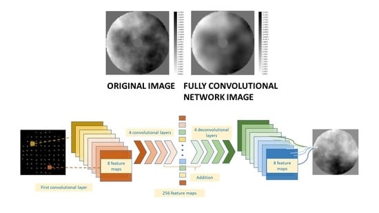
The CNN model chose for the experiment consisted in a convolutional block of 5 convolutional layers where the input images are reduced from 80 pixels by side to 256 features maps of 5 pixels by side. The reduction is made by expanding the strides of the convolutional layers, so pooling layers were not added. Each convolutional layer is formed by 8, 32, 64, 128 and 256 filters respectively, with strides selected to halve the input image size; except for the second layers, which let image shape unchanged. A schematic representation of the CNN model can be found in Figure 3.

Then, after the convolutional block, the 256 filters with 5 × 5 pixels of size are passed to a hidden layer composed by 1200 neurons before being the output layer return the 153 coefficients of the Zernike’s polynomials.

As in the MLP case, all the layers have the selu function as activation function. The ANN was trained for 113 epochs with padding added.

2.4.3. FCN Model

The FCN consist in two main blocks, a convolutional block and a deconvolutional block (see Figure 3). The convolutional block consists in the same as in the previous case, its output of 256 features maps of size 5 × 5 pixels is given to 5 deconvolutional layers. As in the previous block, the size of the outputs is modified by having strides on the deconvolutional layers of size 2 × 2 instead of using transpose pooling layers. All the convolutional transpose layers double the size of the input given except the last one, which receives 8 filters of size 80 × 80 pixels and returns the final output of the ANN, the profile of the turbulence image of size 80 × 80. The rest of deconvolutional layers are formed by 128, 64, 32 and 8 filters.

An additional layer is added between the first and the second deconvolutional layer. The output of the first transpose layer is added with the output of the penultimate convolutional layer, as both outputs have the same number of filters and size, 10 × 10 pixels.

As in the other ANNs, the selu activation function was the chosen one. Padding was added both in the convolutional block as in the other one. The FCN was trained for 115 epochs

3. Results

This section is divided by four subheadings, where the results for the MLP, the CNN and the FCN model are showed separately. The last one consists in an especial test made with the FCN.

3.1. MLP Model

Table 1 shows the results obtained in terms of residual WFE and relative error for the MLP model. The ANN receives the positions of the centroids measured by the SH for each sample, given as output the first 153 coefficients of the Zernike’s polynomials for the turbulence of that moment. Then, the profile of the turbulence phase is reconstructed from the coefficients. It is then compared in terms of the WFE with the one reconstructed from the correct coefficients obtained from the simulation by DASP.

As it has been explained, the network was applied in three test sets where the r₀ value was fixed for each one; for each combination, a total of 3000 samples were taken into consideration:

Table 1. Results obtained for the MLP model. Each value is obtained as the mean value over the 3000 samples of the test dataset.

${\mathit{r}}_0\mathbf{Value}\left(\mathbf{cm}\right)$	Residual RMSE WFE (nm)	Relative Residual RMSE WFE (%)	Original RMSE WFE (nm)	Network RMSE WFE (nm)
$r_0=8$	100.84	28	357.53	289.28
$r_0=10$	90.65	30	297.43	230.20
$r_0=12$	84.54	33	255.67	187.42

Table 1. Results obtained for the MLP model. Each value is obtained as the mean value over the 3000 samples of the test dataset.

${\mathit{r}}_0\mathbf{Value}\left(\mathbf{cm}\right)$	Residual RMSE WFE (nm)	Relative Residual RMSE WFE (%)	Original RMSE WFE (nm)	Network RMSE WFE (nm)
$r_0=8$	100.84	28	357.53	289.28
$r_0=10$	90.65	30	297.43	230.20
$r_0=12$	84.54	33	255.67	187.42

Further, the average of the computational time per sample is showed in the

Table 2. Means of the computational time needed by the MLP model per sample for each test dataset.

Dataset	Computational Time per Sample (ns)
$r_0=8\mathrm{cm}$	230
$r_0=10\mathrm{cm}$	238
$r_0=12\mathrm{cm}$	243

for each of the cases

3.2. CNN Model

The results obtained for the convolutional neural network are showed in

Table 3. Results obtained for the CNN model. Each value is obtained as the mean value over the 3000 samples of the test dataset.

${\mathit{r}}_0\mathbf{Value}\left(\mathbf{cm}\right)$	Residual RMSE WFE (nm)	Relative Residual RMSE WFE (%)	Original RMSE WFE (nm)	Network RMSE WFE (nm)
$r_0=8$	86.58	24	357.53	299.47
$r_0=10$	104.91	35	297.43	208.81
$r_0=12$	112.05	44	255.67	155.84

, with the corresponding computational time needed in

Table 4. Means of the computational time needed by the MLP model per sample for each test dataset.

Dataset	Computational Time per Sample (ns)
$r_0=8\mathrm{cm}$	575
$r_0=10\mathrm{cm}$	600
$r_0=12\mathrm{cm}$	575

. In this case, the input of the network were directly the images received on each subaperture of the SH, giving as output the first 153 coefficients of the Zernike’s polynomials; for each combination, a total of 3000 samples were taken into consideration.

As in the MLP case, from the Zernike’s coefficient the image of the profile of the turbulence phase is reconstructed to calculate de residual WFE made by the ANN.

3.3. FCN Model

In this case the ANN receives as inputs the images received by the subapertures of the SH given directly as output the image of the profile of the turbulence phase. Therefore, the residual WFE showed in the results corresponds straightaway with the comparison between the real profile of the turbulence phase simulated by DASP and the one predicted by the FCN. The results are shown in

Table 5. Results obtained for the FCN model. Each value is obtained as the mean value over the 3000 samples of the test dataset. In this case, the output of the ANN is directly compared with the simulated image of the phase’s profile by DASP.

${\mathit{r}}_0\mathbf{Value}\left(\mathbf{cm}\right)$	Residual RMSE WFE (nm)	Relative Residual RMSE WFE (%)	Original RMSE WFE (nm)	Network RMSE WFE (nm)
$r_0=8$	253.63	19	1310.93	1251.85
$r_0=10$	191.50	18	1088.87	1058.32
$r_0=12$	160.94	17	935.07	915.71

; for each combination, a total of 3000 samples were taken into consideration.

In

Table 6. Means of the computational time needed by the FCN model per sample for each test dataset.

Dataset	Computational Time per Sample (ns)
$r_0=8\mathrm{cm}$	675
$r_0=10\mathrm{cm}$	700
$r_0=12\mathrm{cm}$	678

the computational time needed per sample by the FCN is showed.

3.4. FCN Model for Profile Phase Approximation

An extra text was made to compare the performance of the FCN due to the difference in the output given by each kind of ANN. In the case of the FCN model, its outputs contain much more information (an image of 80 × 80 pixels) than the others, as they only calculate 153 values corresponding with the 153 first Zernike’s coefficients; for each combination, a total of 3000 samples were taken into consideration. In this subsection, the same FCN topology as in Section 3.3 was tested but, the output given corresponds with the profile of the phase calculated from the first 153 Zernike’s modes simulated by DASP. Therefore, for that test, the same information is given by the FCN in comparison with the others ANN models.

The phase was reconstructed from the same test datasets as in previous chapters and then it is compared with the output of the FCN in terms of WFE and similarity. The results are shown in

Table 7. Results obtained for the FCN model, when reconstructing the approximated profile of the phase. Each value is obtained as the mean value over the 3000 samples of the test dataset.

${\mathit{r}}_0\mathbf{Value}\left(\mathbf{cm}\right)$	Residual RMSE WFE (nm)	Relative Residual RMSE WFE (%)	Original RMSE WFE (nm)	Network RMSE WFE (nm)
$r_0=8$	146.68	37	394.19	302.52
$r_0=10$	177.23	44	395.21	256.69
$r_0=12$	203.72	52	394.08	224.09

while the computational times needed are shown in

Table 8. Means of the computational time needed by the FCN model per sample for each test dataset.

Dataset	Computational Time per Sample (ns)
$r_0=8\mathrm{cm}$	675
$r_0=10\mathrm{cm}$	670
$r_0=12\mathrm{cm}$	675

.

4. Discussion

The results of different kinds of ANN models have been compared for the same problem in order to determine which one could be the most profitable model for night SCAO reconstructions.

In terms of the computational time needed to make the reconstructions, the results showed how the MLP is the quickliest model, being approximately 40% quicker than the CNN model and the double than FCN ones. That result could be expected as the problem resolved by the MLP is the simplest one, passing from an input of 160 values (the positions of the not darkened subapertures centroids) to an output of 153 values. Therefore, it does not have to interpret an image with the corresponding waste of time. The CNN corresponds with the intermediate case when talking of computational time needed since, although it interprets the whole image of the subapertures, it does not generate a new image as output, a fact that the FCN does.

The other term to analyze is the quality of the reconstructions made by each of the models. For this analysis a separation between the different cases is needed since it is not the same problem reconstructing an approximation of the turbulence phase with the 153 first Zernike’s mode than all the information contained in the turbulence phase. Therefore, the results showed in the Section 3.1, Section 3.2 and Section 3.4 are firstly compared.

When the objective is to obtain an approximation of the information contained in the profile of the turbulence phase, the CNN showed the best results of the three compared. For the most turbulence case tested with an $r_0$ value of 8 cm, the CNN commits a mean relative WFE of 24% being a 44% in the cases o lowest turbulence. An example randomly chosen over the 4000 samples of the test set is showed in Figure 4 and Figure 5. The result is closely followed by the MLP model, that is able to achieve a mean relative WFE of 28% in the highest turbulence case and a 33% in the lowest one. Therefore, in cases of soft turbulences, the MLP achieves the lowest errors. The worst model in this kind of reconstruction is clearly the FCN one, as it achieves a 37% of relative error in the most turbulence case being increased to a 52% in the most turbulence. An example of that is showed in Figure 6.

It is important to remark that all the error committed is due to the reconstruction made by the ANNs and not to the approximation. The images that are compared to are obtained from the 153 Zernike’s modes simulated by DASP. They do not correspond directly with the original turbulence phase simulated.

For these tests, both the CNN and the FCN have much information on their inputs in comparison with the MLP, to obtain an output that corresponds with an approximation made with not a lot of information. That fact could make that the convolutional block (that it’s the same for both of them) is not able to extract the main characteristics to make relationship with the phase. That is observed especially in the FCN case, where the ANN has to extract characteristics from a lot information to obtain an extended output (an image of 80 × 80 pixels) that contains a little of information. In that point resides the amount of error obtained by the FCN.

These three cases differ with the result showed in the Section 3.3 (example in Figure 7), where the FCN recovers the image of the phase profile that contains all the information possible. In this situation, the same FCN model achieves only a 19% of relative WFE for the $r_0=8 \mathrm{cm}$ test and a 17% in the $r_0=12 \mathrm{cm}$ case. Therefore, the FCN is able to relation the information received with the output when the last one contains enough information.

Furthermore, a change on the trend with the $r_0$ value is observed between the first three cases analyzed and the last one. When the output contains less information, the error committed by the ANN increases when the turbulence intensity decreases, since for lights turbulences making relations among the information received and the main characteristics of the turbulence is more difficult. That is not the situation of the FCN, as the output contains enough information in all the cases to make the relations and the trend shows that the error decreases with the turbulence intensity, probably due to the fact that the phase of the turbulence phase needs less precision being the aberrations longer and more continuous.

5. Conclusions

In this paper, a comparison between the most used kinds of ANNs has been made, for one of the nocturnal AO configurations, the SCAO configuration. The research consists of a proof of concept in order to obtain a strategy for which type of neural network could fit the best in AO problems, to determine which one could be the most profitable to develop for future AO systems in next generation telescopes that are already under construction, for example, for the case of solar AO.

In AO, the most important parameters of a RS are such the computational time needed as the errors made in the reconstruction. The comparison is made in both terms, giving different results according to each factor.

In terms of computational time, the MLP model achieves up to three times faster computational times than the CNN, being even higher in the FCN case. The MLP do not have to process images, only arrays of numbers, so that is an expected result. However, in the comparison the time needed by the SH to calculate centroids of each subaperture is not being considered. The operation consists in correlation between the light received by the CCD pixels, not involving a high computational cost. Due to the simplicity of the operations that are made by MLPs compared to the other models, their reconstructions should continue to be the fastest ones.

On the other hand, the WFE errors of the reconstructions show another trend between the different models. When an approximation of the phase by 153 Zernike’s modes is reconstructed, the CNN shows results that fit the most with the original phases when high turbulence intensities are present. The MLP model achieves similar results but the WFE is a bit higher. However, the less intensity of turbulence there is, the lower the WFE obtained by the MLP compared with the CNN one. Therefore, the CNN takes advantage of having all the image received by the SH as input when it is very aberrated by the turbulence, as more information of the last one is contained in the image. If the aberrations are lower, CNN will not be able to get lower WFE than the MLP.

This trend could be modified in future developments in Solar AO, as the images receives by the SH consists in a region of the sun, instead of a blurred point from the source of the light. Those images contain much more information even in low turbulence cases (as all the region of the sun is aberrated instead of a point). According to the test made along this research, the use of CNN when the SH’s subapertures receives images with a wide amount of information achieves better results than the MLP.

Finally, the results obtained by the FCN are presented, where they show high values of WFE when the objective is to reconstruct an approximation of the turbulence phase based on 153 Zernike’s modes, as in the previous cases. The FCN achieves 37% of relative error in high intensity turbulences, increasing the relative error in low intensities ones. In addition, another scenario was considered. This new experiment contains much more information of the turbulence than the approximations of the previous comparisons and, for this case, the FCN shows the best results of all the test made, achieving only a 19% of relative WFE for high turbulences. This error decreases until 15% in lower turbulence cases, much better than any other model.

From the last result it is possible to conclude that the FCN is the model that best fits to the AO system, as it reconstructs much more information than any other model and giving the lower relative error. Nevertheless, the objective of an RS system is to give the necessary turbulence information to a DM to correct the aberrations. The information is passed to a DM as an array of values, typically the needed voltages of the actuators. Anyway, whatever the format of the values, the result objective of an RS approximates the turbulence with some values, so the output of the FCN, despite having more information than any other ANN model, will have to be reduced for being useful. This process will increase the computational time needed by the RS but the error will be reduced, as in approximations the output of the FCN will be more similar to the original phase than in a completely reconstructed image with all the details.

Possible improvements and future work from this research are the improvement of ANNs models to decrease the actual error, as well as performing this study in other scenarios such as solar AO systems, to check if the expected performance of both ANNs with convolutional blocks would be improved working with extended images in the SH, with the corresponding challenges of the implementation of ANN models in these systems.