Rigorous Mathematical Investigation of a Nonlocal and Nonlinear Second-Order Anisotropic Reaction-Diffusion Model: Applications on Image Segmentation

Abstract

In this paper we are addressing two main topics, as follows. First, a rigorous qualitative study is elaborated for a second-order parabolic problem, equipped with nonlinear anisotropic diffusion and cubic nonlinear reaction, as well as non-homogeneous Cauchy-Neumann boundary conditions. Under certain assumptions on the input data: $f(t,x)$, $w(t,x)$ and $v_0\left(x\right)$, we prove the well-posedness (the existence, a priori estimates, regularity, uniqueness) of a solution in the Sobolev space $W_p^{1,2}\left(Q\right)$, facilitating for the present model to be a more complete description of certain classes of physical phenomena. The second topic refers to the construction of two numerical schemes in order to approximate the solution of a particular mathematical model (local and nonlocal case). To illustrate the effectiveness of the new mathematical model, we present some numerical experiments by applying the model to image segmentation tasks.

1. Introduction

For the unknown function $v(t,x)$ (hereafter, v), consider the following nonlinear second-order boundary value problem in $Q=(0,T]\times \mathsf{\Omega }$, with $T>0$ and a bounded domain $\mathsf{\Omega }\subset I{R}^2$ of Lebesgue measures $\left|\mathsf{\Omega }\right|$, whose boundary $\partial \mathsf{\Omega }$ is sufficiently smooth:

$$\left\{\begin{array}{c}{\displaystyle p_{{}_1}\frac{\partial }{\partial t}v(t,x)=\mathsf{\Phi }\left(v_x(t,x)\right)\left[\mathsf{\Psi }\left(v_x(t,x)\right)\mathsf{\Delta }v(t,x)+\mathsf{\nabla }\mathsf{\Psi }\left(v_x(t,x)\right)·\mathsf{\nabla }v(t,x)\right]}\hfill \\ \\ +p_{{}_3}\left[v(t,x)-v^3(t,x)\right]+p_{{}_4}f(t,x)\hfill & \mathrm{in}Q\hfill \\ \\ {\displaystyle \overline{q}(t,x)\frac{\partial }{\partial \mathbf{n}}v(t,x)+p_{{}_5}v(t,x)=w(t,x)}\hfill & \mathrm{on}\mathsf{\Sigma }\hfill \\ \\ v(0,x)=v_0\left(x\right)\hfill & \mathrm{on}\mathsf{\Omega },\hfill \end{array}\right.$$

(1)

where:

• $t\in (0,T]$, $x=(x_1,x_2)$ varies in $\mathsf{\Omega }$, $\mathsf{\Sigma }=(0,T]\times \partial \mathsf{\Omega }$;
• $\mathsf{\nabla }v(t,x)=v_{{}_x}(t,x)$ ($\mathsf{\nabla }v=v_{{}_x}$) the gradient of $v(t,x)$ in x, that is ${\displaystyle \mathsf{\nabla }v=\left(\frac{\partial }{\partial x_1}v,\frac{\partial }{\partial x_2}v\right)}$. Setting ${\displaystyle \frac{\partial }{\partial x_i}v=v_{x_i}}$, $i=1,2$, then $\mathsf{\nabla }v=\left(v_{{}_{x_1}},v_{{}_{x_2}}\right)=v_{{}_x}$;
• $\mathsf{\Delta }v(t,x)$ is the Laplace operator—a second-order differential operator, defined as the divergence ($\mathsf{\nabla }·$) of the gradient of $v(t,x)$ in x;
• ${\displaystyle \frac{\partial }{\partial t}v(t,x)}$ is the partial derivative of $v(t,x)$ with respect to t;
• $p_{{}_1},p_{{}_3},p_{{}_4},p_{{}_5}$ are positive values.
• $\mathsf{\Phi }\left(v_x(t,x)\right)$ is a positive and bounded nonlinear real function of class $C^1\left(Q\right)$ with bounded derivatives (see [1]), having the role of controlling the speed of the diffusion process and enhances the edges (e.g., in the evolving image);
• $\mathsf{\Psi }\left(v_x(t,x)\right)$ is the mobility;
• $\overline{q}(t,x)$ is a positive and bounded real function;
• $f(t,x)\in L^p\left(Q\right)$ is the distributed control (a given function), where

  $$p\ge 2;$$

  (2)
• $w(t,x)\in W_p^{1-\frac{1}{2p},2-\frac{1}{p}}\left(\mathsf{\Sigma }\right)$ is the boundary control (a given function);
• n = n(x) is the outward unit normal vector to $\mathsf{\Omega }$ at a point $x\in \partial \mathsf{\Omega }$. $\frac{\partial }{\partial \mathbf{n}}$ denotes differentiation along n;
• $v_0\left(x\right)\in W_p^{2-\frac{2}{p}}\left(\mathsf{\Omega }\right)$, verifying

  $${\displaystyle \overline{q}(t,x)\frac{\partial }{\partial \mathbf{n}}{v}_0\left(x\right)+p_{{}_5}{v}_0\left(x\right)=w(0,x).}$$

  (3)

Let us note

$$a_i(t,x,v(t,x),v_x(t,x))=\mathsf{\Phi }\left(v_x(t,x)\right)\mathsf{\Psi }\left(v_x(t,x)\right)v_{{}_{x_i}}(t,x),i=1,2.$$

(4)

Then, it is easy to recognize Equation (1)${}_1$ as being quasi-linear with

$${\displaystyle \begin{array}{cc}{\displaystyle a_{ij}\left(t,x,v(t,x),v_x(t,x)\right)}\hfill & {\displaystyle =\frac{\partial }{\partial v_{{}_{x_j}}}{a}_i\left(t,x,v(t,x),v_x(t,x)\right)}\hfill \\ \hfill & {\displaystyle =\frac{\partial }{\partial v_{{}_{x_j}}}\mathsf{\Phi }\left(v_x(t,x)\right)\mathsf{\Psi }\left(v_x(t,x)\right)v_{x_i}(t,x),i=1,2,}\hfill \\ {\displaystyle a\left(t,x,v(t,x),v_x(t,x)\right)}\hfill & {\displaystyle =-\frac{\partial }{\partial v}\left(\mathsf{\Phi }\left(v_x(t,x)\right)\mathsf{\Psi }\left(v_x(t,x)\right)v_{x_i}(t,x)\right)v_{x_i}(t,x)}\hfill \\ & {\displaystyle -\frac{\partial }{\partial x_i}\mathsf{\Phi }\left(v_x(t,x)\right)\mathsf{\Psi }\left(v_x(t,x)\right)v_{x_i}(t,x)}\hfill \\ & {\displaystyle -p_{{}_3}\left[v(t,x)-v^3(t,x)\right]-p_{{}_4}f(t,x),}\hfill \end{array}}$$

while the boundary conditions (1)${}_2$ are of second type:

$${\left[a_{ij}\left(t,x,v(t,x),v_x(t,x)\right)v_{x_j}(t,x)cos{\alpha }_i+p_{{}_5}v(t,x)-w(t,x)\right]}_{{}_{\mathsf{\Sigma }}}=0,$$

(see [1] and reference therein).

For the reader’s benefit, we write problem (1) in the equivalent form

$$\left\{\begin{array}{c}{\displaystyle p_{{}_1}\frac{\partial }{\partial t}v(t,x)-\mathsf{\Phi }\left(v_x(t,x)\right)\mathrm{div}\left(\mathsf{\Psi }\left(v_x(t,x)\right)\mathsf{\nabla }v(t,x)\right)}\hfill \\ \\ =p_{{}_3}\left[v(t,x)-v^3(t,x)\right]+p_{{}_4}f(t,x)\hfill & \mathrm{in}Q\hfill \\ \\ {\displaystyle \overline{q}(t,x)\frac{\partial }{\partial \mathbf{n}}v(t,x)+p_{{}_5}v(t,x)=w(t,x)}\hfill & \mathrm{on}\mathsf{\Sigma }\hfill \\ \\ v(0,x)=v_0\left(x\right)\hfill & \mathrm{on}\mathsf{\Omega }.\hfill \end{array}\right.$$

(5)

Concerning Equation (5)${}_1$, we recall that it is of quasi-linear type with principal part in divergence form (see [1]), with $a_i$, $i=1,2$, given by (4) and

$a(t,x,v(t,x),v_x(t,x))=-p_{{}_3}\left[v(t,x)-v^3(t,x)\right]-p_{{}_4}f(t,x)$.

In addition, we assume that Equations (1)${}_1$ [or (5)${}_1$] are uniformly parabolic, i.e.,

$${\nu }_{{}_1}\left(\right|u\left|\right){\zeta }^2\le a_{ij}\left(t,x,u,z\right){\zeta }_i{\zeta }_j\le {\nu }_{{}_2}\left(\right|u\left|\right){\zeta }^2$$

(6)

for arbitrary $u(t,x)$ and $z(t,x)$, $(t,x)\in Q$, and $\zeta =({\zeta }_1,{\zeta }_2)$ an arbitrary real vector, where ${\nu }_{{}_1}\left(s\right)$, ${\nu }_{{}_2}\left(s\right)$ are positive continuous functions of $s\ge 0$, ${\nu }_{{}_1}\left(s\right)$ is nonincreasing and ${\nu }_{{}_2}\left(s\right)$ is nondecreasing.

The nonlinear problem (1) (or (5)) is important for modeling a variety of phenomena of life sciences, including in biology, biochemistry, economics, medicine and physics. Particular cases of the nonlinear second-order boundary value problem (1), supplied with different boundary conditions, have been successfully applied to many complex moving interface problems, e.g., the motion of anti-phase boundaries in crystalline solids [2], the mixture of two incompressible fluids, the nucleation of solids, and vesicle membranes (see [3,4,5] and the references therein). In addition, the nonlinear problems of type (1)${}_1$, occur in the phase-field transition system (e.g., [6]) where the phase function $v(t,x)$ describes the transition between the solid and liquid phases in the solidification process of a material occupying a region $\mathsf{\Omega }$. For more general assumptions and with various types of boundary conditions, Equation (5) has been numerically investigated (e.g., [6,7,8,9,10,11,12,13,14,15,16,17]). The error analysis for the implicit backward Euler approximation is presented in [16], and computations with several different higher-order time-stepping schemes are used in [11]. For the well-posedness (existence, estimate, uniqueness and regularity) of a solution in Sobolev spaces we refer to [12,18,19,20,21].

Another important novelty in our paper concerns the non-homogeneous Cauchy-Neumann boundary conditions, which can be seen as boundary control in industry. Thus, as applications of problem (1), we indicate the moving interface problems, e.g., phase separation and transition (see [3,8,12,17,18,22,23,24,25,26,27]), anisotropy effects (see [15,28,29,30]), image denoising and segmentation (see [15,24,26,30,31,32,33,34,35,36,37,38,39] and references therein), etc.

Definition 1.

The function $v(t,x)$ is called a classical solution of the problem (1) if it is continuous in $\overline{Q}$, has continuous derivatives $v_t$, $v_x$, $v_{xx}$ in Q, verifies (1)${}_1$ in every $(t,x)\in Q$ and verifies (1)${}_2$ and (1)${}_3$ for $(t,x)\in \mathsf{\Sigma }$ and $t=0$, respectively.

In our paper, we study the solvability of the problems (1) in the class $W_p^{1,2}\left(Q\right)$, characterized by the presence of some new physical parameters ($p_{{}_1}$, $p_{{}_3}$, $p_{{}_4}$, $p_{{}_5}$, $\mathsf{\Phi }\left(v_x(t,x)\right)$, $\mathsf{\Psi }\left(v_x(t,x)\right)$), the principal part being in divergence form and by considering the cubic nonlinearity $p_{{}_3}\left[v(t,x)-v^3(t,x)\right]$, satisfying for $n\in \{1,2,3\}$ the assumption $H_0$ in [21], that is: $H_0:$$(v-v^3){\left|v\right|}^{3p-4}v\le 1+{\left|v\right|}^{3p-1}-{\left|v\right|}^{3p}.$

In Theorem 1, we prove the existence, regularity and uniqueness of solution for (1). (see [15] for a numerical study of Equation (1) corresponding to a linear reaction term $v(t,x)-v_0\left(x\right)$, with homogeneous Neumann boundary condition).

In the following we will denote by C several positive constants.

2. Well-Posedness of the Solution of (5)

Theorem 1 of this section presents the dependence of the solution $v(t,x)$ of (5) on $f(t,x)$ and $w(t,x)$. In our study, we rely on the following:

• The Leray-Schauder principle (see [1,4,11,12,13,14,15,19,20,21] and reference therein);
• The $L^p$-theory of linear and quasi-linear parabolic equations;
• Green’s first identity
  ${\displaystyle -\underset{\mathsf{\Omega }}{\int }y\mathrm{div}zdx=\underset{\mathsf{\Omega }}{\int }\mathsf{\nabla }y·zdx-\underset{\partial \mathsf{\Omega }}{\int }y\frac{\partial }{\partial \mathbf{n}}zd\gamma }$,
  ${\displaystyle -\underset{\mathsf{\Omega }}{\int }y\mathsf{\Delta }zdx=\underset{\mathsf{\Omega }}{\int }\mathsf{\nabla }y·\mathsf{\nabla }zdx-\underset{\partial \mathsf{\Omega }}{\int }y\frac{\partial }{\partial \mathbf{n}}zd\gamma }$,
  for any scalar-valued function y and z, a continuously differentiable vector field in n dimensional space;
• The Lions and Peetre embedding theorem (see [1] and references therein) to ensure the existence of a continuous embedding $W_p^{1,2}\left(Q\right)\subset L^{\mu }\left(Q\right)$, where the number $\mu$ is defined as follows (see (3))

  $$\mu =\left\{\begin{array}{cc}\mathrm{any}\mathrm{positive}\mathrm{number}\ge 3p\hfill & \mathrm{if}p\ge 2,\hfill \\ \\ {\displaystyle {\left(\frac{1}{p}-\frac{1}{2}\right)}^{-1},}\hfill & \mathrm{if}p<2.\hfill \end{array}\right.$$

  (7)

  and, for $k\in \{1,2,\dots \}$ and $1\le p\le \infty$, $W_p^{k,2k}\left(Q\right)$ denotes the Sobolev space on Q:

  $$W_p^{k,2k}\left(Q\right)=\left\{y\in L^p\left(Q\right):{\displaystyle }\frac{{\partial }^r}{\partial t^r}{\displaystyle }\frac{{\partial }^q}{\partial x^q}y\in L^p\left(Q\right),\mathrm{for}2r+q\le 2k\right\},$$

  (8)
  (see [1] for more details).

In addition, we use the set $C^{1,2}\left(\overline{Q}\right)$ ($C^{1,2}\left(Q\right)$) of all continuous functions in $\overline{Q}$ (in Q) having continuous derivatives $u_t$, $u_x$ and $u_{xx}$ in $\overline{Q}$ (in Q), as well as the Sobolev spaces $W_p^l\left(\mathsf{\Omega }\right)$, $W_p^{l,l/2}\left(\mathsf{\Sigma }\right)$ with non-integral l for the initial and boundary conditions, respectively (see [1]).

The main result for the study of the existence, a priori estimates, uniqueness and regularity for the solution of (1) (or (5)) is the next theorem.

Theorem 1.

For any classical solution $v(t,x)\in C^{1,2}\left(Q\right)$ of (5), suppose there are M, $M_{{}_0}$, $m_{{}_1}$, $M_{{}_1}$, $M_{{}_2}$, $M_{{}_3}$ and $M_{{}_4}\in (0,\infty )$ such that the fpllowing hypotheses are satisfied:

I${}_1$. $\left|v\right(t,x\left)\right|<M$ for any $(t,x)\in Q$ and for any $z(t,x)$, the map $\mathsf{\Psi }\left(z\right(t,x\left)\right)$ is continuous, differentiable in x, its x-derivatives are measurable bounded, satisfies (6) and

$$0<{\mathsf{\Psi }}_{min}\le \mathsf{\Psi }\left(v_x(t,x)\right)<{\mathsf{\Psi }}_{max},for(t,x)\in Q,$$

(9)

$$\begin{array}{cc}\hfill & {\displaystyle |\mathsf{\Psi }\left(z\right)v_{x_i}\left|\right(1+\left|z\right|)+\left|{\displaystyle \frac{\partial }{\partial x_1}}\left(\mathsf{\Psi }\left(z\right)v_{x_1}\right)\right|+\left|\frac{\partial }{\partial x_2}\left(\mathsf{\Psi }\left(z\right)v_{x_1}\right)\right|}\hfill \\ \\ \hfill & +\left|{\displaystyle \frac{\partial }{\partial x_1}}\left(\mathsf{\Psi }\left(z\right)v_{x_2}\right)\right|+\left|{\displaystyle \frac{\partial }{\partial x_2}}\left(\mathsf{\Psi }\left(z\right)v_{x_2}\right)\right|+|v(t,x_1,x_2)|\le M_{{}_0}{(1+|z\left|\right)}^2.\hfill \end{array}$$

(10)

I${}_2$. $\mathsf{\Phi }\left(v_x(t,x)\right)$ is a positive and bounded nonlinear real function of class $C^1\left(Q\right)$ with bounded derivatives and

   0 < $m_{{}_1}\le \mathsf{\Phi }\left(v_x(t,x)\right)\le M_{{}_1}$.

In addition, for every $\epsilon >0$, the functions $v(t,x)$ and $\mathsf{\Psi }\left(v_x(t,x)\right)$ satisfy the relations

   ${\parallel v\parallel }_{{}_{L^s\left(Q\right)}}\le M_{{}_2}$, $\parallel \mathsf{\Psi }\left(v_x\right)v_{x_i}{\parallel }_{{}_{L^r\left(Q\right)}}<M_{{}_3},i=1,2,$

where

$$\begin{array}{cc}r=\left\{\begin{array}{cc}max\{p,4\}\hfill & p\ne 4\hfill \\ 4+\epsilon \hfill & p=4,\hfill \end{array}\right.\hfill & s=\left\{\begin{array}{cc}max\{p,2\}\hfill & p\ne 2\hfill \\ 2+\epsilon \hfill & p=2.\hfill \end{array}\right.\hfill \end{array}$$

Then, $\forall f\in L^p\left(Q\right)$ and $\forall v_0\in W_p^{2-\frac{2}{p}}\left(\mathsf{\Omega }\right)$, with $p\ne \frac{3}{2}$, the problem (5) has a solution $v\in W_p^{1,2}\left(Q\right)$ and the next estimate holds:

$$\begin{array}{cc}\hfill & {\parallel v\parallel }_{W_p^{1,2}\left(Q\right)}\le C\left[1+\parallel v_0{\parallel }_{W_p^{2-\frac{2}{p}}\left(\mathsf{\Omega }\right)}+{\parallel v_0\parallel }_{L^{3p-2}\left(\mathsf{\Omega }\right)}^{3-\frac{2}{p}}\right.\hfill \\ \\ \hfill & \left.+{\parallel f\parallel }_{L^p\left(Q\right)}+{\parallel w\parallel }_{L^{3p-2}\left(\mathsf{\Sigma }\right)}^{3-\frac{2}{p}}+{\parallel w\parallel }_{W_p^{1-\frac{1}{2p},2-\frac{1}{p}}\left(\mathsf{\Sigma }\right)}\right],\hfill \end{array}$$

(11)

where the constant $C>0$ does not depend on $v,f$ and w.

If $v^1,v^2\in W_p^{1,2}\left(Q\right)$ are two solutions to (5), corresponding to $\{f^1,w^1,v_0^1\}$ and $\{f^2,w^2,v_0^2\}$, respectively, such that $\parallel v^1{\parallel }_{W_p^{1,2}\left(Q\right)}\le M_{{}_4}$, $\parallel v^2{\parallel }_{W_p^{1,2}\left(Q\right)}\le M_{{}_4}$ and

$$0<q_{min}\le \overline{q}(t,x)<q_{max},for(t,x)\in \mathsf{\Sigma },$$

(12)

then the following estimate holds:

$$\begin{array}{c}{\displaystyle \underset{(t,x)\in Q}{max}|v^1-v^2|\le C_1{e}^{CT}max\left[{\displaystyle \underset{(t,x)\in Q}{max}|f^1-f^2|,\underset{(t,x)\in \mathsf{\Sigma }}{max}|w^1-w^2|,\underset{(t,x)\in \mathsf{\Omega }}{max}|v_0^1-v_0^2|}\right],}\hfill \end{array}$$

(13)

where the constant C, $C_1>0$ does not depend on $\{v^1,f^1,w^1,v_0^1\}$ and $\{v^2,f^2,w^2,v_0^2\}$. In particular, the solution of problem (5) is unique.

2.1. The Proof of Theorem 1

To prove this theorem, we use the Leray-Schauder principle. Thus, we consider the Banach space

$$B=W_p^{0,1}\left(Q\right)\cap L^{3p}\left(Q\right),$$

endowed with the norm

$${\parallel u\parallel }_B={\parallel u\parallel }_{L^p\left(Q\right)}+{\parallel u_x\parallel }_{L^p\left(Q\right)},$$

and a nonlinear operator $H:B\times [0,1]\to B$ defined by

$$v=v(u,\lambda )=H(u,\lambda )\mathrm{for}\mathrm{all}(u,\lambda )\in W_p^{0,1}\left(Q\right)\cap L^{3p}\left(Q\right)\times [0,1],$$

(14)

where $v(u,\lambda )$ is the unique solution to the next problem

$$\left\{\begin{array}{c}{p}_{{}_1}{\displaystyle \frac{\partial }{\partial t}}v(t,x)-\left[\lambda \mathsf{\Phi }\left(u_x(t,x)\right){\displaystyle \frac{\partial }{\partial u_{x_j}}}\left(\mathsf{\Psi }\left(u_x\right)u_{x_i}\right)+(1-\lambda ){\delta }_i^j\right]v_{x_i{x}_j}\hfill \\ \\ =\lambda \left\{A(t,x,u,u_x)+p_{{}_3}\left[u(t,x)-u^3(t,x)\right]+p_{{}_4}f(t,x)\right\}\hfill & \mathrm{in}Q\hfill \\ \\ \overline{q}(t,x){\displaystyle \frac{\partial }{\partial \nu }}v(t,x)+p_{{}_5}v(t,x)=\lambda w(t,x)\hfill & \mathrm{on}\mathsf{\Sigma }\hfill \\ \\ v(0,x)=\lambda v_0\left(x\right),\hfill & \mathrm{on}\mathsf{\Omega }.\hfill \end{array}\right.$$

(15)

with $A(t,x,u,u_x)=\mathsf{\Phi }\left(u_x\right)\mathsf{\nabla }\mathsf{\Psi }\left(u_x\right)·\mathsf{\nabla }u$, $\forall (t,x)\in Q$.

We shall prove now the following technical lemma

Lemma 1.

We assume Hypotheses I${}_1$ and I${}_2$ to be valid. Then

$$A(t,x,u,u_{x_i})+p_{{}_3}(u-u^3)+p_{{}_4}f(t,x)\in L^p\left(Q\right),\forall u\in W_p^{0,1}\left(Q\right)\cap L^{3p}\left(Q\right).$$

(16)

Proof. 

Indeed, since $u\in L^{3p}\left(Q\right)$, then ${\parallel u\parallel }_{L^{3p}\left(Q\right)}\le Konst$ and thus

$$\parallel u^3{\parallel }_{L^p\left(Q\right)}={\left(\underset{Q}{\int }{\left|u^3\right|}^{p}dxdt\right)}^{\frac{1}{p}}={\left[{\left(\underset{Q}{\int }{\left|u\right|}^{3p}dxdt\right)}^{\frac{1}{3p}}\right]}^{3p\frac{1}{p}}={\parallel u\parallel }_{L^{3p}\left(Q\right)}^3\le {\left(Konst\right)}^3,$$

i.e., the nonlinear term in (16) belongs to $L^p\left(Q\right)$, $\forall u\in W_p^{0,1}\left(Q\right)\cap L^{3p}\left(Q\right)$ (see also [1]).

Next, from (10) it is easy to conclude that

$\frac{\partial }{\partial x_i}\left[\mathsf{\Psi }\left(u_{x_i}\right)u_{x_i}\right]\le M_{{}_1}(1+|u_{x_i}{\left|\right)}^2$.

Thus, to prove that

$A(t,x,u,u_{x_i}))=\mathsf{\Phi }\left(u_x(t,x)\right)\mathsf{\nabla }\mathsf{\Psi }\left(u_x(t,x)\right)·\mathsf{\nabla }u(t,x)\in L^p\left(Q\right)$,

$\forall u\in W_p^{0,1}\left(Q\right)\cap L^{3p}\left(Q\right),$

we have to prove that $u_{x_i}^2\in L^p\left(Q\right)$, $\forall u\in W_p^{0,1}\left(Q\right)\cap L^{3p}\left(Q\right)$. For any $u\in W_p^{0,1}\left(Q\right)\cap L^{3p}\left(Q\right)$ it follows that ${\parallel u\parallel }_{L^p\left(Q\right)}+{\parallel u_x\parallel }_{L^p\left(Q\right)}\le konst$, i.e., $\parallel u_x{\parallel }_{L^p\left(Q\right)}\le konst$. Making use of the boundedness of $\mathsf{\Phi }\left(u_x(t,x)\right)$ (see I${}_2$), as well as the properties of $\mathsf{\Psi }\left(u_x(t,x)\right)$ (see I${}_1$), and since $u_{x_i}\in L^p\left(Q\right)$, it results that $A(t,x,u,u_{x_i})\in L^p\left(Q\right)$, $\forall u\in W_p^{0,1}\left(Q\right)\cap L^{3p}\left(Q\right)$.

Finally, we recall that $f(t,x)\in L^p\left(Q\right)$ and, owing to the above, we easy derive that the statement expressed by (16) is true. □

2.2. The Proof of Theorem 1 (Continued)

Let us show that the nonlinear operator $H(u,\lambda )$ defined by (14) satisfies the following Properties A and B.

A. 

If (15) has a unique solution, then H is well-defined. By the right hand of ${\left(15\right)}_1$, using Lemma 1, it follows that, $\forall u\in W_p^{0,1}\left(Q\right)\cap L^{3p}\left(Q\right)$, then $A(t,x,u,u_x)+p_{{}_3}(u-u^3)+p_{{}_4}f(t,x)\in L^p\left(Q\right)$ and thus, the same reasoning as in [1] allows us to conclude that for $w(t,x)\in W_p^{2-\frac{1}{p},1-\frac{1}{2p}}\left(\mathsf{\Sigma }\right)$, the linear parabolic boundary value problem formulated in (15) has a unique solution, that is (see (14)) $v=H(u,\lambda )\in W_p^{1,2}\left(Q\right)$, $\forall u\in B$ and $\forall \lambda \in [0,1]$. Next, the embedding $W_p^{1,2}\left(Q\right)\subset L^{\mu }\left(Q\right)\subset L^{3p}\left(Q\right)$, $p\ge 2$ (see (3) and (7)), allows us to conclude that

$H(u,\lambda )=v\in B$, $\forall u\in B$ and $\forall \lambda \in [0,1]$.

Thus, the operator H is well-defined.

B. 

Let us now show that H is continuous and compact. The sketch of the proof is the same as in [1,15]. However, for reader convenience, we present details in the sequel. Let $u^n\to u$ in $W_p^{0,1}\left(Q\right)\cap L^{3p}\left(Q\right)$ and ${\lambda }_n\to \lambda$ in $[0,1]$. Making the notation

$$v^{n,{\lambda }_n}=H(u^n,{\lambda }_n),v^{n,\lambda }=H(u^n,\lambda )\mathrm{and}{v}^{\lambda }=H(u,\lambda )$$

and then considering the difference $H(u^n,{\lambda }_n)-H(u^n,\lambda )$, we obtain from relations (14) and (15) that

$$\left\{\begin{array}{cc}{\displaystyle p_{{}_1}\frac{\partial }{\partial t}{V}^{n,{\lambda }_n,\lambda }-\left[\lambda \mathsf{\Phi }\left(u_x^n\right)\frac{\partial }{\partial u_{x_j}^n}\left(\mathsf{\Psi }\left(u_x^n\right)u_{x_i}^n\right)+(1-\lambda ){\delta }_i^j\right]V_{{}_{x_i{x}_j}}^{n,{\lambda }_n,\lambda }}\hfill & \\ \\ =({\lambda }_n-\lambda )\left\{\left[\mathsf{\Phi }\left(u_x^n\right)\frac{\partial }{\partial u_{x_j}^n}\left(\mathsf{\Psi }\left(u_x^n\right)u_{x_i}^n\right)-{\delta }_i^j\right]v_{x_i{x}_j}^{n,{\lambda }_n}\right.\hfill & \\ \\ \left.+A(t,x,u^n,u_{x_i}^n)+p_{{}_3}\left[u^n-{\left(u^n\right)}^3\right]+p_{{}_4}f(t,x)\right\}\hfill & \mathrm{in}Q\hfill \\ \\ \overline{q}(t,x)\frac{\partial }{\partial \mathbf{n}}{V}^{n,{\lambda }_n,\lambda }+p_{{}_5}{V}^{n,{\lambda }_n,\lambda }=({\lambda }_n-\lambda )w(t,x)\hfill & \mathrm{on}\mathsf{\Sigma }\hfill \\ \\ v(0,x)=({\lambda }_n-\lambda )v_0\left(x\right)\hfill & \mathrm{on}\mathsf{\Omega },\hfill \end{array}\right.$$

(17)

where $V^{n,{\lambda }_n,\lambda }=v^{n,{\lambda }_n}-v^{n,\lambda }$.

The right-hand side in (17) belongs to $L^p\left(Q\right)$, since $v^{n,{\lambda }_n}\in W_p^{1,2}\left(Q\right)$. Therefore, the $L^p$-theory of PDE gives the estimate

$$\begin{array}{cc}& \parallel V^{n,{\lambda }_n,\lambda }{\parallel }_{W_p^{1,2}\left(Q\right)}\le C|{\lambda }_n-\lambda |\times \{{∥\left[\mathsf{\Phi }\left(u_x^n\right)\frac{\partial }{\partial u_{x_j}^n}\left(\mathsf{\Psi }\left(u_x^n\right)u_{x_i}^n\right)-{\delta }_i^j\right]v_{x_i{x}_j}^{n,{\lambda }_n}∥}_{L^p\left(Q\right)}\hfill \\ \\ & +\parallel A(t,x,u^n,u_{x_i}^n){\parallel }_{L^p\left(Q\right)}+{\parallel u^n-{\left(u^n\right)}^3\parallel }_{L^p\left(Q\right)}\hfill \\ \\ & +\parallel v_0{\parallel }_{W_p^{2-\frac{2}{p}}\left(\mathsf{\Omega }\right)}+{\parallel f\parallel }_{L^p\left(Q\right)}+{\parallel w\parallel }_{W_p^{1-\frac{1}{2p},2-\frac{1}{p}}\left(\mathsf{\Sigma }\right)}\},\hfill \end{array}$$

with a constant $C\left(\right|\mathsf{\Omega }|,p_{{}_1},p_{{}_3},p_{{}_4},M,M_1,M_2,M_3)$.

Owing to Lemma 1 we can derive that ${\left(u^n\right)}^3$ is bounded in $L^p\left(Q\right)$, $\forall u^n\in W_p^{0,1}\left(Q\right)\cap L^{3p}\left(Q\right)$. In addition, the inequality (10), the working Hypothesis I${}_2$ and the inclusion $u_{x_i{x}_j}^{n,{\lambda }_n}\in L^p\left(Q\right)$, imply the boundedness in $L^p\left(Q\right)$ of the terms $A(t,x,u^n,u_{x_i}^n)$ and $\left(\mathsf{\Phi }\left(u_x^n\right)\frac{\partial }{\partial u_{x_j}^n}\left(\mathsf{\Psi }\left(u_x^n\right)u_{x_i}^n\right)-{\delta }_i^j\right)v_{x_i{x}_j}^{n,{\lambda }_n}$. Moreover, since $W_p^{2-\frac{2}{p}}\left(\mathsf{\Omega }\right)\subset L^p\left(\mathsf{\Omega }\right)$, it results that the remaining terms on the right-hand side from the above inequality are also bounded in $L^p\left(Q\right)$. Thus, making ${\lambda }_n\to \lambda$, we obtain ($V^{n,{\lambda }_n,\lambda }=v^{n,{\lambda }_n}-v^{n,\lambda }$)

$$\parallel v^{n,{\lambda }_n}-v^{n,\lambda }{\parallel }_{W_p^{1,2}\left(Q\right)}\to 0\mathrm{for}n\to \infty .$$

(18)

To evaluate the difference $H(v^n,\lambda )-H(v,\lambda )$, we use again the relations (14), (15), and we obtain

$$\left\{\begin{array}{cc}{\displaystyle p_{{}_1}\frac{\partial }{\partial t}{V}^{n,1,\lambda }-\left[\lambda \mathsf{\Phi }\left(u_x^n\right)\frac{\partial }{\partial u_{x_j}^n}\left(\mathsf{\Psi }\left(u_x^n\right)u_{x_i}^n\right)+(1-\lambda ){\delta }_i^j\right]V_{{}_{x_i{x}_j}}^{n,1,\lambda }}\hfill & \\ \\ =\lambda \left\{\left[\mathsf{\Phi }\left(u_x^n\right)\frac{\partial }{\partial u_{x_j}^n}\left(\mathsf{\Psi }\left(u_x^n\right)u_{x_i}^n\right)-\mathsf{\Phi }\left(u_x\right)\frac{\partial }{\partial u_{x_j}}\left(\mathsf{\Psi }\left(u_x\right)u_{x_i}\right)\right]v_{x_i{x}_j}^{\lambda }\right.\hfill & \\ \\ \left.+A(t,x,u^n,u_{x_i}^n)-A(t,x,u,u_{x_i})+p_{{}_3}\left[(u^n-u)-\left({\left(u^n\right)}^3-u^3\right)\right]\right\}\hfill & \mathrm{in}Q\hfill \\ \\ \overline{q}(t,x)\frac{\partial }{\partial \mathbf{n}}{V}^{n,1,\lambda }+p_{{}_5}{V}^{n,1,\lambda }=0\hfill & \mathrm{on}\mathsf{\Sigma }\hfill \\ \\ V^{n,1,\lambda }(0,x)=0\hfill & \mathrm{on}\mathsf{\Omega },\hfill \end{array}\right.$$

(19)

where $V^{n,1,\lambda }=v^{n,\lambda }-v^{\lambda }$.

The $L^p$-theory applied to (19), gives us the estimate

$$\begin{array}{cc}\parallel V^{n,1,\lambda }{\parallel }_{W_p^{1,2}\left(Q\right)}\hfill & \le C\lambda [{∥\left(\mathsf{\Phi }\left(u_x^n\right)\frac{\partial }{\partial u_{x_j}^n}\left(\mathsf{\Psi }\left(u_x^n\right)u_{x_i}^n\right)-\mathsf{\Phi }\left(u_x\right)\frac{\partial }{\partial u_{x_j}}\left(\mathsf{\Psi }\left(u_x\right)u_{x_i}\right)\right)v_{x_i{x}_j}^{\lambda }∥}_{L^p\left(Q\right)}\hfill \\ \hfill & +\parallel A(t,x,u^n,u_{x_i}^n)-A(t,x,u,u_{x_i}){\parallel }_{L^p\left(Q\right)}\hfill \\ \hfill & +\parallel (u^n-u)-({\left(u^n\right)}^3-u^3){\parallel }_{L^p\left(Q\right)}],\hfill \end{array}$$

with a new constant C. From the convergence $u^n\to u$ in $W_p^{0,1}\left(Q\right)\cap L^{3p}\left(Q\right)$ and the continuity of the Nemytskij operator (see [19] and references therein), as well as the continuity of $\mathsf{\Phi }\left(u_x^n\right)$, $\frac{\partial }{\partial u_{x_j}^n}\left(\mathsf{\Psi }\left(u_{x_i}^n\right)u_{x_i}^n\right)$ and $A(t,x,u^n,u_{x_i}^n)$, it follows that

$$\parallel v^{n,\lambda }-v^{\lambda }{\parallel }_{W_p^{1,2}\left(Q\right)}\to 0\mathrm{as}n\to \infty .$$

(20)

Making use of the relations (18) and (20), we show the continuity of the nonlinear operator H defined by (14). Moreover, H is compact. Indeed, since $\mu >3p$, the inclusion $W_p^{1,2}\left(Q\right)\hookrightarrow W_p^{0,1}\left(Q\right)\cap L^{3p}\left(Q\right)$ is compact (see [12] and reference therein). Furthermore, writing H as the composition

$$B\times [0,1]\to W_p^{1,2}\left(Q\right)\hookrightarrow W_p^{0,1}\left(Q\right)\cap L^{3p}\left(Q\right)=B,$$

the compactness of H immediately follows.

2.2.1. The Proof of the First Part in Theorem 1: The Regularity of $v(t,x)$

We establish now the existence of a number $\delta >0$ such that

$$(v,\lambda )\in W_p^{0,1}\left(Q\right)\cap L^{3p}\left(Q\right)\times [0,1]\mathrm{with}v=H(v,\lambda )⟹{\parallel v\parallel }_B<\delta .$$

(21)

The equality $v=H(v,\lambda )$ in (21) is equivalent to

$$\left\{\begin{array}{c}{\displaystyle p_{{}_1}\frac{\partial }{\partial t}v(t,x)-\lambda \mathsf{\Phi }\left(v_x\right)\mathrm{div}\left(\mathsf{\Psi }\left(v_x\right)\mathsf{\nabla }v\right)-(1-\lambda )\mathsf{\Delta }v}\hfill \\ \\ =\lambda \left[p_{{}_3}\left(v(t,x)-v^3(t,x)\right)+p_{{}_4}f(t,x)\right]\hfill & \mathrm{in}Q\hfill \\ \\ {\displaystyle \overline{q}(t,x)\frac{\partial }{\partial \mathbf{n}}v(t,x)+p_{{}_5}v(t,x)=\lambda w(t,x)}\hfill & \mathrm{on}\mathsf{\Sigma }\hfill \\ \\ v(0,x)=\lambda v_0\left(x\right)\hfill & \mathrm{on}\mathsf{\Omega }.\hfill \end{array}\right.$$

(22)

(see (4), (6) and (15)).

Multiplying the first equation in (22) by ${\left|v\right|}^{3p-4}v$, integrating over $Q_t:=(0,t)\times \mathsf{\Omega }$, $t\in (0,T]$, we get

$$\begin{array}{c}{\displaystyle p_{{}_1}\underset{Q_t}{\int }\frac{\partial }{\partial t}{\left|v(\tau ,x)\right|}^{3p-2}d\tau dx-\lambda \underset{Q_t}{\int }\mathsf{\Phi }\left(v_x\right)\mathrm{div}\left(\mathsf{\Psi }\left(v_x\right)\mathsf{\nabla }v\right){\left|v\right|}^{3p-4}vd\tau dx}\hfill \\ {\displaystyle -(1-\lambda )\underset{Q_t}{\int }\mathsf{\Delta }v{\left|v\right|}^{3p-4}vd\tau dx}\hfill \\ {\displaystyle =\lambda p_{{}_3}\underset{Q_t}{\int }(v-v^3){\left|v\right|}^{3p-4}vd\tau dx+\lambda p_{{}_4}\underset{Q_t}{\int }f{\left|v\right|}^{3p-4}vd\tau dx.}\hfill \end{array}$$

Owing to Green’s first identity, the left inequality in (9) and (12), Assumption I${}_2$ and the boundary conditions (22)${}_2$, the previous equality leads us to

$$\begin{array}{c}{\displaystyle \frac{p_{{}_1}}{3p-2}\underset{\mathsf{\Omega }}{\int }{\left|v(t,x)\right|}^{3p-2}dx+\lambda \underset{Q_t}{\int }\mathsf{\Psi }\left(v_x\right)\mathsf{\nabla }v·\mathsf{\nabla }\left(\mathsf{\Phi }\left(v_x\right){\left|v\right|}^{3p-4}v\right)d\tau dx}\hfill \\ {\displaystyle +(1-\lambda )(3p-3)\underset{Q_t}{\int }{\left|\mathsf{\nabla }v\right|}^2{\left|v\right|}^{3p-4}d\tau dx}\hfill \\ +\lambda p_{{}_5}{m}_{{}_1}\underset{{\mathsf{\Sigma }}_t}{\int }{\left|v\right|}^{3p-2}d\tau d\gamma +\frac{(1-\lambda )}{q_{max}}{p}_{{}_5}\underset{{\mathsf{\Sigma }}_t}{\int }{\left|v\right|}^{3p-2}d\tau d\gamma \hfill \\ {\displaystyle \le \lambda \frac{p_{{}_1}}{3p-2}\underset{\mathsf{\Omega }}{\int }{\left|v_0\left(x\right)\right|}^{3p-2}dx}\hfill \\ {\displaystyle }\hfill \\ +\lambda p_{{}_3}\underset{Q_t}{\int }(v-v^3){\left|v\right|}^{3p-4}vd\tau dx+\lambda p_{{}_4}\underset{Q_t}{\int }f{\left|v\right|}^{3p-4}vd\tau dx\hfill \\ {\displaystyle +\lambda M_1\underset{{\mathsf{\Sigma }}_t}{\int }{w\left|v\right|}^{3p-4}vd\tau d\gamma +\frac{(1-\lambda )}{q_{min}}\underset{{\mathsf{\Sigma }}_t}{\int }w{\left|v\right|}^{3p-4}vd\tau d\gamma .}\hfill \end{array}$$

(23)

for all $t\in (0,T]$. The Hölder and Cauchy inequalities, applied to the last terms in (23), give us

$$\begin{array}{c}{\displaystyle {\mathbf{i}}_{\mathbf{1}}\lambda p_{{}_4}\underset{Q_t}{\int }{f\left|v\right|}^{3p-4}vd\tau dx\le \frac{p-1}{p}{\epsilon }^{\frac{p}{p-1}}\underset{Q_t}{\int }{\left|v\right|}^{3p}d\tau dx+\lambda p_{{}_4}\frac{1}{p}{\epsilon }^{-p}{\parallel f\parallel }_{L^p\left(Q\right)}^p}\hfill \\ {\displaystyle {\mathbf{i}}_{\mathbf{2}}\lambda M_{{}_1}\underset{{\mathsf{\Sigma }}_t}{\int }w{\left|v\right|}^{3p-4}vd\tau d\gamma }\hfill \\ {\displaystyle \le \lambda p_{{}_5}{m}_{{}_1}\left(1-\frac{1}{3p-2}\right)\underset{{\mathsf{\Sigma }}_t}{\int }{\left|v\right|}^{3p-2}d\tau d\gamma +\frac{M_{{}_1}}{m_{{}_1}}\frac{1}{p_{{}_5}}\frac{1}{3p-2}\underset{{\mathsf{\Sigma }}_t}{\int }{\left|w\right|}^{p}d\tau d\gamma ,}\hfill \\ {\displaystyle {\mathbf{i}}_{\mathbf{3}}\frac{(1-\lambda )}{q_{min}}\underset{{\mathsf{\Sigma }}_t}{\int }w{\left|v\right|}^{3p-4}vd\tau d\gamma }\hfill \\ {\displaystyle \le p_{{}_5}\left(1-\frac{1}{3p-2}\right)\frac{(1-\lambda )}{q_{max}}\underset{{\mathsf{\Sigma }}_t}{\int }{\left|v\right|}^{3p-2}d\tau d\gamma +\frac{q_{max}}{q_{min}}\frac{1}{p_{{}_5}}\frac{1}{3p-2}\underset{{\mathsf{\Sigma }}_t}{\int }{\left|w\right|}^{3p-2}d\tau d\gamma .}\hfill \end{array}$$

By H${}_0$, relation (3) and Young’s inequality, we obtain

$$\begin{array}{c}{\displaystyle \lambda p_{{}_3}\underset{Q_t}{\int }(v-v^3){\left|v\right|}^{3p-4}vd\tau dx}\hfill \\ {\displaystyle \le \lambda p_{{}_3}\left|\mathsf{\Omega }\right|T+\lambda p_{{}_3}\left|\mathsf{\Omega }\right|T\frac{1}{3p}{\epsilon }^{-3p}+\frac{3p-1}{3p}{\epsilon }^{\frac{3p}{3p-1}}\underset{Q_t}{\int }{\left|v\right|}^{3p}d\tau dx}\hfill \\ {\displaystyle -\lambda p_{{}_3}\underset{Q_t}{\int }{\left|v\right|}^{3p}d\tau dx.}\hfill \end{array}$$

Owing to the above inequality as well as (i${}_1$–i${}_3$) and, taking into account the continuous embedding $L^{3p-2}\left({\mathsf{\Sigma }}_t\right)\subset L^p\left({\mathsf{\Sigma }}_t\right)$, from (23), we derive the following estimate

$$\begin{array}{c}{\displaystyle \frac{p_{{}_1}}{3p-2}\underset{\mathsf{\Omega }}{\int }{\left|v(t,x)\right|}^{3p-2}dx+\lambda \underset{Q_t}{\int }\mathsf{\Psi }\left(v_x\right)\mathsf{\nabla }v·\mathsf{\nabla }\left(\mathsf{\Phi }\left(v_x\right){\left|v\right|}^{3p-4}v\right)d\tau dx}\hfill \\ {\displaystyle +(1-\lambda )(3p-3)\underset{Q_t}{\int }{\left|\mathsf{\nabla }v\right|}^2{\left|v\right|}^{3p-4}d\tau dx+\lambda p_{{}_3}\underset{Q_t}{\int }{\left|v\right|}^{3p}d\tau dx}\hfill \\ {\displaystyle +p_{{}_5}\frac{1}{3p-2}\left[\lambda m_{{}_1}+\frac{(1-\lambda )}{q_{max}}\right]\underset{{\mathsf{\Sigma }}_t}{\int }{\left|v\right|}^{3p-2}d\tau d\gamma }\hfill \\ {\displaystyle \le \lambda \frac{p_{{}_1}}{3p-2}\underset{\mathsf{\Omega }}{\int }{\left|v_0\left(x\right)\right|}^{3p-2}dx}\hfill \\ \\ {\displaystyle +\left[\frac{3p-1}{3p}{\epsilon }^{\frac{3p}{3p-1}}+\frac{p-1}{p}{\epsilon }^{\frac{p}{p-1}}\right]\underset{Q_t}{\int }{\left|v\right|}^{3p}d\tau dx}\hfill \\ \\ {\displaystyle +\lambda \left(p_{{}_3}\left|\mathsf{\Omega }\right|T+p_{{}_3}\left|\mathsf{\Omega }\right|T\frac{1}{3p}{\epsilon }^{-3p}+p_{{}_4}\frac{1}{p}{\epsilon }^{-p}{\parallel f\parallel }_{L^p\left(Q\right)}^p\right)}\hfill \\ \\ {\displaystyle +\frac{1}{p_{{}_5}}\frac{1}{3p-2}\left[\frac{M_{{}_1}}{m_{{}_1}}+\frac{q_{max}}{q_{min}}\right]\underset{{\mathsf{\Sigma }}_t}{\int }{\left|w\right|}^{3p-2}d\tau d\gamma .}\hfill \end{array}$$

Taking $\epsilon$ small enough, the previous inequality yields

$${\lambda \parallel \left|v\right|}^3{\parallel }_{L^p\left(Q\right)}^p\le C_1\left(1+\parallel v_0{\parallel }_{L^{3p-2}\left(\mathsf{\Omega }\right)}^{3p-2}+{\parallel f\parallel }_{L^p\left(Q\right)}^p+{\parallel w\parallel }_{L^{3p-2}\left({\mathsf{\Sigma }}_t\right)}^{3p-2}\right),$$

(24)

for a positive constant $C_1=C\left(\right|\mathsf{\Omega }|,T,n,p,p_{{}_1},p_{{}_3},p_{{}_4},p_{{}_5},q_{min},q_{max},m_{{}_1},M_{{}_1})$.

Applying $L^p$-theory to problem (15) (see [1] and references therein), we get

$$\begin{array}{cc}{\displaystyle {\parallel v\parallel }_{W_p^{1,2}\left(Q\right)}}\hfill & \le C_2\left(\parallel v_0{\parallel }_{W_p^{2-\frac{2}{p}}\left(\mathsf{\Omega }\right)}+p_{{}_3}{\parallel (v-v^3)\parallel }_{L^p\left(Q\right)}\right.\hfill \\ \\ \hfill & +{\parallel f\parallel }_{L^p\left(Q\right)}+{\parallel w\parallel }_{W_p^{1-\frac{1}{2p},2-\frac{1}{p}}\left(\mathsf{\Sigma }\right)}),\hfill \end{array}$$

(25)

for a constant $C_2=C\left(\right|\mathsf{\Omega }|,T,n,p,p_{{}_1},p_{{}_3},p_{{}_4})>0$.

By Lemma 1.1 in [21] and (24), we get

$$\parallel v-v^3{\parallel }_{L^p\left(Q\right)}\le C_1\left(1+\parallel v_0{\parallel }_{L^{3p-2}\left(\mathsf{\Omega }\right)}^{\frac{3p-2}{p}}+{\parallel f\parallel }_{L^p\left(Q\right)}+{\parallel w\parallel }_{L^{3p-2}\left(\mathsf{\Sigma }\right)}^{\frac{3p-2}{p}}\right)$$

and then (25) becomes

$$\begin{array}{cc}{\parallel v\parallel }_{W_p^{1,2}\left(Q\right)}\hfill & \le C_2\left(1+\parallel v_0{\parallel }_{W_{\infty }^{2-\frac{2}{p}}\left(\mathsf{\Omega }\right)}+{\parallel v_0\parallel }_{L^{3p-2}\left(\mathsf{\Omega }\right)}^{\frac{3p-2}{p}}\right.\hfill \\ \\ \hfill & \left.+{\parallel f\parallel }_{L^p\left(Q\right)}+{\parallel w\parallel }_{W_p^{1-\frac{1}{2p},2-\frac{1}{p}}\left(\mathsf{\Sigma }\right)}+{\parallel w\parallel }_{L^{3p-2}\left({\mathsf{\Sigma }}_t\right)}^{\frac{3p-2}{p}}\right).\hfill \end{array}$$

(26)

The continuous embedding $W_p^{1,2}\left(Q\right)\subset B=W_p^{0,1}\left(Q\right)\cap L^{3p}\left(Q\right)$ ensures that

$${\parallel v\parallel }_B\le C{\parallel v\parallel }_{W_p^{1,2}\left(Q\right)}$$

which, owing to (26), ensures that a constant $\delta >0$ can be found such that the property expressed in (21) is true.

Denoting

$$B_{\delta }:=\left\{v\in {B:\parallel v\parallel }_B<\delta \right\},$$

relation (21) implies that

$$H(v,\lambda )\ne v\forall v\in \partial B_{\delta },\forall \lambda \in [0,1],$$

provided that $\delta >0$ is sufficiently large. Furthermore, following the same reasoning as in [1,4,11,15,19], we conclude that problem (6) has a solution $v\in W_p^{1,2}\left(Q\right)$ (see also [21], p. 195). The estimate (11) results from (26), and the proof of the first part in Theorem 1 is finished.

2.2.2. The Uniqueness of the Solution $v(t,x)$

Now, we prove (13), which implies the uniqueness of the solution of (1) or (5). By hypothesis, $v^1,v^2\in W_p^{1,2}\left(Q\right)$ solve problem (1), corresponding to $\{f^1,w^1,v_0^1\}$ and $\{f^2,w^2,v_0^2\}$, respectively. Thus, $v^1-v^2\in W_p^{1,2}\left(Q\right)$.

Let us recall that

$a_{ij}(t,x,v^1,v_x^1)=\frac{\partial }{\partial v_{x_j}^1}\mathsf{\Phi }\left(v_x^1\right)\mathsf{\Psi }\left(v_x^1\right)v_{x_i}^1$,

$a_{ij}(t,x,v^2,v_x^2)=\frac{\partial }{\partial v_{x_j}^2}\mathsf{\Phi }\left(v_x^2\right)\mathsf{\Psi }\left(v_x^2\right)v_{x_i}^2$,

$i=1,2$, and (following [1]) we write the increments of $a_{ij}$ in the form

$$a_{ij}(t,x,v^1,v_x^1)-a_{ij}(t,x,v^2,v_x^2)=\underset{0}{\overset{1}{\int }}\frac{d}{d\lambda }{a}_{ij}\left(t,x,v^{\lambda },v_x^{\lambda }\right)d\lambda ,$$

where

$v^{\lambda }(t,x)=\lambda v^1(t,x)+(1-\lambda )v^2(t,x)$ and $v_x^{\lambda }(t,x)=\lambda v_x^1(t,x)+(1-\lambda )v_x^2(t,x)$.

Consequently, we get

$$\begin{array}{c}{a}_{ij}(t,x,v^1,v_x^1)v_{{}_{x_i{x}_j}}^1-a_{ij}(t,x,v^2,v_x^2)v_{{}_{x_i{x}_j}}^2\hfill \\ \\ =a_{ij}(t,x,v^1,v_x^1)V_{{}_{x_i{x}_j}}+v_{{}_{x_i{x}_j}}^2[V_{x_i}\underset{0}{\overset{1}{\int }}\frac{\partial }{\partial v_{x_j}^{\lambda }}{a}_{ij}\left(t,x,v^{\lambda },v_x^{\lambda }\right)d\lambda \hfill \\ \\ +V\underset{0}{\overset{1}{\int }}\frac{\partial }{\partial v^{\lambda }}{a}_{ij}\left(t,x,v^{\lambda },v_x^{\lambda }\right)d\lambda ]\hfill \\ \\ +v_{{}_{x_i{x}_j}}^2\left[\mathsf{\Phi }\left(v_x^1\right)-\mathsf{\Phi }\left(v_x^2\right)\right],\hfill \end{array}$$

(27)

where $V(t,x)=v^1(t,x)-v^2(t,x)$.

Regarding $A(t,x,v,v_x)=\mathsf{\Phi }\left(v_x\right)\mathsf{\nabla }\mathsf{\Psi }\left(v_x\right)·\mathsf{\nabla }v$, we have

$$\begin{array}{c}A(t,x,v^1,v_x^1)-A(t,x,v^2,v_x^2)\hfill \\ \\ {\displaystyle =\underset{0}{\overset{1}{\int }}\frac{d}{d\lambda }A\left(t,x,v^{\lambda },v_x^{\lambda }\right)d\lambda }\hfill \\ \\ {\displaystyle =V_{x_i}\underset{0}{\overset{1}{\int }}\frac{\partial }{\partial v_{x_j}^{\lambda }}A\left(t,x,v^{\lambda },v_x^{\lambda }\right)d\lambda +V\underset{0}{\overset{1}{\int }}\frac{\partial }{\partial v^{\lambda }}A\left(t,x,v^{\lambda },v_x^{\lambda }\right)d\lambda .}\hfill \end{array}$$

(28)

Now, we subtract Equation (1)${}_1$ for $v^2(t,x)$ from Equation (1)${}_1$ for $v^1(t,x)$, and making use of (27), (28), we obtain the following linear equation

$$\left\{\begin{array}{cc}{\displaystyle p_{{}_1}\frac{\partial }{\partial t}V-{\widehat{a}}_{ij}(t,x)V_{x_i{x}_j}+{\widehat{a}}_i(t,x)V_{x_i}+\widehat{a}(t,x)V=f^1-f^2}\hfill & \mathrm{in}Q\hfill \\ \\ \overline{q}(t,x)\frac{\partial }{\partial \mathbf{n}}V+p_{{}_5}V=w^1-w^2\hfill & \mathrm{on}\mathsf{\Sigma }\hfill \\ \\ V(0,x)=v_0^1\left(x\right)-v_0^2\left(x\right)\hfill & \mathrm{on}\mathsf{\Omega },\hfill \end{array}\right.$$

(29)

where

${\widehat{a}}_{ij}(t,x)=a_{ij}(t,x,v^1,v_x^1),$

${\displaystyle {\widehat{a}}_i(t,x)=-v_{{}_{x_i{x}_j}}^2\underset{0}{\overset{1}{\int }}\frac{\partial }{\partial v_{x_j}^{\lambda }}{a}_{i,j}\left(t,x,v^{\lambda },v_x^{\lambda }\right)d\lambda +\underset{0}{\overset{1}{\int }}\frac{\partial }{\partial v_{x_j}^{\lambda }}A\left(t,x,v^{\lambda },v_x^{\lambda }\right)d\lambda ,}$

${\displaystyle \widehat{a}(t,x)=-v_{{}_{x_i{x}_j}}^2\underset{0}{\overset{1}{\int }}\frac{\partial }{\partial v^{\lambda }}{a}_{i,j}\left(t,x,v^{\lambda },v_x^{\lambda }\right)d\lambda +\underset{0}{\overset{1}{\int }}\frac{\partial }{\partial v^{\lambda }}A\left(t,x,v^{\lambda },v_x^{\lambda }\right)d\lambda }$

${\displaystyle -p_{{}_2}\left[1-\left({\left(v^1\right)}^2+v^1{v}^2+{\left(v^2\right)}^2\right)\right]}$.

Due to (9) and the working hypotheses on $v^1$ and $v^2$, i.e.,

$\parallel v^1{\parallel }_{W_p^{1,2}\left(Q\right)},{\parallel v^2\parallel }_{W_p^{1,2}\left(Q\right)}\le M_{{}_4}$,

the conditions on linear equations are fulfilled and, given this, it follows from (29) that estimate (13) is valid for V, which finishes the proof of Theorem 1.

As a consequence, it results the uniqueness for the solution of (5).

Corollary 1.

For the same initial conditions, the problem (5) possesses a unique solution $v(t,x)\in W_p^{1,2}\left(Q\right)$.

Proof. 

Let $f^1=f^2=f$ and $w^1=w^2=w$ in Theorem 1. Then (13) demonstrates the corollary (see [1] and references therein). □

Remark 1.

The nonlinear operator H in (14) depends on $\lambda \in [0,1]$ and its fixed point for $\lambda =1$ are solutions of (15).

3. A Novel Nonlinear Second-Order Anisotropic Reaction-Diffusion Model in Image Segmentation

The nonlinear parabolic second-order PDE problem (5) can be applied for image denoising, enhancement, restoration and segmentation. Here we consider a particularization of this mathematical model by setting the functions $\mathsf{\Phi }\left(v_x(t,x)\right)$ and $\mathsf{\Psi }\left(v_x(t,x)\right)$ as follow

$$\begin{array}{cc}\hfill & {\displaystyle \mathsf{\Phi }:[0,\infty )\to (0,\infty ),\mathsf{\Phi }\left(s\right)=\frac{\sqrt[3]{\phi s^2+\eta }}{\alpha },}\hfill \\ \\ \hfill & \mathsf{\Psi }:[0,\infty )\to (0,1],\mathsf{\Psi }\left(s\right)=\frac{1}{{\displaystyle 1+{\left(\frac{s}{c}\right)}^2}}\hfill \end{array}$$

(30)

where $\phi$, $\eta$, $\alpha \in (0,4]$, while the parameter c is the conductance (see [15], p. 177 and [14], p. 633). Therefore, the following PDE scheme with non-homogeneous Cauchy-Neumann boundary conditions is acquired:

$$\left\{\begin{array}{c}{\displaystyle p_{{}_1}\frac{\partial }{\partial t}v(t,x)-\mathsf{\Phi }\left(\parallel v_x(t,x)\parallel \right)\mathrm{div}\left(\mathsf{\Psi }\left(\parallel v_x(t,x)\parallel \right)v_x(t,x)\right)}\hfill \\ \\ =p_{{}_3}\left[v(t,x)-v^3(t,x)\right]+p_{{}_4}f(t,x)\hfill & \mathrm{in}Q\hfill \\ \\ {\displaystyle \frac{\partial }{\partial \mathbf{n}}v(t,x)+p_{{}_5}v(t,x)=w(t,x)}\hfill & \mathrm{on}\mathsf{\Sigma }\hfill \\ \\ v(0,x)=v_0\left(x\right)\hfill & \mathrm{on}\mathsf{\Omega },\hfill \end{array}\right.$$

(31)

$v_x(t,x)=\mathsf{\nabla }v(t,x)=\left(v_{x_1}(t,x),v_{x_2}(t,x)\right)$.

The edge-stopping (diffusivity) function in (30)${}_2$ is positive, monotonically decreasing and converging to zero (see [28,30]) thus satisfying the conditions imposed by a proper diffusion. Moreover, it is easy to check that $\mathsf{\Psi }$ and $\mathsf{\Phi }$ in (30) satisfy Assumptions I${}_1$ and I${}_2$ in Theorem 1 and thus the nonlinear anisotropic reaction-diffusion model (31) is well-posed, as proved in the previous section. Consequently, it admits an unique classical solution $v(t,x)\in W_p^{1,2}\left(Q\right)$, that represents the evolving image of the observed image $v(0,x)=v_0\left(x\right)$.

The corresponding nonlocal anisotropic reaction-diffusion model to (31) can be written as follows:

$$\begin{array}{c}{\displaystyle p_{{}_1}\frac{\partial }{\partial t}v(t,x)=\mathsf{\Phi }\left(\parallel v_x(t,x)\parallel \right)\mathsf{\Psi }\left(\parallel v_x(t,x)\parallel \right)\{\underset{\mathsf{\Omega }}{\int }K(x-y)\left[v(t,y)-v(t,x)\right]dy}\hfill \\ \\ +\underset{\partial \mathsf{\Omega }}{\int }K(x-y_s)\left[w(t,y_s)-p_{{}_5}v(t,y_s)\right]d{y}_s\}\hfill \\ \\ +\mathsf{\Phi }\left(\parallel v_x(t,x)\parallel \right)\mathsf{\nabla }\mathsf{\Psi }\left(\parallel v_x(t,x)\parallel \right)·v_x(t,x)+p_{{}_3}\left[v(t,x)-v^3(t,x)\right]+p_{{}_4}f(t,x),\hfill \end{array}$$

(32)

with initial condition

$$v(0,x)=v_0\left(x\right),$$

(33)

where

• $K:IR\to IR$ is a real function, symmetric, continuous, nonnegative and it’s compactly supported in the unit sphere, such that $\underset{IR}{\int }K\left(z\right)dz=1$.

Details on certain interpretations of the terms $K(x-y)$, ${\displaystyle \underset{\mathsf{\Omega }}{\int }K(x-y)v(t,y)dy}$ and ${\displaystyle -v(t,x)\underset{\mathsf{\Omega }}{\int }K(x-y)dy}$ in the mathematical model (32), can be found in the works of P. W. Bates, S. Brown and J. Han [3] and J. Rubinstein and P. Sternberg [27] and references therein. The solution behavior for the nonlocal model (32) on rescaling the kernel K considering ${\displaystyle K\left(z\right)=\frac{1}{{\epsilon }^3}K\left(\frac{z}{\epsilon }\right)}$ are studied in [33] and for the numerical solutions we refer to [3,40] and references therein.

In what follows, we will approximate the solution $v(t,x)$ in (31) and (32) using the finite-difference method (of second-order in time, see (36)).

3.1. Numerical Approximation

In this subsection we propose two numerical schemes (see (47) and (48)) to approximate the solution of the novel nonlinear reaction-diffusion model (31), (32), based on the finite difference method (see also [3,4,7,9,16,23,28,40,41]). By using a grid of space size h, one quantizes the space coordinates $x=(x1,x2)$ as:

$$x{1}_i=ih,x{2}_j=jh,\mathrm{for\; all}i=1,2\dots ,I,j=1,2,\dots ,J,$$

where $[Ih\times Jh]$ represents the dimension of the support image.

We consider a positive value T as the time interval upper limit and M the number of nodes which are dividing the time interval $[0,T]$, then we can set

$$t_m=(m-1)\epsilon ,m=1,2,\dots ,M,\epsilon =T/(M-1).$$

We also denote by $v_{i,j}^m$ the approximating values in $(t_m,x{1}_i,x{2}_j)$ for the unknown function $v(t,x)$ used in (31) (or (32)), i.e.,

$$v_{i,j}^m=v(t_m,x{1}_i,x{2}_j),m=1,2,\dots ,M,i=1,2\dots ,I,j=1,2,\dots ,J,$$

or, for later use

$$v^m={\left(v_{1,1}^m,v_{2,1}^m,\dots ,v_{Ih,Jh}^m\right)}^{T}m=1,2,\dots ,M.$$

(34)

From the initial condition (33), we have

$$v(0,x)\approx v^1=v(t_1,x{1}_i,x{2}_j)=v_0(x{1}_i,x{2}_j),i=1,2\dots ,I,j=1,2,\dots ,J.$$

(35)

To approximate ${\displaystyle \frac{\partial }{\partial t}v(t,x)}$, we employ a second-order scheme (see [16,41] and references therein):

$$\begin{array}{c}\frac{\partial }{\partial t}v(t_{m+1},x{1}_i,x{2}_j)\approx \frac{3v_{i,j}^{m+1}-4v_{i,j}^m+v_{i,j}^{m-1}}{2\epsilon },\hfill \\ \\ m=1,2,\dots ,M-1,i=1,2\dots ,I,j=1,2,\dots ,J.\hfill \end{array}$$

(36)

We write Equation in (32) as:

$$p_{{}_1}\frac{\partial }{\partial t}v(t,x)+p_{{}_3}\left[v^3(t,x)-v(t,x)\right]=NlD(t,x,v,v_x)+R(t,x,v,v_x)+p_{{}_4}f(t,x)$$

(37)

where we denote the nonlocal diffusion term by:

$$\begin{array}{c}{\displaystyle NlD(t,x,v,v_x)=\mathsf{\Phi }\left(\parallel v_x(t,x)\parallel \right)\mathsf{\Psi }\left(\parallel v_x(t,x)\parallel \right)\{\underset{\mathsf{\Omega }}{\int }K(x-y)\left[v(t,y)-v(t,x)\right]dy}\hfill \\ \\ {\displaystyle +\underset{\partial \mathsf{\Omega }}{\int }K(x-y_s)\left[w(t,y_s)-p_{{}_5}v(t,y_s)\right]d{y}_s\}}\hfill \end{array}$$

(38)

and the reaction term by:

$$R(t,x,v,v_x)=\mathsf{\Phi }\left(\parallel v_x(t,x)\parallel \right)\mathsf{\nabla }\mathsf{\Psi }\left(\parallel v_x(t,x)\parallel \right)·v_x(t,x).$$

(39)

The left-side term in (37) is approximated by

$$p_{{}_1}\frac{3v_{i,j}^{m+1}-4v_{i,j}^m+v_{i,j}^{m-1}}{2\epsilon }+p_{{}_3}\left[{\left(v_{i,j}^m\right)}^3-v_{i,j}^m\right]$$

and the right side terms are discretized using central differences (see [16] and references therein).

We also denote ${\mathsf{\Phi }}_{i,j}=\mathsf{\Phi }(\parallel \mathsf{\nabla }{v}_{i,j}\parallel )$ and ${\mathsf{\Psi }}_{i,j}=\mathsf{\Psi }(\parallel \mathsf{\nabla }{v}_{i,j}\parallel )$, where

${\displaystyle \parallel \mathsf{\nabla }{v}_{i,j}\parallel =\parallel v_x(t,x_{i,j})\parallel \approx \sqrt{{\left(\frac{v_{i+1,j}^m-v_{i-1,j}^m}{2h}\right)}^2+{\left(\frac{v_{i,j+1}^m-v_{i,j-1}^m}{2h}\right)}^2}}$,

for all $i=2\dots ,I-1$, $j=2,\dots ,J-1$. To complete the discretization schema we need to approximate $NlD(t,x,v,v_x)$ and $R(t,x,v,v_x)$ terms as follows:

$$\begin{array}{c}Nl{D}^{m+1}(t_m,x_{i,j},v_{i,j}^m,v_x(t_m,x_{i,j}))=\hfill \\ \\ {\displaystyle {\mathsf{\Phi }}_{i,j}^m{\mathsf{\Psi }}_{i,j}^m\{\underset{\mathsf{\Omega }}{\int }K(x_{i,j}-y)\left[v(t_m,y)-v(t_m,x_{i,j})\right]dy}\hfill \\ \\ +\underset{\partial \mathsf{\Omega }}{\int }K(x_{i,j}-y_s)\left[w(t_m,y_s)-p_{{}_5}v(t_m,x_{i,j})\right]d{y}_s\}\hfill \end{array}$$

(40)

Continuing the discretization by using the Riemann sums to approximate the integral terms, we have:

$$\begin{array}{c}{\displaystyle \underset{\mathsf{\Omega }}{\int }K(x_{i,j}-y)\left[v^m(t_m,y)-v^m(t_m,x_{i,j})\right]dy=}\hfill \\ h^2\{{\displaystyle \sum _{d_1=2}^{I-1}}{\displaystyle \sum _{d_2=2}^{J-1}}K(x_{i,j}-y_{d_1,d_2})\left(v_{d_1,d_2}^m-v_{i,j}^m\right)\hfill \\ +\frac{1}{2}{\displaystyle \sum _{d_1=2}^{I-1}}\left[K(x_{i,j}-y_{d_1,1})\left(v_{d_1,1}^m-v_{i,j}^m\right)+K(x_{i,j}-y_{d_1,J})\left(v_{d_1,J}^m-v_{i,j}^m\right)\right]\hfill \\ +\frac{1}{2}{\displaystyle \sum _{d_2=2}^{J-1}}\left[K(x_{i,j}-y_{1,d_2})\left(v_{1,d_2}^m-v_{i,j}^m\right)+K(x_{i,j}-y_{I,d_2})\left(v_{I,d_2}^m-v_{i,j}^m\right)\right]\hfill \\ +\frac{1}{4}[K(x_{i,j}-y_{1,1})\left(v_{1,1}^m-v_{i,j}^m\right)+K(x_{i,j}-y_{I,1})\left(v_{I,1}^m-v_{i,j}^m\right)\hfill \\ +K(x_{i,j}-y_{1,J})\left(v_{1,J}^m-v_{i,j}^m\right)+K(x_{i,j}-y_{I,J})\left(v_{I,J}^m-v_{i,j}^m\right)\left]\right\}\hfill \end{array}$$

(41)

For the second integral on $\partial \mathsf{\Omega }$, we have:

$$\begin{array}{c}\underset{\partial \mathsf{\Omega }}{\int }K(x_{i,j}-y_s)\left[w(t_m,y_s)-p_{{}_5}v(t_m,x_{i,j})\right]d{y}_s\hfill \\ =h\{{\displaystyle \sum _{d_1=2}^{I-1}}\left[K(x_{i,j}-y_{d_1,1})(w_{d_1,1}^m-p_{{}_5}{v}_{i,j}^m)+K(x_{i,j}-y_{d_1,J})(w_{d_1,J}^m-p_{{}_5}{v}_{i,j}^m)\right]\hfill \\ +{\displaystyle \sum _{d_2=2}^{J-1}}\left[K(x_{i,j}-y_{1,d_2})(w_{1,d_2}^m-p_{{}_5}{v}_{i,j}^m)+K(x_{i,j}-y_{I,d_2})(w_{I,d_2}^m-p_{{}_5}{v}_{i,j}^m)\right]\hfill \\ +K(x_{i,j}-y_{1,1})(w_{1,1}^m-p_{{}_5}{v}_{i,j}^m)+K(x_{i,j}-y_{I,1})(w_{I,1}^m-p_{{}_5}{v}_{i,j}^m)\hfill \\ +K(x_{i,j}-y_{1,J})(w_{1,J}^m-p_{{}_5}{v}_{i,j}^m)+K(x_{i,j}-y_{I,J})(w_{I,J}^m-p_{{}_5}{v}_{i,j}^m)\}\hfill \end{array}$$

(42)

For the reaction term discretization,

$$\begin{array}{c}{R}^m(t_m,x_{i,j},v_{i,j}^m,v_x(t_m,x_{i,j}))={\mathsf{\Phi }}_{i,j}^m\mathsf{\nabla }\mathsf{\Psi }\left(\parallel v_x(t_m,x_{i,j})\parallel \right)·v_x(t_m,x_{i,j})\hfill \end{array}$$

(43)

we use the following scalar product approximation:

$$\begin{array}{c}\mathsf{\nabla }\mathsf{\Psi }(\parallel v_x(.,x1,x2)\parallel )·v_x(.,x1,x2)\hfill \\ =\left(\frac{\partial }{\partial x1}\mathsf{\Psi }\left(\sqrt{{\left(\frac{\partial v}{\partial x1}\right)}^2+{\left(\frac{\partial v}{\partial x2}\right)}^2}\right),\frac{\partial }{\partial x2}\mathsf{\Psi }\left(\sqrt{{\left(\frac{\partial v}{\partial x1}\right)}^2+{\left(\frac{\partial v}{\partial x2}\right)}^2}\right)\right)·\left(\frac{\partial v}{\partial x1},\frac{\partial v}{\partial x2}\right)\hfill \end{array}$$

(44)

which leads to

$$\begin{array}{c}\mathsf{\nabla }\mathsf{\Psi }(\parallel v_x(.,x1,x2)\parallel )·v_x(.,x1,x2)\hfill \\ {\displaystyle =\frac{\partial \mathsf{\Psi }}{\partial s}(\parallel v_x(.,x1,x2)\parallel )\frac{{\left(\frac{\partial v}{\partial x1}\right)}^2\frac{{\partial }^{2}v}{\partial x{1}^2}+\frac{\partial v}{\partial x1}\frac{\partial v}{\partial x2}\frac{{\partial }^{2}v}{\partial x1\partial x2}+{\left(\frac{\partial v}{\partial x2}\right)}^2\frac{{\partial }^{2}v}{\partial x{2}^2}+\frac{\partial v}{\partial x1}\frac{\partial v}{\partial x2}\frac{{\partial }^{2}v}{\partial x1\partial x2}}{\sqrt{{\left(\frac{\partial v}{\partial x1}\right)}^2+{\left(\frac{\partial v}{\partial x2}\right)}^2}}.}\hfill \end{array}$$

(45)

Further, since the second-order derivatives do not vary too much, we can use

$$\frac{{\partial }^{2}v}{\partial x{1}^2}\approx \frac{{\partial }^{2}v}{\partial x1\partial x2}\frac{{\partial }^{2}v}{\partial x{2}^2}\approx \frac{{\partial }^{2}v}{\partial x1\partial x2}$$

to approximate

$$\begin{array}{c}\mathsf{\nabla }\mathsf{\Psi }(\parallel v_x(.,x1,x2)\parallel )·v_x(.,x1,x2)\hfill \\ {\displaystyle \approx \frac{\partial \mathsf{\Psi }}{\partial s}\left(s\right)\frac{\frac{{\partial }^{2}v}{\partial x1\partial x2}{\left(\frac{\partial v}{\partial x1}+\frac{\partial v}{\partial x2}\right)}^2}{\sqrt{{\left(\frac{\partial v}{\partial x1}\right)}^2+{\left(\frac{\partial v}{\partial x2}\right)}^2}}\approx {\mathsf{\Psi }}^{\prime }\left(\sqrt{v_{x1}^2+v_{x2}^2}\right)v_{x1x2}(v_{x1}+v_{x2}),}\hfill \end{array}$$

where $v_{x1}=\partial v/\partial x1$, $v_{x2}=\partial v/\partial x2$ and $v_{x1x2}={\partial }^{2}v/\partial x1\partial x2$ are discretized by applying the finite difference method (see [15,28]).

To conclude we obtain the following explicit numerical approximation for reaction term:

$$\begin{array}{cc}\hfill & R^m(t_m,x_{i,j},v_{i,j}^m,v_x(t_m,x_{i,j}))={\mathsf{\Phi }}_{i,j}{\mathsf{\Psi }}^{\prime }\left(\sqrt{\frac{{(v_{i+1,j}^m-v_{i-1,j}^m)}^2}{4h^2}+\frac{{(v_{i,j+1}^m-v_{i,j-1}^m)}^2}{4h^2}}\right)\hfill \\ \hfill & ·\frac{(v_{i+1,j+1}^m-v_{i+1,j-1}^m-v_{i-1,j+1}^m+v_{i-1,j-1}^m)(v_{i+1,j}^m-v_{i-1,j}^m+v_{i,j+1}^m-v_{i,j-1}^m)}{8h^3}\hfill \end{array}$$

(46)

and thus we get the following explicit numerical approximation scheme for (32):

$$\frac{3p_{{}_1}}{2\epsilon }{v}_{i,j}^{m+1}=\left(\frac{2p_{{}_1}}{\epsilon }+p_{{}_3}\right)v_{i,j}^m-p_{{}_3}{\left(v_{i,j}^m\right)}^3-\frac{p_{{}_1}}{2\epsilon }{v}_{i,j}^{m-1}+NI{D}_{i,j}^m+R_{i,j}^m+p_{{}_4}{f}_{i,j}^m.$$

(47)

In a similar manner one obtains the following explicit numerical approximation scheme for (31):

$$\begin{array}{cc}{\displaystyle \frac{3p_{{}_1}}{2\epsilon }{v}_{i,j}^{m+1}}\hfill & {\displaystyle =\left(\frac{2p_{{}_1}}{\epsilon }+p_{{}_3}\right)v_{i,j}^m-p_{{}_3}{\left(v_{i,j}^m\right)}^3-\frac{p_{{}_1}}{2\epsilon }{v}_{i,j}^{m-1}}\hfill \\ \\ {\displaystyle }\hfill & {\displaystyle +{\mathsf{\Psi }}_{i,j}\left[K_{i+\frac{1}{2},j}(v_{i+1,j}^m-v_{i,j}^m)-K_{i-\frac{1}{2},j}(v_{i,j}^m-v_{i-1,j}^m)\right.}\hfill \\ \\ \hfill & \left.+K_{i,j+\frac{1}{2}}(v_{i,j+1}^m-v_{i,j}^m)-K_{i,j-\frac{1}{2}}(v_{i,j}^m-v_{i,j-1}^m)\right].\hfill \end{array}$$

(48)

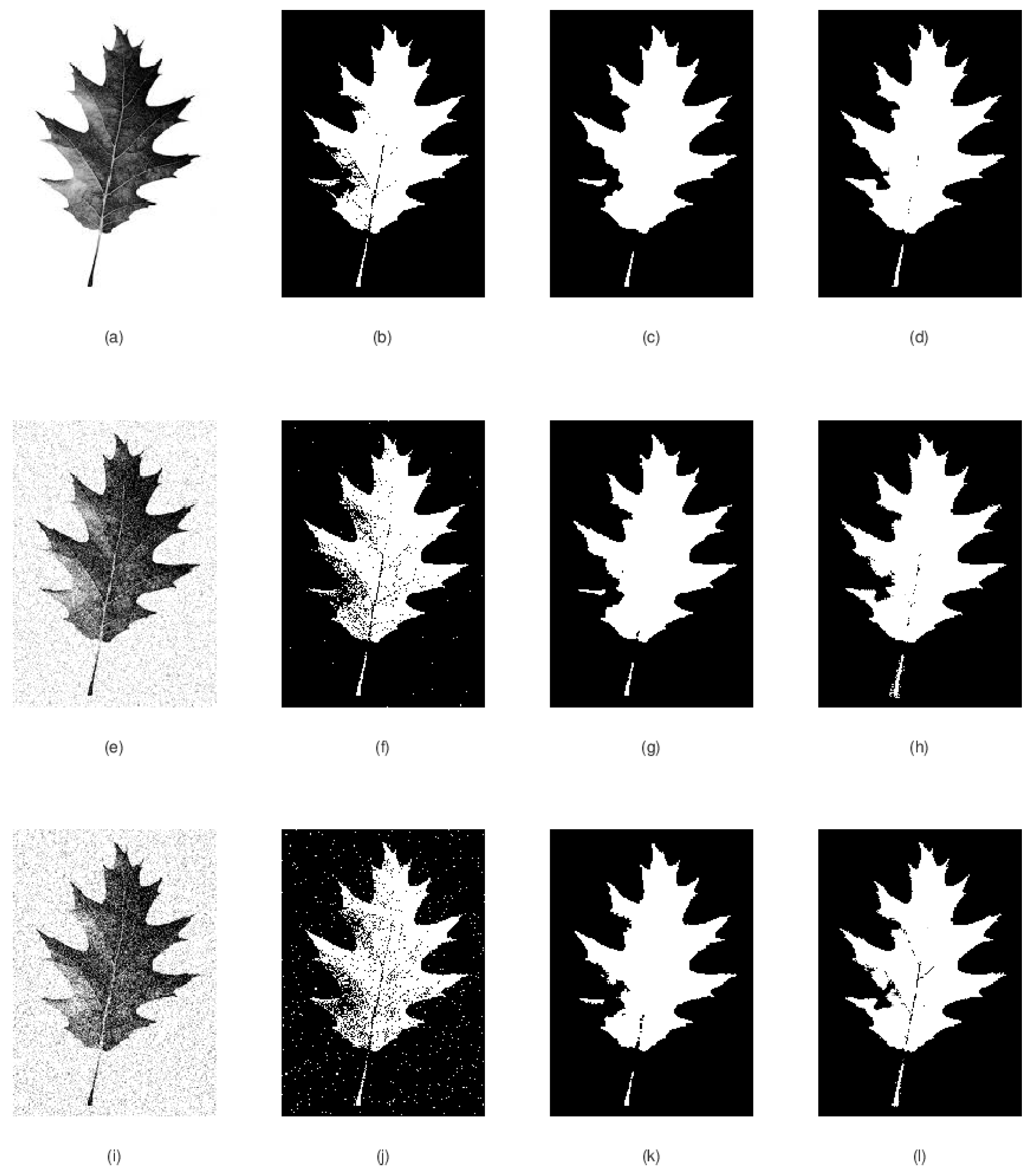
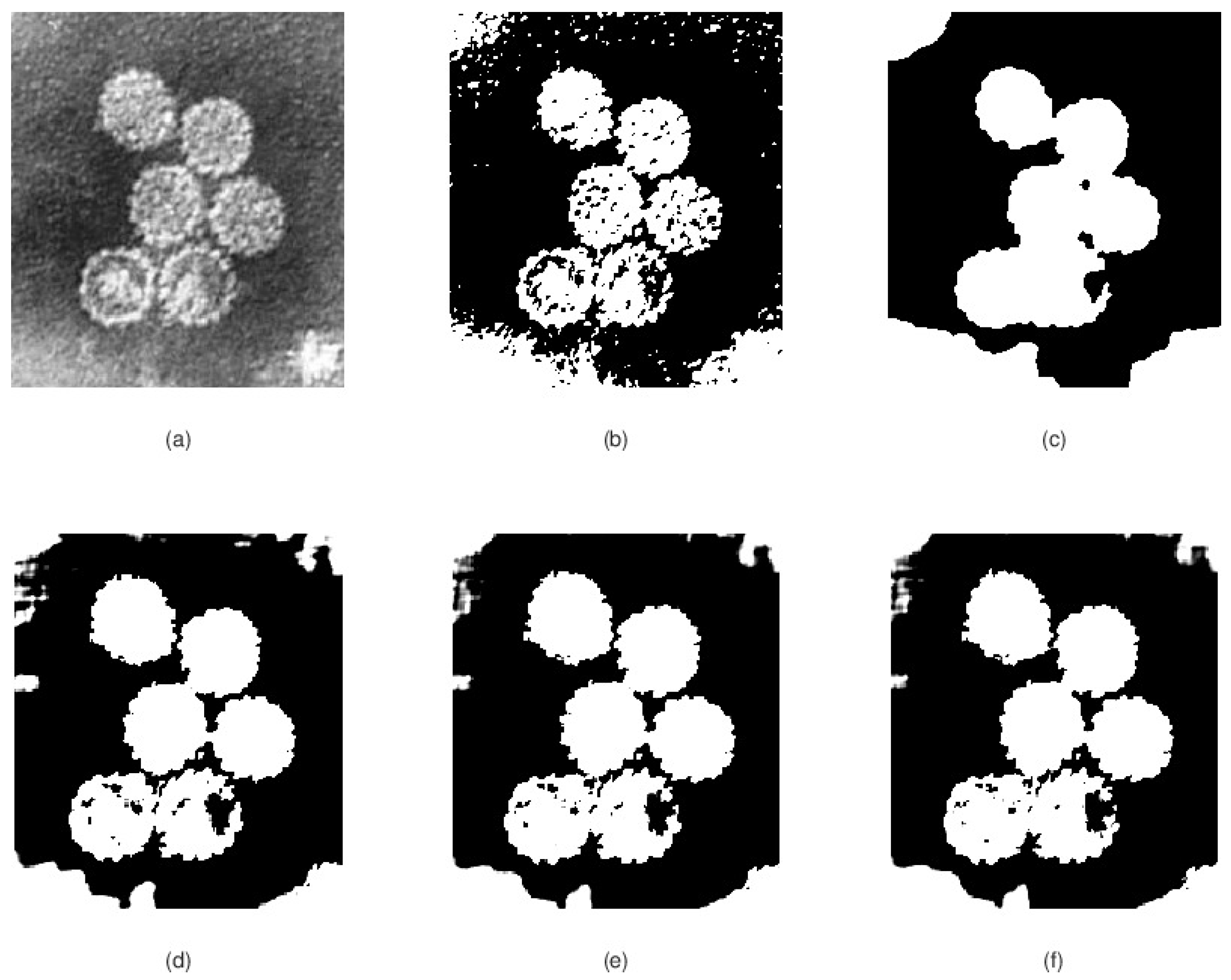
3.2. Experimental Results

The iterative numerical approximation scheme provided by (47) was successfully applied in our image segmentation experiments, for each $m=1,2,\dots ,M-1$, starting with $v^1=v_0\left(x\right)$ (see (33)), which represents the $[Ih\times Jh]$ image to be segmented.

The explicit numerical approximation scheme developed in (47) is consistent to the nonlinear second-order anisotropic reaction–diffusion model given by (32).

In summary, the computations follow the procedure in Algorithm 1. For our tests, we used the following parameter values: $h=1,ϵ=0.1,p_1=0.6,p_3=50,p_4=1,p_5=0.3,\alpha =1,\eta =3$ and $\varphi =1$.

Algorithm 1: Reaction-diffusion based image segmentation algorithm

Some image segmentation results provided by our proposed model are displayed in Figure 1, Figure 2, Figure 3 and Figure 4. All the results presented in this section are compared to standard K-means image segmentation model with two clusters [24] and the Chan–Vese image segmentation model presented in [5].

Our model successfully extracts the objects after up to three iterations. One may see multiple objects as well as objects with boundary concavities and blurry boundaries are accurately extracted from the background.

Figure 1 shows the segmentation results of our model for a brain CT scan image. The results are satisfactory even after only one iteration. We also see the model reaching stability after two iterations in this case. Compared to K-means segmentation results, we observe the extracted objects edges (brain tissue and cranium bone) are better delimited from the background. Compared to Chan–Vese segmentation results, our model produces more accurate results too. In this example, Chan–Vese model seems to not follow the real object boundaries, especially at the border between cranium bone and brain tissue.

Figure 2 shows the segmentation comparison between three cases: first the input image is segmented ‘as is’, second the input image is contaminated with noise before segmentation and third we double the noise added to the input image. For all three cases, we can also see the results of applying K-means and Chan–Vese segmentation. We see our model successfully removes most part of the noise in Figure 2h,l while still preserving a good approximation for the edges on the leaf object (better than both K-means and Chan–Vese).

In Figure 3, we see the segmentation results for a blurry boundary object as galaxy boundaries are slowly fading. Even after one iteration, our segmentation is superior to K-means and Chan–Vese as the real galaxy boundaries are correctly identified in Figure 3d.

Figure 4 (virus microscopy) brings together noise, blur and irregular boundaries. Again, after two iterations, the model successfully identifies all objects of interest and the results, starting with the first iteration, are better than the compared K-means method. The Chan–Vese segmentation does not separate the virus blobs successfully, although it provides a good outer boundary approximation.

Regarding time complexity, due to the integral formulation of $NlD$ term in (41) and (42), the proposed algorithm is slower than the compared K-means or Chan–Vese counterparts. To obtain better performance results, regarding running time, we had to implement the program on parallel architectures such as CUDA [42].

Table 1. Running durations for the reaction-diffusion algorithm implemented on CUDA. The durations are for only one $v^m$ iteration.

Input Area Size (Pixels)	65,536	262,144	1,048,576
Time Taken (Seconds)	0.3	2.0	30.0

shows the time taken by a CUDA implementation for different input image sizes (total number of pixels being $I\ast J$).

Using the local scheme in (48), we obtained promising results for image restoration tasks. Future work will show if we can succeed in mixing the local and nonlocal models for better noise removal before applying segmentation tasks.

4. Conclusions

The starting point in the elaboration of the present work is the paper by Miranville, A. and Moroşanu, C. [1], which is a major challenge for both theory and applications, focused on finding concrete cases of functions for the general case $\mathsf{\Phi }(t,x,v(t,x),v_x(t,x))$ and $\mathsf{\Psi }(t,x,v(t,x),v_x(t,x))$ introduced in [1]. In this respect, a rigorous mathematical investigation is performed to analyze the well-posedness of the nonlinear anisotropic reaction–diffusion model (1) (in particular, (31)). The Leray–Schauder principle is applied to prove the existence and uniqueness of a unique classical solution $v(t,x)\in W_p^{1,2}\left(Q\right)$, while the $L^p$ theory is used to derive the regularity properties for the solutions, considering that the initial data and the boundary constraints are compatible with the regularity and compatibility conditions (see (3)). In addition, the a priori estimates are made in $L^p\left(Q\right)$, which means the approximation for unknown functions $v(t,x)$ are more precise (see [1,11,12,13,15,19,20,21,35]).

Using the finite-difference method (of second-order in time), two numerical schemes are constructed see (47) and (48) to approximate the solution $v(t,x)$ of the new mathematical model. Numerical experiments show the model can be successfully applied to image segmentation tasks. We tested on images with multiple objects as well as objects with complex concavities or blurry boundaries and proved our model can accurately extract them, most of the time showing better results than the compared K-means model.

Summarizing, the main contributions in the present work are as follows:

• We use novel techniques, such as Leray-Schauder principle, a priori estimates, $L^p$-theory, to elaborate a rigorous qualitative study of the nonlocal and nonlinear second-order anisotropic reaction–diffusion parabolic problem, endowed with a nonlinearity of cubic type as well as non-homogeneous Cauchy–Neumann boundary conditions, expressed by (1) and (31). We note that, due to the presence of the nonlinear coefficient $\mathsf{\Phi }(\parallel v_x(t,x))\parallel$ (see (30)), the proposed second-order nonlinear reaction–diffusion scheme (31) represents a non-variational PDE model. Therefore, it cannot be obtained from a minimization of any energy cost functional, thus this scheme is not a variational PDE model.
• Two two numerical schemes (47) and (48) are constructed to approximate the solution of the mathematical models (31) and (32) (local and nonlocal case).

Regarding the second theme, we aim to improve the scheme in (47) and (48), as part of our future research on the topic, by introducing new edge-stopping functions (see [28]) and by taking advantage of non-local image information which will allow us to apply the model to images with inhomogeneity (see [33] and reference therein).

The qualitative results obtained in this current work can be used in quantitative studies of the mathematical models in (1) or (5) as well as in the study of optimal control problems involving such nonlinear problems. We look forward to exploiting all these in our future works.

References

1. Miranville, A.; Moroşanu, C. A Qualitative Analysis of a Nonlinear Second-Order Anisotropic Diffusion Problem with Non-homogeneous Cauchy–Stefan–Boltzmann Boundary Conditions. Appl. Math. Optim. 2019. [Google Scholar] [CrossRef]
2. Allen, S.M.; Cahn, J.W. A microscopic theory for antiphase boundary motion and its application to antiphase domain coarsening. Acta Metall. 1979, 27, 1085–1095. [Google Scholar] [CrossRef]
3. Bates, P.W.; Brown, S.; Han, J. Numerical analysis for a nonlocal Allen-Cahn equation. Int. J. Numer. Anal. Model. 2009, 6, 33–49. [Google Scholar]
4. Bogoya, M.; Gómez, J. On a nonlocal diffusion model with Neumann boundary conditions. Nonlinear Anal. 2012, 75, 3198–3209. [Google Scholar] [CrossRef]
5. Chan, T.F.; Vese, L.A. Active contours without edges. IEEE Trans. Image Process. 2001, 10, 266–277. [Google Scholar] [CrossRef] [Green Version]
6. Caginalp, G.; Lin, J.-T. A numerical analysis of an anisotropic phase field model. IMA J. Appl. Math. 1987, 39, 51–66. [Google Scholar] [CrossRef]
7. Hundsdorfer, W.; Verwer, J. Numerical Solution of Time-Dependent Advection-Diffusion-Reaction Equations; Springer Series in Computational Mathematics; Springer: Berlin/Heidelberg, Germany, 2003; Volume 33. [Google Scholar]
8. de Masi, A.; Orlandi, E.; Presutti, E.; Triolo, L. Stability of the interface in a model of phase separation. Proc. R. Soc. Edin. A 1994, 124, 1013–1022. [Google Scholar] [CrossRef]
9. Moroşanu, C. Approximation of the phase-field transition system via fractional steps method. Numer. Funct. Anal. Optimiz. 1997, 18, 623–648. [Google Scholar] [CrossRef]
10. Moroşanu, C. Cubic spline method and fractional steps schemes to approximate the phase-field system with non-homogeneous Cauchy-Neumann boundary conditions. ROMAI J. 2012, 8, 73–91. [Google Scholar]
11. Moroşanu, C. Analysis and Optimal Control of Phase-Field Transition System: Fractional Steps Methods; Bentham Science Publishers: Sharjah, UAE, 2012. [Google Scholar] [CrossRef] [Green Version]
12. Moroşanu, C. Well-posedness for a phase-field transition system endowed with a polynomial nonlinearity and a general class of nonlinear dynamic boundary conditions. J. Fixed Point Theory Appl. 2016, 18, 225–250. [Google Scholar] [CrossRef]
13. Moroşanu, C. Qualitative and quantitative analysis for a nonlinear reaction-diffusion equation. ROMAI J. 2016, 12, 85–113. Available online: https://rj.romai.ro/arhiva/2016/2/Morosanu.pdf (accessed on 13 December 2020).
14. Moroşanu, C.; Croitoru, A. Analysis of an iterative scheme of fractional steps type associated to the phase-field equation endowed with a general nonlinearity and Cauchy-Neumann boundary conditions. J. Math. Anal. Appl. 2015, 425, 1225–1239. [Google Scholar] [CrossRef]
15. Barbu, T.; Miranville, A.; Moroşanu, C. A qualitative analysis and numerical simulations of a nonlinear second-order anisotropic diffusion problem with non-homogeneous Cauchy-Neumann boundary conditions. Appl. Math. Comput. 2019, 350, 170–180. [Google Scholar] [CrossRef]
16. Moroşanu, C.; Pavăl, S.; Trenchea, C. Analysis of stability and errors of three methods associated to the nonlinear reaction-diffusion equation supplied with homogeneous Neumann boundary conditions. J. Appl. Anal. Comput. 2017, 7, 1–19. [Google Scholar] [CrossRef]
17. Ovono, A.A. Numerical approximation of the phase-field transition system with non-homogeneous Cauchy-Neumann boundary conditions in both unknown functions via fractional steps methods. JAAC 2013, 3, 377–397. [Google Scholar] [CrossRef]
18. Ignat, L.I.; Rossi, J.D. A nonlocal convection-diffusion equation. J. Funct. Anal. 2007, 251, 399–437. [Google Scholar] [CrossRef] [Green Version]
19. Cârjă, O.; Miranville, A.; Moroşanu, C. On the existence, uniqueness and regularity of solutions to the phase-field system with a general regular potential and a general class of nonlinear and non-homogeneous boundary conditions. Nonlinear Anal. TMA 2015, 113, 190–208. [Google Scholar] [CrossRef]
20. Gavriluţ, A.; Moroşanu, C. Well-Posedness for a Nonlinear Reaction-Diffusion Equation Endowed with Nonhomogeneous Cauchy-Neumann Boundary Conditions and Degenerate Mobility. ROMAI J. 2018, 14, 129–141. [Google Scholar]
21. Moroşanu, C.; Motreanu, D. The phase field system with a general nonlinearity. Int. J. Differ. Equ. Appl. 2000, 1, 187–204. [Google Scholar]
22. Gonzalez, R.C.; Woods, R.E.; Eddins, S.L. Digital Image Processing Using Matlab, 2nd ed.; Prentice-Hall: Upper Saddle River, NJ, USA, 2010. [Google Scholar]
23. Jeong, D.; Lee, S.; Lee, D.; Shin, J.; Kim, J. Comparison study of numerical methods for solving the Allen-Cahn equation. Comput. Mater. Sci. 2016, 111, 131–136. [Google Scholar] [CrossRef]
24. Kanungo, T.; Mount, D.M.; Netanyahu, N.S.; Piatko, C.D.; Silverman, R.; Wu, A.Y. An efficient k-means clustering algorithm: Analysis and implementation. IEEE Trans. Pattern Anal. Mach. Intell. 2002, 24, 881–892. [Google Scholar] [CrossRef]
25. Lee, D.; Lee, S. Image Segmentation Based on Modified Fractional Allen–Cahn Equation. Math. Probl. Eng. 2019. [Google Scholar] [CrossRef]
26. Lie, J.; Lysaker, M.; Tai, X.C. A variant of the level set method and applications to image segmentation. Math. Comput. 2006, 75, 1155–1174. [Google Scholar] [CrossRef] [Green Version]
27. Rubinstein, J.; Sternberg, P. Nonlocal reaction-diffusion equations and nucleation. IMA J. Appl. Math. 1992, 48, 249–264. [Google Scholar] [CrossRef]
28. Perona, P.; Malik, J. Scale-space and edge detection using anisotropic diffusion. In Proceedings of the IEEE Computer Society Workshop on Computer Vision, San Juan, PR, USA, 17–19 June 1997; pp. 16–22. [Google Scholar] [CrossRef] [Green Version]
29. Taylor, J.E.; Cahn, J.W. Diffuse interfaces with sharp corners and facets: Phase-field models with strongly anisotropic surfaces. Physics D 1998, 112, 381–411. [Google Scholar] [CrossRef]
30. Weickert, J. Anisotropic Diffusion in Image Processing. In European Consortium for Mathematics in Industry; B. G. Teubner: Stuttgart, Germany, 1998. [Google Scholar]
31. Hu, Y.; Jacob, M. Higher degree total variation (HDTV) regularization for image recovery. IEEE Trans. Image Process. 2012, 21, 2559–2571. [Google Scholar] [CrossRef]
32. Benes, M.; Chalupecky, V.; Mikula, K. Geometrical image segmentation by the Allen–Cahn equation. Appl. Numer. Math. 2004, 51, 187–205. [Google Scholar] [CrossRef]
33. Bresson, X.; Chan, T. Non-Local Unsupervised Variational Image Segmentation Models; Technical Report; UCLA CAM: Los Angeles, CA, USA, 2008; pp. 8–67. [Google Scholar]
34. Cortazar, C.; Elgueta, M.; Rossi, J.D.; Wolanski, N. Boundary fluxes for nonlocal diffusion. J. Differ. Equ. 2007, 234, 360–390. [Google Scholar] [CrossRef] [Green Version]
35. Siddiqi, K.; Lauzière, Y.B.; Tannenbaum, A.; Zucker, S.W. Area and length minimizing flows for shape segmentation. IEEE Trans. Image Process. 1998, 7, 433–443. [Google Scholar] [CrossRef]
36. Tai, X.C.; Christiansen, O.; Lin, P.; Skjælaaen, I. Image segmentation using some piecewise constant level set methods with MBO type of projection. Int. J. Comput. Vis. 2007, 73, 61–76. [Google Scholar] [CrossRef]
37. Vijayakrishna, R.; Kumar, B.V.R.; Halim, A. A PDE Based Image Segmentation Using Fourier Spectral Method. Differ. Equ. Dyn. Syst. 2018. [Google Scholar] [CrossRef]
38. Gilboa, G.; Osher, S. Nonlocal Linear Image Regularization and Supervised Segmentation. Multiscale Model. Simul. 2007, 6, 595–630. [Google Scholar] [CrossRef]
39. Wang, L.-L.; Gu, Y. Efficient Dual Algorithms for Image Segmentation Using TV-Allen-Cahn Type Models. Commun. Comput. Phys. 2011, 9, 859–877. [Google Scholar] [CrossRef]
40. Schonlieb, C.B.; Bertozzi, A. Unconditionally stable schemes for higher order inpainting. Commun. Math. Sci. 2011, 9, 413–457. [Google Scholar]
41. Ruuth, S.J. Implicit-explicit methods for reaction-diffusion problems in pattern formation. J. Math. Biol. 1995, 34, 148–176. [Google Scholar] [CrossRef]
42. Craus, M.; Paval, S.-D. An Accelerating Numerical Computation of the Diffusion Term in a Nonlocal Reaction-Diffusion Equation. Mathematics 2020, 8, 2111. [Google Scholar] [CrossRef]
Figure 1. (a) Original input image to be segmented, (b) K-means segmentation results, (c) Chan–Vese segmentation results; and (df) our model segmentation results after 1–3 iterations, respectively.
Mathematics 09 00091 g001
Figure 2. (a) Original input image to be segmented; (b) K-means segmentation results; (c) Chan–Vese segmentation results; (d) Our model segmentation results after 2 iterations; (e) Input image to be segmented with Gaussian noise added; (f) K-means segmentation results for noisy input in (e); (g) Chan–Vese segmentation results for noisy input in (e); (h) Our model segmentation results for noisy input in (e) after 2 iterations; (i) Input image to be segmented with more noise added; (j) K-means segmentation results for image in (g); (k) Chan–Vese segmentation results for noisy input in (g); and (l) Our model segmentation results for noisy image in (g).
Mathematics 09 00091 g002
Figure 3. (a) Input image to be segmented; (b) K-means segmentation results; (c) Chan–Vese segmentation results; and (df) Our model segmentation results after 1–3 iterations. respectively.
Mathematics 09 00091 g003
Figure 4. (a) Original input image to be segmented; (b) K-means segmentation results; (c) Chan–Vese segmentation results; (df) Our model segmentation results after 1–3 iterations. respectively.
Mathematics 09 00091 g004