In order to complete the definition of the
moea selected for comparison, the crossover, mutation and repair operators must be described. The crossover method aims to uniformly combine a pair of solutions or solutions
I and
to create a new offspring. Given a crossover rate
, which is the probability of applying the operator, and
, all the elements of both solutions will be traversed at the same time, and, for each element
and
, there will be a 50% probability that said elements will be exchanged. The mutation operator is used to randomly replace every gene of a particular solution, i.e., a daily meal consisting of a starter, a main course, and a dessert, with another daily meal with probability
. The repair method is responsible for assessing each solution according to the nutritional value constraints and for determining if the solution is feasible, based on the definition of feasibility given in
Section 3.2. In particular, the same procedure used in the mutation operator will be applied to change a daily meal of a non-feasible solution. The repair operation, however, will be applied always, i.e., no rate is taken into consideration. Each daily meal will be modified by following the aforementioned steps, until a feasible solution is provided.
Experimental method: The Meta-heuristic-based Extensible Tool for Cooperative Optimization (
metco), proposed by León et al. [
52], was used to implement all the algorithms, as well as the
mmpp. Further information about the source code of the
mmpp, the specific instances defined for the current work, and our results can be found at the following
Github repository. The experiments were executed on a
debian
gnu/
linux computer with four
amd®opteron™ processors (model number 6348 HE) at 2.8 GHz with 64 GB of RAM. Unless otherwise specified, each experiment was run 30 times, since all the approaches considered are stochastic. With the aim of statistically comparing the results achieved, the following procedure [
53] was applied. In order to check for the normality of the results, a
Shapiro-Wilk test was applied. Then, if results are normal, a
Levene test is applied to check for homogeneous variances. If results present homogeneous variances, then the
anova test is considered. In the opposite case, the
Welch test is applied. In the case that results do not follow a Gaussian distribution, the
Kruskal–Wallis test is considered. A significance level
is taken into consideration when applying all the above tests.
Ideally, the set of reference points should be the nadir points, i.e., the worst points in the Pareto Front or, in other words, the elements of the Pareto Front that do not dominate any other point. In our case, the worst—maximum—values attained for the two objective functions of the mmpp, considering all the runs performed in each of the experiments, were used to set the reference points. Additionally, the hypervolume was normalized in the range . As we stated before, the higher its value, the better the performance of the algorithm in question.
4.1. First Experiment: Parameter Setting
In this first experiment, we conduct a study involving the values that parameters belonging to the moea selected for comparison should take. Hence, the goal in this first experiment is not focused on comparing the performance of those moea but analyzing their corresponding parameters separately, in order to properly set them for subsequent experiments.
To this end, we tested different values for the parameters of each algorithm, as
Table 3 shows. Specifically, a total of 36 different configurations for each
moea were applied in order to yield a 20-day meal plan. Those configurations were obtained by combining four values for the population size (
n), three values for the mutation rate (
), and three values for the crossover rate (
). In the specific case of parameter
, test values were selected based on the operation of the mutation operator. The reader should recall that a mutation operator specifically designed for the
mmpp is considered herein. Specifically, for each day, the operator modifies the three courses with probability
. Since this experiment requires a 20-day meal plan,
is the minimum probability that allows, at least, one day’s courses to be changed. Bearing the above in mind, the values 0.05, 0.1, and 0.15 were selected; therefore, the courses for one, two, and three days were altered by the mutation operator, respectively. So as to avoid the overly disruptive behavior of the operator, larger values for
were not considered. In the case of the crossover rate, high values are usually set. That is the reason why the test values for parameter
were 0.8, 0.9 and 1.
In order to complement the information given in
Table 3, we should note that all configurations based on the
ibea applied a scaling factor equal to 0.002, while, for each configuration of the
spea2, the archive size was set to the same value considered for the population size. Finally, note that a sufficiently long stopping criterion was set, consisting of
function evaluations. The idea was to study whether the
moea selected converged prematurely or not, and thus determine a proper value for the stopping criterion to be used in subsequent experiments. Furthermore, for this first analysis, and due to the large number of configurations tested, the executions were only repeated 10 times. With respect to the running time of the different approaches, we note that the mean time, considering 10 repetitions of the executions, required by
nsga-ii to perform
function evaluations, was 31,438 seconds, while, in the case of
ibea and
spea2, the mean time was equal to 129,601 and 50,783 seconds, respectively. It can be observed how
nsga-ii is the fastest optimizer, while
ibea is the slowest. The above is probably due to the fact that
ibea needs to calculate a performance metric in order to guide the search, something that is not required by
nsga-ii and
spea2. Anyway, performing a running time analysis of the approaches selected for comparison is out of the scope of the current work.
Table 4 shows some statistical data related to the hypervolume values attained by some configurations of the
nsga-ii at the end of the executions. The reader should recall that 36 different configurations of each
moea were run, but in order to simplify tables, information is only shown for five configurations. Tables including information for the whole set of configurations executed are provided as
Supplementary Material. The last three columns can be used to rank the different configurations tested. In particular, the number of times a given configuration was able to statistically outperform other configurations (
W), and the number of times a particular configuration was statistically outperformed by other configurations (
L) are shown. Configuration
A statistically outperforms configuration
B if the p-value obtained is lower than the significance level
, and, if at the same time,
A provides a higher mean and median for the hypervolume (when the stopping criteria are reached). The ranking (
R) was calculated as the difference between the number of times a configuration outperformed others, and the number of times a configuration was outperformed by others (
). Note that the configurations are shown in descending order based on their position in the ranking as the first criterion, and the mean and the median of the hypervolume as the second and third criteria. With the aim of differentiating the configurations, the nomenclature Algorithm_ps_
n_pm_
_pc_
is used. Finally,
Table 5 and
Table 6 show the same information but for the
ibea and
spea2 approaches, respectively. The same nomenclature is used to differentiate the configurations, but adding some slight modifications to include information on the scaling factor (sFactor) in the case of the
ibea, and the archive size (as) in the case of the
spea2.
With respect to the
nsga-ii, we observed that, in general, larger population sizes yielded better performance in terms of hypervolume values, in comparison to smaller populations. For instance, the values for the first-ranked configuration were
,
, with
solutions, which was the largest population tested. If the same values are set for parameters
and
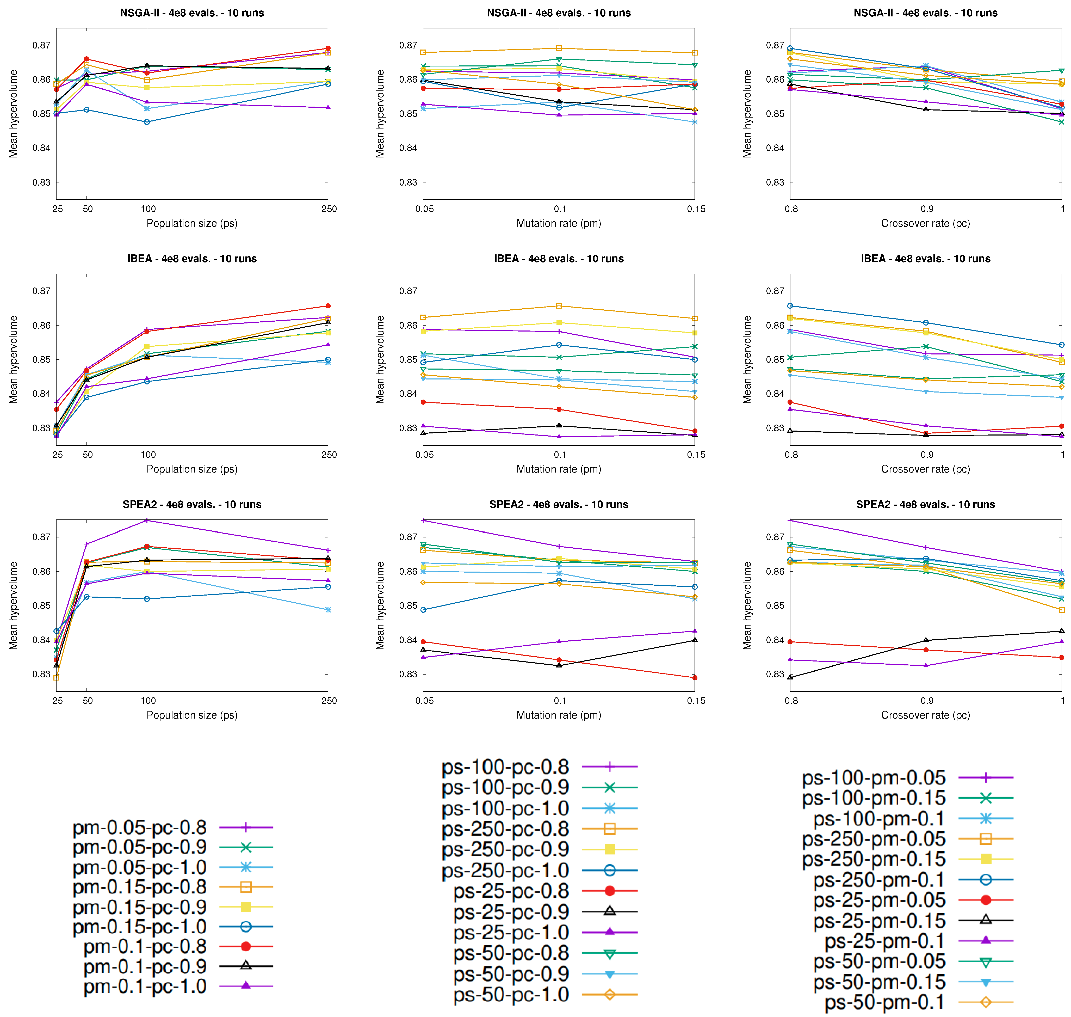
, the worst-ranked configuration contained 25 solutions, which was the smallest population considered. In order to better analyze the above fact,
Figure 3 shows the mean hypervolume values attained by the different configurations of the
nsga-ii (first row), the
ibea (second row), and the
spea2 (third row) at the end of the executions with respect to the population size (first column), the mutation rate (second column), and the crossover rate (third column). In the case of the
nsga-ii, note that, for almost every possible combination of values for parameters
and
(first row, first column), the best results were achieved by applying the largest population considered (
), while the worst results were provided by using the smallest population tested (
).
Regarding the crossover rate, we should note that, generally speaking, lower values yielded better hypervolume values, and therefore better performance, while higher values of the crossover rate decreased the performance of the nsga-ii significantly. As proof of the above, the last five configurations in the ranking were executed with , while, in the first five configurations, .
Moreover, as
Figure 3 shows (first row, third column), in the general case, the lowest hypervolume values were achieved with
, while the highest hypervolume values were attained with
.
In regard to the mutation rate, however, a clear conclusion cannot be extracted. It is true that, for instance, the first three configurations of the
nsga-ii in the ranking had the same population size and crossover rate, with a different value for the mutation rate. Bearing the above in mind, we may claim that the mutation rate
does not seem to have a significant effect on the performance of the
nsga-ii, at least considering the values selected for this study. However, as
Figure 3 shows (first row, second column), in some cases, lower values for the mutation rate provided better results, while higher values of the mutation rate yielded better performance over other cases. As a result, more experiments should be conducted to shed more light on the behavior of the
nsga-ii with respect to the mutation rate, which seems to be its most sensitive parameter when dealing with this particular problem.
Finally, it is important to remark that the first configuration of the nsga-ii in the ranking, which was run with , , and , was able to statistically outperform 28 out of 35 configurations (80%), while it was not statistically outperformed by any other configuration. Furthermore, that configuration achieved the highest mean and median of the hypervolume at the end of the executions, taking into account the 36 different parameterizations of the nsga-ii tested.
Similar conclusions to those given for the
nsga-ii can be extracted for the
ibea (
Table 5 and
Figure 3). In the general case, the application of larger population sizes and lower crossover rates yielded better performance, while the mutation rate seems to be its most sensitive parameter, as in the case of the
nsga-ii. In fact, the configuration of the
ibea that yielded the best performance, i.e., the first configuration in the ranking, was executed with
,
, and
, which was also the best-performing parameterization of the
nsga-ii. The best-performing configuration of the
ibea was able to statistically outperform 32 out of 35 configurations (91.4%), while it was not statistically outperformed by any other configuration. Moreover, we should note that the best-performing configuration of the
ibea achieved the highest median and mean of the hypervolume, considering the 36 different configurations tested, as was the case with the
nsga-ii.
The behavior of the
spea2, however, was slightly different in terms of its parameters (
Table 6 and
Figure 3), and particularly of the population size, with respect to the other two approaches. The best-performing configuration of the
spea2 had
solutions, in contrast to the best-performing configurations of the
nsga-ii and the
ibea, which were run with 250 solutions. The above may be explained by the fact that the
spea2 makes use of an archive in which the size is usually set equal to the value selected for the population size, which allows the non-dominated solutions considered so far to be stored during the executions. The use of that archive may avoid the need to employ larger population sizes. With regard to the remaining parameters (
and
), similar conclusions to those drawn previously for the
nsga-ii and
ibea can be also extracted for the
spea2. Finally, we note that the first configuration of the
spea2 in the ranking statistically outperformed 34 out of 35 configurations (97.1%), while it was not outperformed by any other configuration. As was the case with the
nsga-ii and the
ibea, that first-ranked configuration yielded the highest mean and also median for the hypervolume indicator, considering the 36 different parameterizations of the
spea2.
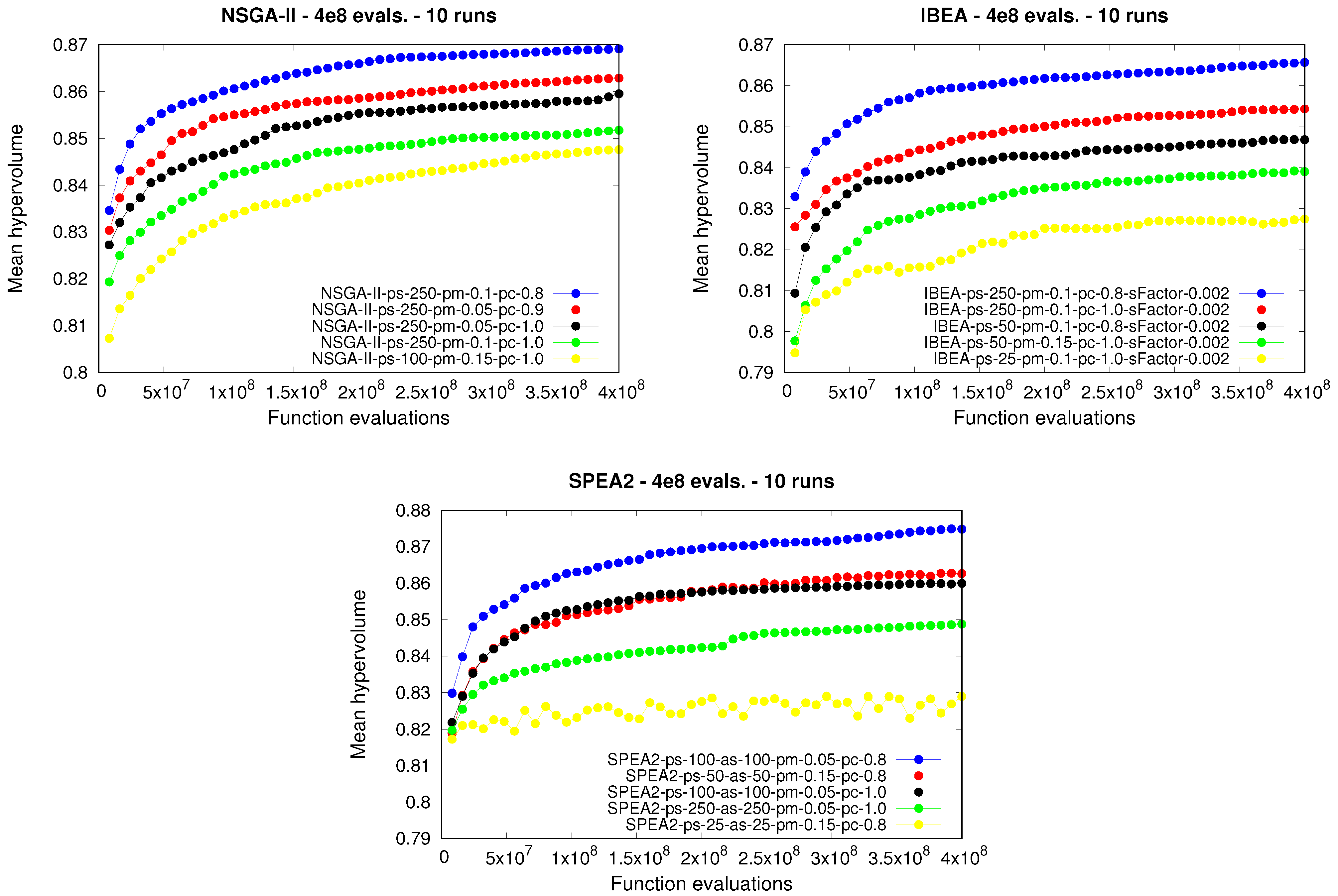
The previous analysis was carried out by considering the results obtained at the end of the executions. However, it would be interesting to study the behavior of the different approaches during the runs. As we said at the beginning of this section, a long stopping criterion was set with the aim of analyzing if any of the
moea selected for comparison converged prematurely.
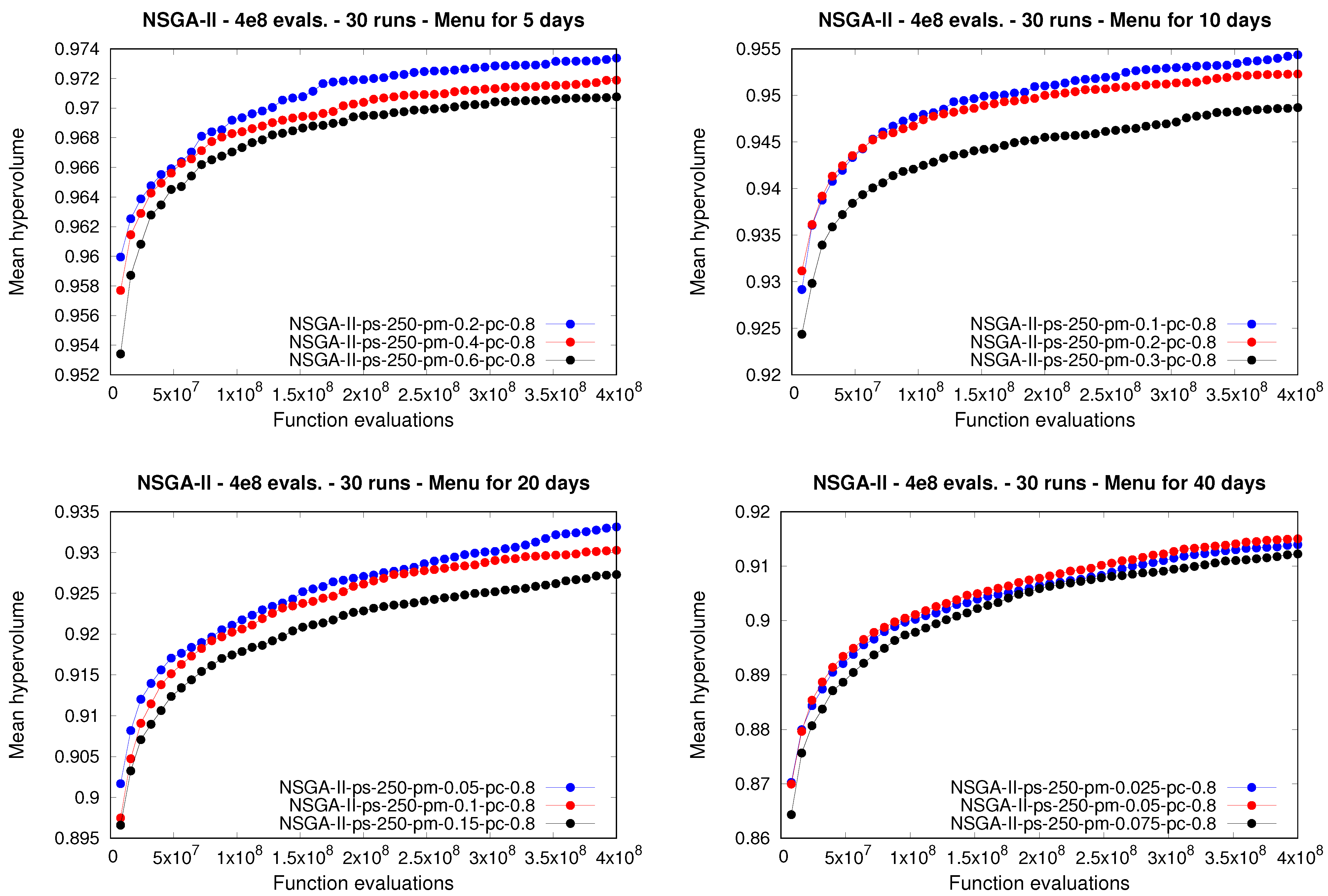
Figure 4 shows the evolution of the mean hypervolume achieved by some configurations of the
nsga-ii, the
ibea and the
spea2. Specifically, for each of the approaches tested, the first and last configurations, i.e., the best- and worst-performing parameterizations, respectively, given their corresponding rankings, were selected for comparison purposes. The configurations ranked 9, 18, and 27 were also included in the comparison. In fact, the above five configurations are those included in
Table 4,
Table 5 and
Table 6. As we can see, for the three approaches, significant differences arose in terms of the performance yielded during the runs by the parameterizations applied, something that we had already stated previously. In addition, despite having set a long stopping criterion consisting of
function evaluations, the mean hypervolume was improved even at the end of the runs, allowing us to conclude that none of the
moea converged prematurely. Bearing the above in mind, runs may be executed for even longer in order to study the behavior of the approaches in the long term.
4.2. Second Experiment: Designing Meal Plans for a Variable Number of Days
The main goal of the second experiment is to analyze the performance of the different moea when they are applied to produce meal plans for a variable number of days. Considering the conclusions extracted from the first experiment, we decided to apply the nsga-ii, ibea, and spea2 with the same parameter values used by their corresponding first-ranked configurations. Hence, the size of the population was set to solutions for nsga-ii and ibea, and to solutions for spea2. The crossover rate was set to for all of the approaches. In addition, the scaling factor of the ibea was set to , and the archive size of the spea2 was set to 100 solutions. Finally, since the first experiment provided no clear conclusions on the mutation rate , three different values were tested in the second experiment for this parameter. Since for this experiment we decided to design meal plans for 5, 10, 20, and 40 days, was set such that the meals for one, two or three days are changed by the mutation operator. For instance, values of , , and were selected when dealing with meal plans for five days, and therefore, the meals for one, two and three days were altered by the mutation operator, respectively. The reader should recall that, in this case, the chromosome would consist of five genes, i.e., the meal plan length, with each gene encoding a starter, a main course, and a dessert. When designing meal plans for 40 days, however, the values , , and were tested.
Bearing the above in mind, three different configurations for each moea were applied to design meal plans for 5, 10, 20, and 40 days. The stopping criterion was also set to function evaluations, as in the first experiment, but this time every run was repeated 30 times rather than 10 times, in an effort to provide much more statistically significant conclusions.
Table 7 shows, for each meal plan length, statistical information related to the hypervolume values provided by each configuration of the different
moea at the end of the runs. The last three columns show data on the statistical ranking achieved by each configuration, which was calculated by following the same procedure explained in the first experiment. Note how, for a small number of days, i.e., 5 and 10 days, the
moea that yielded the best performance at the end of the executions was the
nsga-ii. When designing a meal plan for 5 days, the three highest-ranking configurations were the three parameterizations of the
nsga-ii. In fact, each of those three configurations statistically outperformed every
ibea and
spea2 configuration. When designing a meal plan for 10 days, the three
nsga-ii configurations also obtained the first three positions in the ranking. Although each of its configurations statistically outperformed every
spea2 configuration, some of its configurations did not exhibit statistically significant differences in comparison to some
ibea parameterizations.
For longer meal plans, however, i.e., 20 and 40 days, the best performance at the end of the runs was attained by the spea2. When producing meal plans for 20 days, two configurations of the spea2 where the highest ranked. Those two configurations were able to statistically outperform, or did not exhibit statistically significant differences with respect to, all of the nsga-ii and ibea configurations. Finally, when dealing with 40-day meal plans, the three spea2 configurations obtained the top three positions in the ranking, with each of them statistically outperforming each nsga-ii and ibea configuration.
Regarding the mutation rate, note how small values yielded better performance in comparison to larger ones. In fact, when designing meal plans for 5 and 10 days, where the nsga-ii was the best-performing moea, those configurations that used the smallest mutation rate tested obtained the first position in their corresponding rankings. When dealing with longer meal plans, i.e., for 20 and 40 days, the spea2 behaved similarly, with lower mutation rates providing better performance in comparison to higher values of this parameter.
As was done in the first experiment, it is interesting to study the behavior of the
moea both during and at the end of the executions.
Figure 5 shows, for each meal plan length considered in this experiment, the evolution of the mean hypervolume attained by the
nsga-ii.
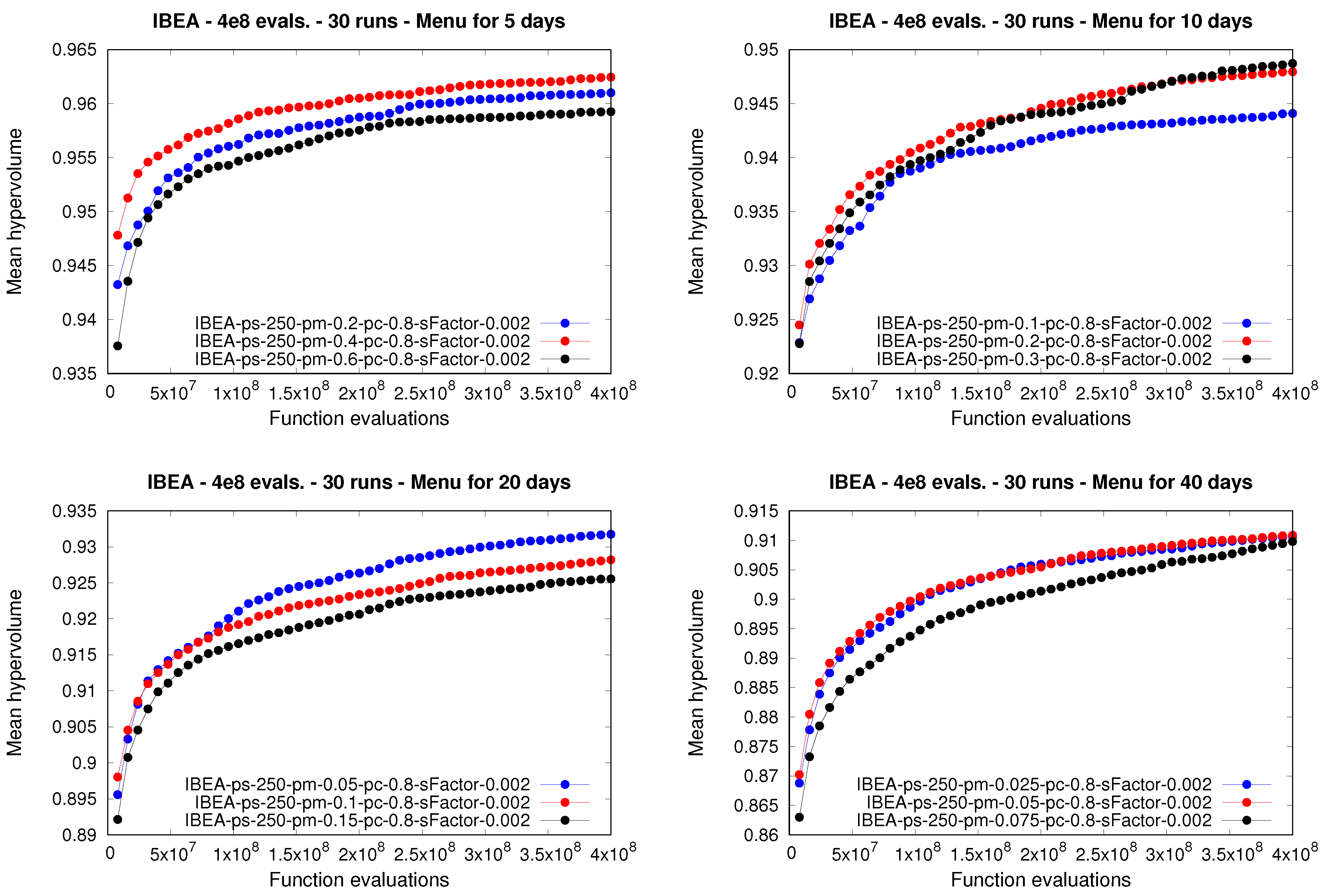
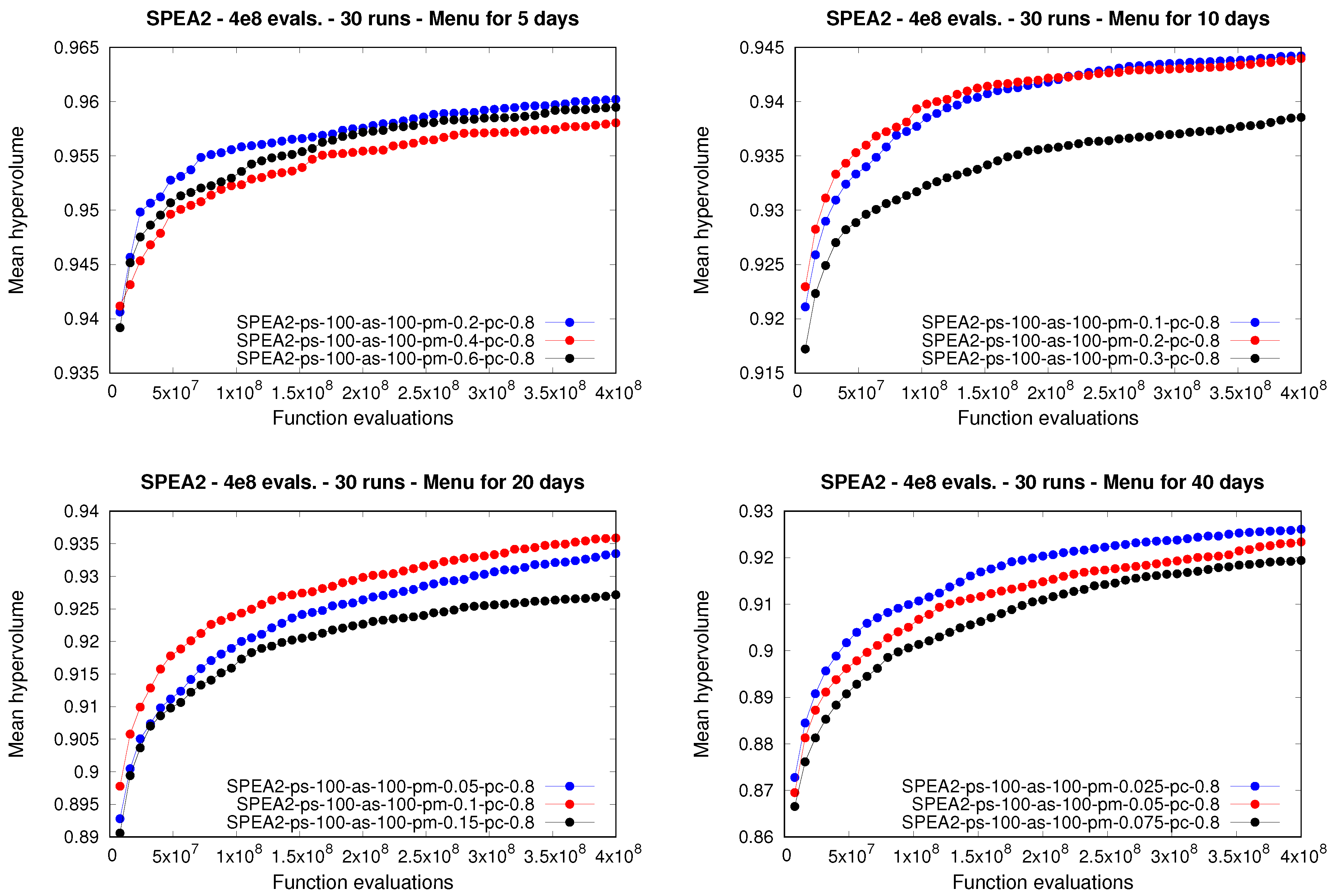
Figure 6 and
Figure 7 show the same information for the
ibea and the
spea2, respectively. Note how the three
moea exhibited differences during the runs depending on the specific value selected for the mutation rate. Although a few exceptions arose for some instances, particularly in the case of the
ibea, in general, every approach that used lower values for the mutation rate was able to attain a higher mean for the hypervolume, and therefore better performance, during almost every execution, in comparison to using larger mutation rates.
4.3. Third Experiment: Qualitative and Quantitative Analysis of Solutions
In this third experiment, the main goal is to analyze the solutions attained by the moea considered in this paper from both a quantitative and qualitative point of view. Additionally, we would like to validate the multi-objective formulation of the mpp we are providing herein in terms of the features of the solutions achieved. In order to do this, we considered, for each meal plan length, the solutions obtained in the second experiment by the best- and worst-performing configurations of each moea, i.e., the configurations obtaining the first and last positions in their corresponding ranking.
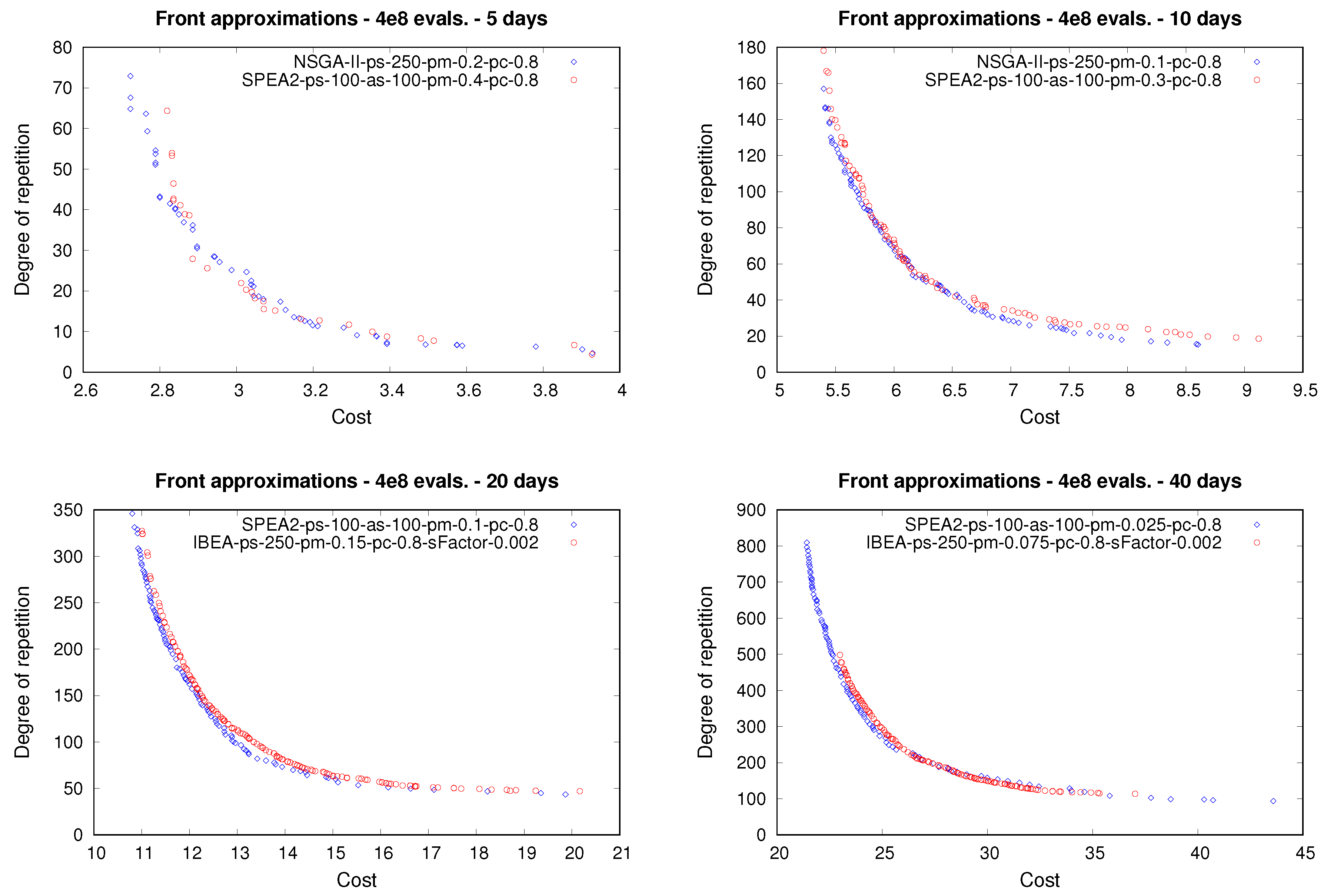
Figure 8 shows, for each meal plan length, examples of front approximations obtained after the tests by those best- and worst-performing parameterizations. First of all, we should note that the shape of the different front approximations obtained demonstrates that the two objective functions are in conflict with each other. A decrease in the cost of a meal plan entails an increase in the frequency of course repetitions, and vice-versa. Bearing the above in mind, we can state that the multi-objective formulation of the
mpp we are proposing herein is valid from the standpoint of its multi-objective nature.
Note also that differences among the front approximations attained by the best-performing and worst-performing configurations arose for each plan length. Generally speaking, for each case, the best-performing configuration was able to provide a better front approximation not only in terms of its convergence but also in terms of its spread and uniformity, features that are closely related to each other and that are usually referred to as the diversity of a front. For instance, when dealing with meal plans for 10 and 20 days, it holds that the corresponding best-performing configuration is able to provide a significant number of solutions that dominate a large number of solutions attained by the corresponding worst-performing configuration. The improvement in performance provided by the best configuration with respect to the worst one was even more noticeable when designing 40-day meal plans. The best-performing configuration was able to provide solutions located in regions of the front that are not covered by those solutions attained by the worst-performing configuration. It can be observed that in the case of smaller instances, the best-performing approach was nsga-ii, while, in the case of larger instances, the best-performing scheme was spea2. It is important to recall that one of the main differences of spea2 in comparison to nsga-ii and ibea is that the former makes use of an archive, which allows the non-dominated solutions achieved so far to be stored during the executions. The use of an archive could have a significant impact over the performance of an optimizer when dealing with larger instances. Nevertheless, more experiments are required to clarify the above.
Finally, it would also be interesting to analyze one of those solutions in depth, not only from the point of view of the different meals that it offers but also from the point of view of its nutritional value. In order to do that, we selected one of the 10-day meal plans obtained by the corresponding best-performing configuration for which the values for the cost and the degree of repetition were
and
, respectively.
Table 8 enumerates the different meals in said meal plan, while
Table 9 describes the total amount of nutrients it provides. According to the White Book on Child Nutrition, the main nutrients to consider in the case of lunch are carbohydrates, fats and proteins. The total number of kilocalories recommended for a child is 2000 kcal per day. Lunch accounts for approximately 35% of the total daily nutrient intake. As a result, the recommended number of kilocalories in a lunch should be approximately 700 kcal. The meal plan depicted in
Table 8 contains a total of 7269.34 kcal, which provides the recommended kilocalorie intake for 10.4 days. Regarding the total recommended amount of fats, they should contribute no more than 35% of the total amount of energy, meaning that, for a lunch of 700 kcal, 245 kcal should come from fats. One gram of fat provides 9 kcal, so one lunch should contain 27.2 g of fat. The 10-day meal plan in our example provides 282.05 g of fat, which corresponds to the total amount of fats for 10.4 days. The recommended amount of carbohydrates is 50% of the total energy intake provided by one lunch; consequently, 350 kcal should come from carbohydrates. One gram of carbohydrate provides 4 kcal, and, as a result, a lunch should contain 87.5 g of carbohydrates. Our meal plan provides 769.24 g of carbohydrates, which corresponds to the total amount for 8.8 days. Finally, the recommended amount of proteins is 15% of the total energy provided by one lunch, which means that 105 kcal should come from proteins. One gram of protein provides 4 kcal; therefore, a lunch should contain 26.25 g of protein. Our meal plan example provides 291.08 g of proteins, which is equivalent to 11.1 days in terms of the intake recommendation. In conclusion, although the recommended amounts of nutrients may vary slightly from one recommendation to the next, and in practical terms there is a margin of excess and deficiency of nutrients above and below the recommended amounts, the meal plan selected for this study provides, in general terms, an adequate and balanced amount of nutrients.

 ,
, 


