Chemical Graph Theory for Property Modeling in QSAR and QSPR—Charming QSAR & QSPR

Abstract

Quantitative structure-activity relationship (QSAR) and Quantitative structure-property relationship (QSPR) are mathematical models for the prediction of the chemical, physical or biological properties of chemical compounds. Usually, they are based on structural (grounded on fragment contribution) or calculated (centered on QSAR three-dimensional (QSAR-3D) or chemical descriptors) parameters. Hereby, we describe a Graph Theory approach for generating and mining molecular fragments to be used in QSAR or QSPR modeling based exclusively on fragment contributions. Merging of Molecular Graph Theory, Simplified Molecular Input Line Entry Specification (SMILES) notation, and the connection table data allows a precise way to differentiate and count the molecular fragments. Machine learning strategies generated models with outstanding root mean square error (RMSE) and R² values. We also present the software Charming QSAR & QSPR, written in Python, for the property prediction of chemical compounds while using this approach.

1. Introduction

Quantitative structure-activity relationship (QSAR) and Quantitative structure-property relationship (QSPR) correlate structural parameters with a determinate attribute while using statistical tools. In principle, any complex characteristic can be modeled by QSAR or QSPR, such as toxicity, IC₅₀, cetane number, solubility, and so on. Despite the studied property being reported as a single number, it is already influenced by several physicochemical parameters that also depend on the molecular structure [1]. The observed biological activity, for example, relates to specific intermolecular interactions, membrane permeability, pKa, molecular weight, polarity, and a dozen more characteristics. Eventually, some of those traits may act synergistically in order to improve the observed result, but others, instead, behave antagonistically [1,2,3,4,5,6,7,8,9].

QSAR and QSPR work with structural, experimental, or theoretical parameters in order to model a specific property, usually using a weighted composition of them. When considering that any property ultimately arises from the connection pattern, geometry, and the molecular structure if the number of compounds in the study set is large enough and the structural parameters are sufficiently precise, it is possible to anticipate any desired property while using exclusively the structural data of the study set [2,3,4,5,6,7,8,9]. This work presents a software that was developed by our group that exclusively uses the chemical graph theory to generate a small set of molecular fragments that were obtained from the original study set to model a specific property.

A molecular property can be interpreted as a summoning of positive and negative contributions of different fragments in the compound. Polar groups, for example, interact among them and increase the boiling point of a substance. The molecular symmetry and polarity of a molecule may facilitate intermolecular interactions and increase its melting point. The biological activity of a small molecule is a result of specific interactions between the compound and a macromolecular target. In this case, such molecular recognition arises from pharmacophoric interaction points into the active site. All of those molecular properties evolve from increments of positive and negative contributions of the different substructural fragments in the whole molecule [2,3,4,5,6,7,8,9]. In this way, substructural descriptors are already used in QSAR/QSPR studies and their counts help to quantify the desired property, and they are readily calculable from the molecular structure.

Graph theory concepts are present in our daily routine, although we do not perceive it. Situations, such as routing internet traffic, finding the shortest path between two points, and map coloring, are typical examples. Conversely, in chemistry, those concepts can be found in HMO, protein folding, and nomenclature, just to cite a few cases [1,10].

There is a great resemblance between a graph and structural formula, as depicted in Figure 1, in which a direct correlation among vertices and atoms, as well as edges and chemical bonds, is clearly perceived. Unfortunately, a critical drawback precludes a more generalized use of the graph theory in chemistry—the incapability to distinguish atoms or bonds [11,12,13,14,15,16,17,18,19,20,21,22].

The quantification of specific interactions among substructural fragments is crucial to infer any molecular property and, to do so, it is crucial to differentiate atoms and chemical bonds, as stated previously. In order to circumvent the above-mentioned weakness of graph theory, we envisage its simultaneous use with the SMILES linear notation of chemical structures [23,24]. It is relatively fast and precise to determine all of the subgraphs in a more complex graph using the graphs theory. The inability to differentiate atoms or bonds on the graph theory is thwarted while using SMILES through the correspondence of each substructural fragment that was obtained from the graph theory with the atom connection pattern obtained from the input data. Structural chemical data, such as a mol file or similar, define different types of chemical bonds that are used to connect different atoms and such information is transferred precisely to the SMILES notation [17,18,19,20,21,22,23,24]. While using such an approach, it is possible to discriminate any atom, even its hybridization, as well as its precise location into the molecule. Thereby, it would be possible to tell whether an oxygen atom is an alcohol, ether, or ester group, for example. Figure 1 shows an example of the aforesaid approach, which was used in the Charming QSAR & QSPR software described here. Applying this approach, a graph is built using the connectivity information from the input data. Accordingly, each subgraph obtained by the graph theory corresponds to a substructural fragment, which is notated in SMILES, retrieving the corresponding chemical information.

In Charming QSAR & QSPR, the activity model is achieved from a multivariate linear regression while using molecular fragment frequencies as descriptors. The frequency is simply calculated by counting the number of occurrences of an independent molecular fragment that is produced by the Graph Theory/SMILES/Structural Data approach described above.

2. Methods

2.1. The Charming QSPR & QSPR

The Charming QSPR & QSPR program is concerned about mining molecular fragments and generating predictive QSAR models that enlighten the main structural patterns that are related to a given property of a molecule set. The program is written in Python and it uses several RDKit tools, such as SDWriter, MolToSmiles, and MolFragmentToSmiles [25]. It also uses Scikit-learn tools for model selection, statistical metrics, regressions, and machine learning [26]. The input data have SDF file format, and each compound is handled at a time. The applied sequence (Figure 1) begins with the conversion of the input molecule into a benchmarked molecular coordinate while using Chem.SDMolSupplier. The tool follows the required steps to generate and validate a QSAR model, and they are listed below.

2.2. Standardization

Standardization is an important step for building a QSAR model that permits the removal of inconsistent and duplicated data that, otherwise, can input an error at the model elaboration. For standardization, the Charming QSAR & QSPR has a function, builds using the functionalities of the RDKit, called standardized_molecules that accepts an SDF file as input, and searches for duplicates on the work set. This function uses the tautomer enumerator and standardization functionalities of the RDKit Chem module in order to create a standard representation and SMILES nomenclature to compare different structures on the SDF file [23,24,26]. It also sets upper and down limits to molecular mass and a maximum number to each halogen atom.

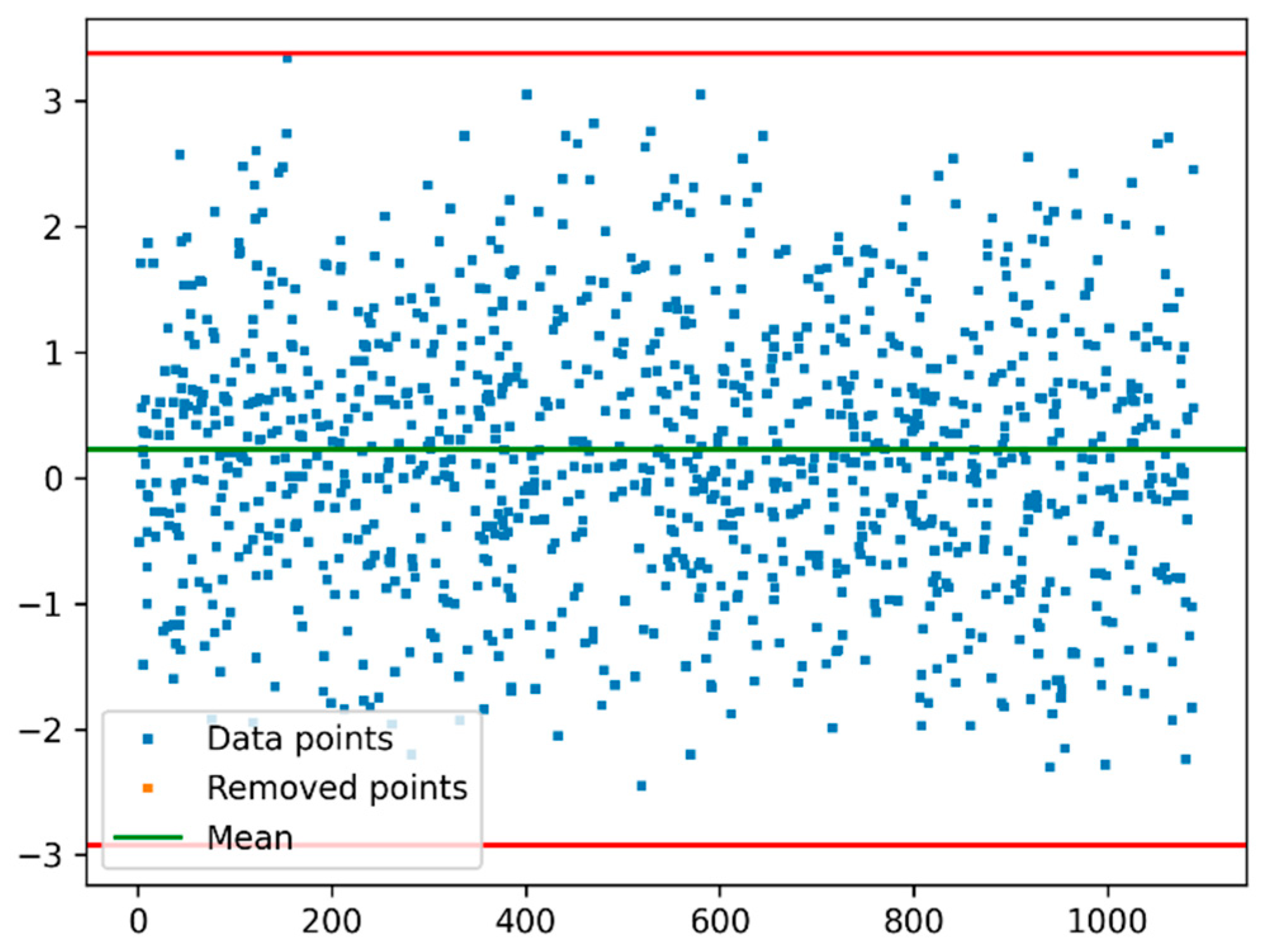
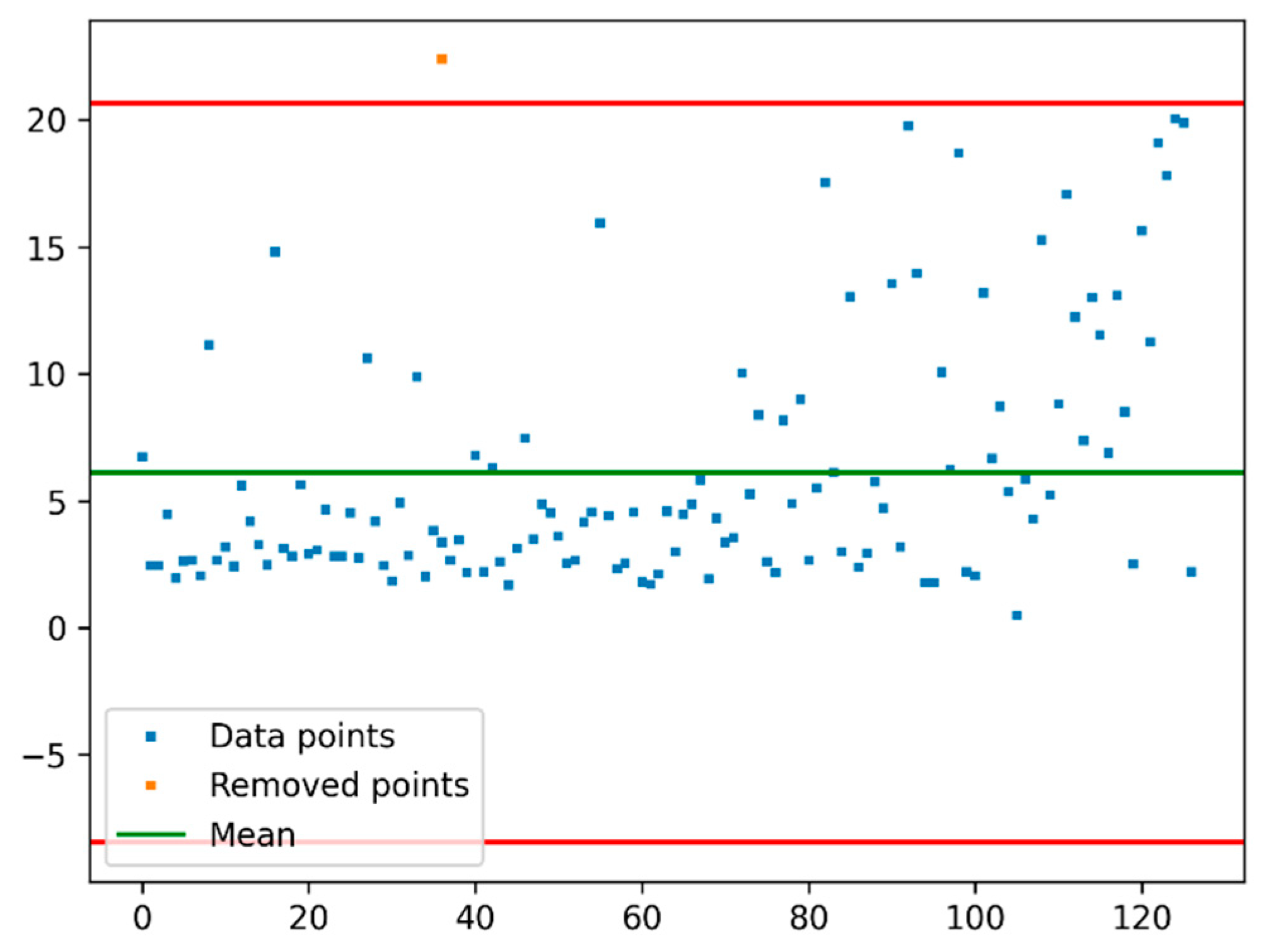
2.3. Outliers

The package that is presented here displays a functionality to identify possible outliers on the endpoint of the work set compounds. This tool is called rem_poss_out, which calculates the average of endpoints values. Based on the standard deviation, it removes the possible outliers. The cut-off value for finding outliers was Z-scores of ±3. The outlying is necessary when some molecules have unexpected or different biological/chemical/physical activity contributing to the endpoint. In such cases, the outlined compounds do not fit in a QSAR model, because such compounds may be acting in a different mechanism of action, having a different target biomolecule [27] or having different binding modes due to conformational flexibility [28]. The input data are the standardized SDF file, and the outputs are the endpoint’s scatter plot and two SDF files, one with the removed compounds and the second with the selected ones.

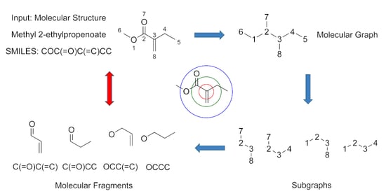
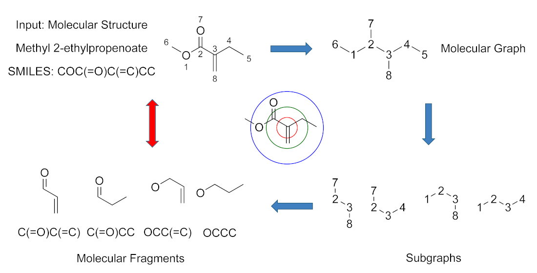
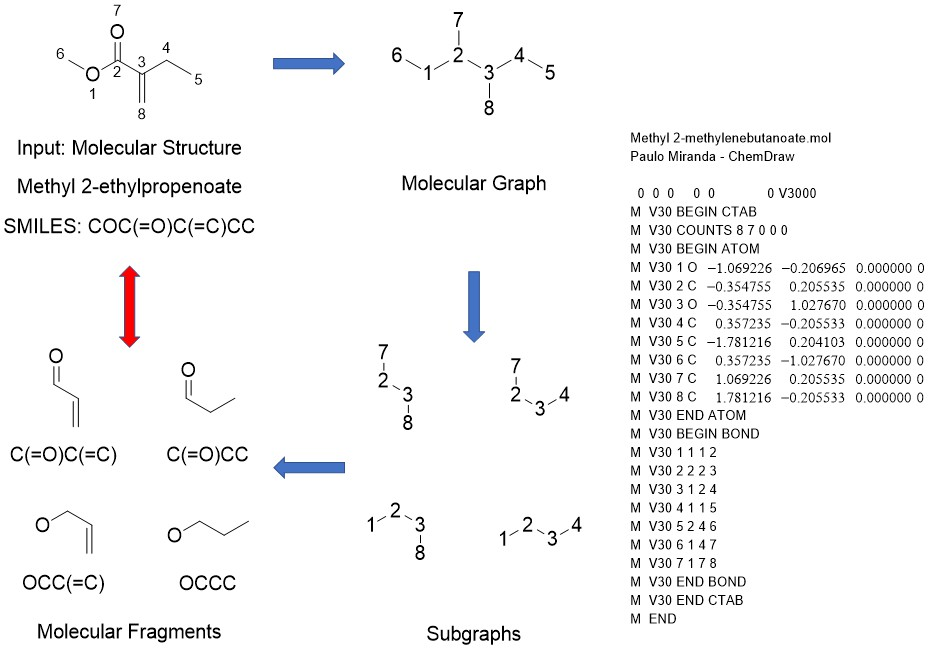
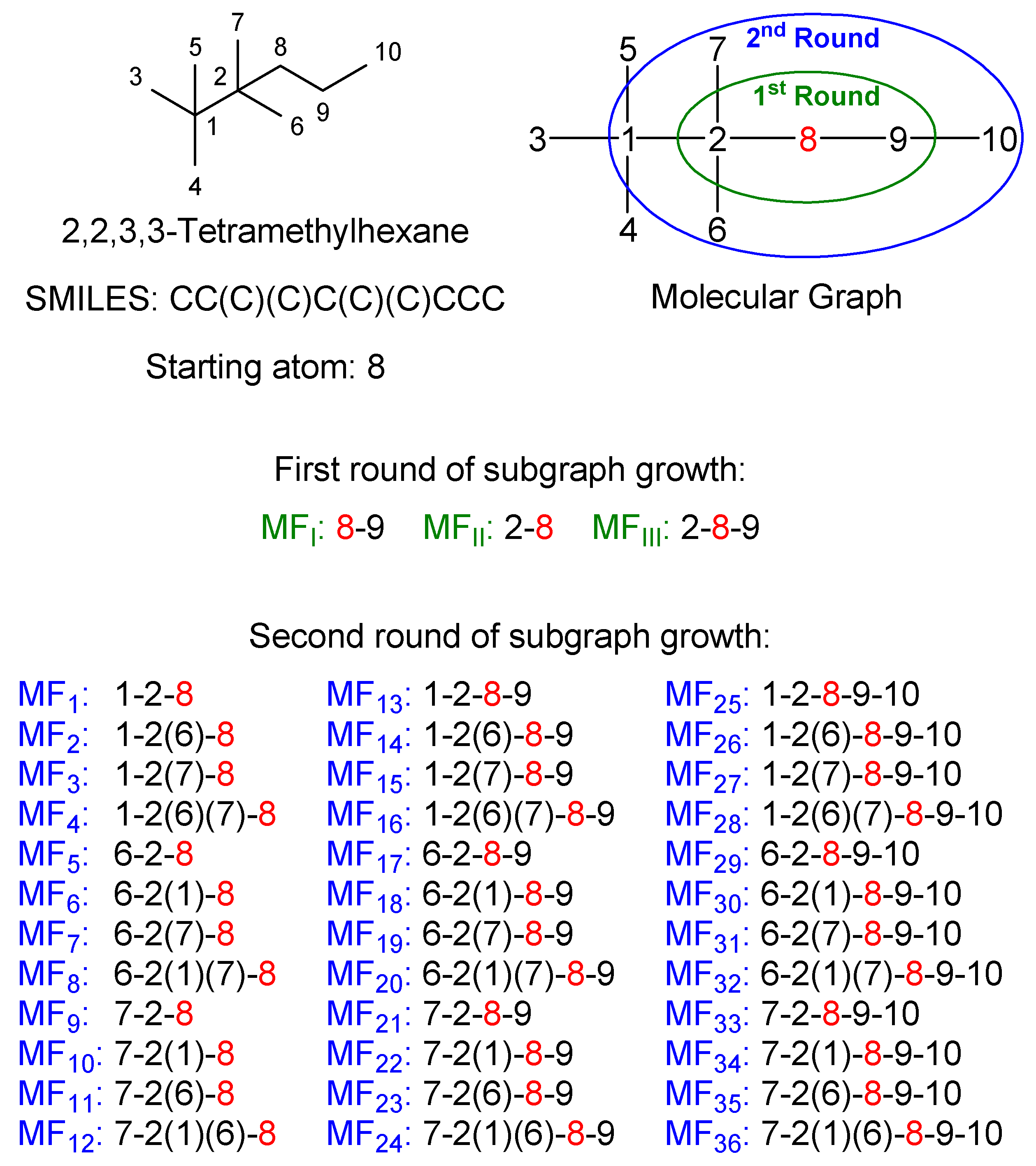
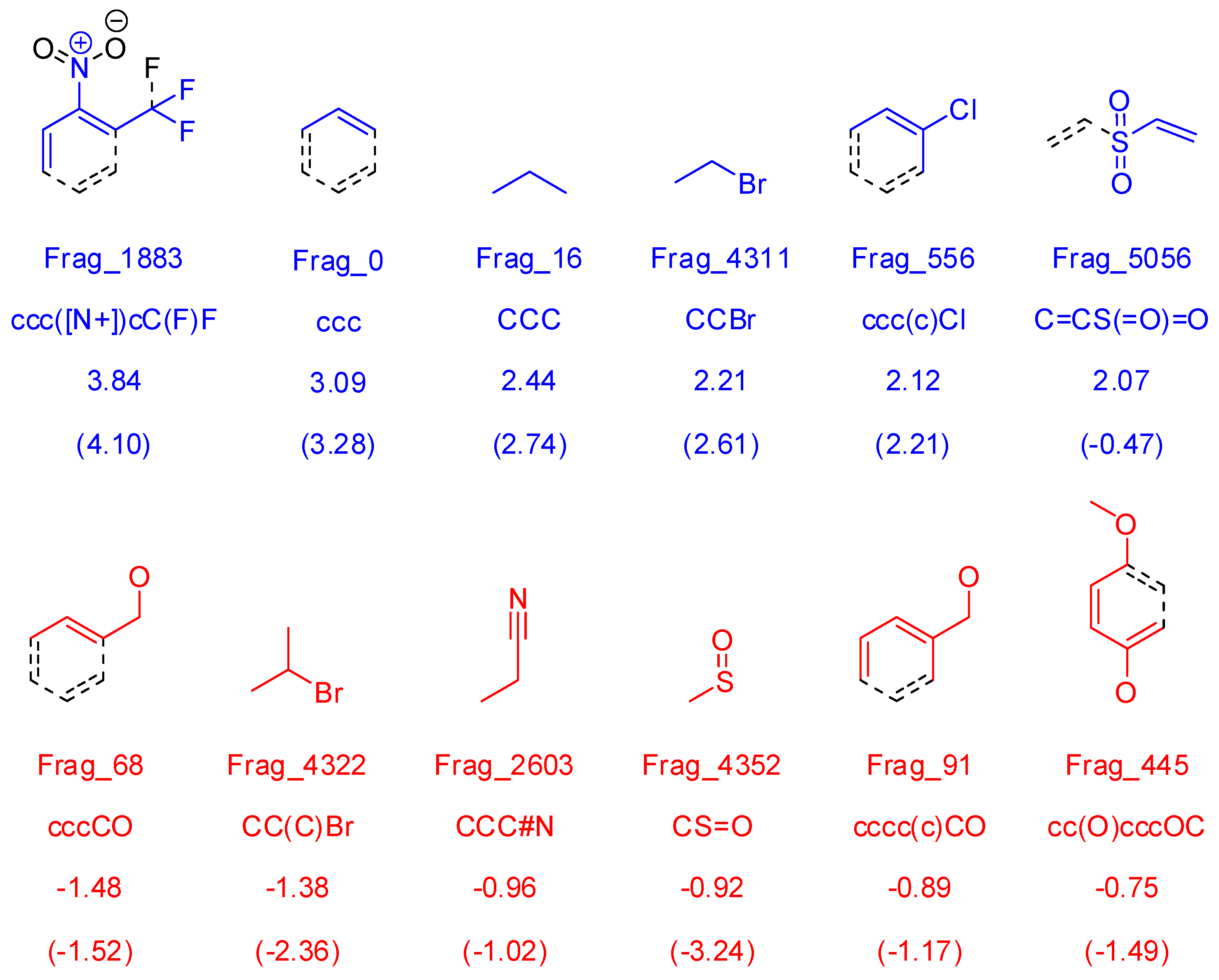
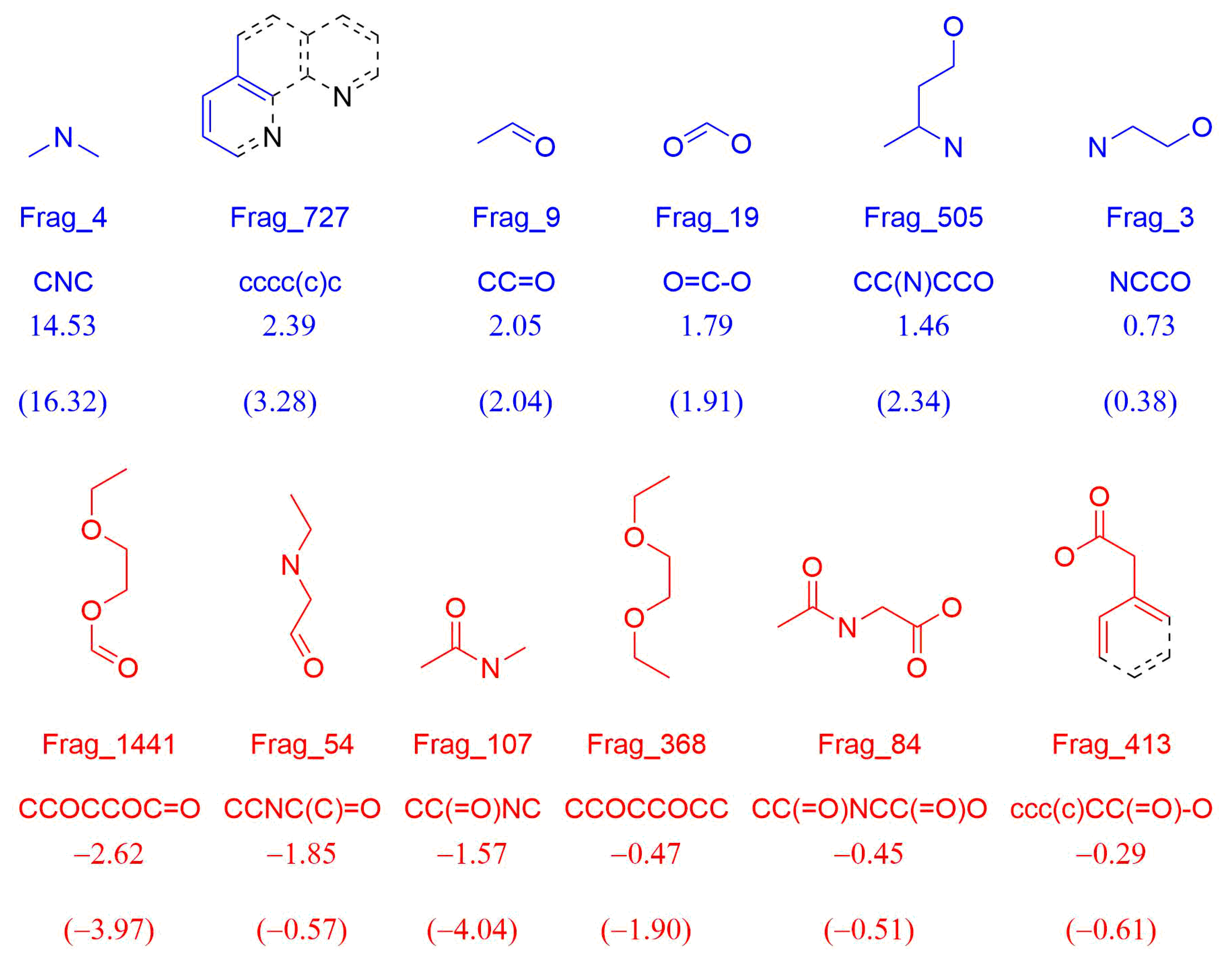
2.4. Molecular Fragment Generation and Counting

The molecular fragments (MF) are the descriptors that are used to portray the compounds set. The package has a function that generates MFs within the range of lengths that are arbitrated by the user. The sequential addition of edges to an empty graph engenders a molecular graph. Each edge is denoted by two connected vertices that, in this case, represent two bonded atoms. After the addition of all edges (bonds) of a compound structure, the molecular graph is submitted to subgraph mining that returns straight and branched paths.

In order to engender the subgraphs, an atom is selected, and its neighbors are added, one at a time, according to the connecting pattern. All of the possible combinations of neighboring atoms are calculated and registered, as depicted in Figure 2. Subsequently, each neighbor in each generated combination is the starting point for the next round of growth. The growth step is repeated until the graph reaches the maximum limit of atoms. The subgraphs that fulfill the requirements that are established by the user are recorded in its SMILES notation. The function repeats this process for each atom in a molecule and each molecule in the SDF file. After that, the duplicated MFs are removed, and their SMILES strings are saved into a CSV file. The correlation table is constructed by accounting for the matching of each MF at all molecular structures. The SMILES notation is also used by the CORAL software [29,30,31] in order to calculate the descriptors, and molecular graphs to calculate the local graph invariants. Conversely, Charming uses the graph theory as a tool for structural patterns engendering. Each generated subgraph is stored, and the SMILES notation is used in order to codify its chemical information.

2.5. Preprocessing

The work set is randomly split into training and test sets containing, typically, 80% for the training set and 20% for the test set. Subsequently, the descriptors (MF) pass through two filter functions: the first is related to the variance and it has a minimum variance threshold; the second analyses the correlation among the descriptors, where the highly correlated MFs are removed. Two or more MF are considered to be correlated when a graph MF₁ is a subgraph of MF₂ and they have a linear dependency. The fragments considered rare was removed. The fragments are considered to be rare if they are present on less than a minimum number of molecules on the training set; this value is set when observing the length of the training set. After that, a study with the most appropriate correlation threshold was performed. Among the values of 0.99, 0.95, and 0.90, the value of 0.99 has the best performance at the machine learning model elaboration. At the end of the whole process, the table with the counting of all MF has all of the descriptors’ range scaled between 0 and 1. This process furnishes a learning algorithm with all equally weighted inputs and then removes the repeated information.

2.6. Descriptor Selection

It is necessary to select the best set of descriptors that are most correlated with the studied property in order to avoid overfitting. For description selection, the Charming QSAR & QSPR has a tool with a backward selection function that selects the descriptors with the p value being adjusted to a multilinear regression. The use of this tool is indicated in small datasets where the number of descriptors is reduced.

The LASSO regression (Least Absolute Shrinkage and Selection Operator) can also be applied to select the descriptors; it is a linear model that calculates sparse coefficients; in other words, it prefers solutions with fewer non-zero coefficients, reducing the dimensionality of the data [32,33,34].

The Random Forest (RF) regressor can also be used to select the MF, and its performance was evaluated in each case studied here. Invariably, in the case of the three examples presented in this work, the descriptors that were selected by LASSO model showed a better description of the chemical space.

2.7. Model Training

The Scikit-learn has several machine learning algorithms, and three of them were selected: support vector machine (SVM), random forest (RF), and gradient boosting machine (GBM) [26]. Only the descriptors with nonzero coefficients at the LASSO model are used to describe the studied property. For each machine learning algorithm, a grid for hyperparameter optimization is used and the best training model is selected. A linear stacking and ensemble of the training models is performed in order to improve the prediction accuracy. After each training process, the test set is used in order to verify the model quality and predictive power.

2.8. Validation

Some statistic metrics are observed to verify the accuracy and predictive ability of the model. The root mean square error (RMSE) is the most appropriate among them. This metric is considered during both steps: model elaboration and validation [35,36,37]. It is defined as:

$$\mathrm{RMSE}= \sqrt{\frac{{\left(y_j- {\tilde{y}}_j\right)}^2}{N}}$$

(1)

where $y_j$ is the property value, ${\tilde{y}}_j$ is the predicted value, and N is the number of molecules in the set.

During the model elaboration, R² is also considered:

$$R_{tr}^2 =1- \frac{{\sum }_{i=1}^{N_{tr}}{(y_i- {\tilde{y}}_i)}^2}{{\sum }_{i=1}^{N_{tr}}{(y_i- {\overline{y}}_{tr})}^2}$$

(2)

where $N_{tr}$ is the number of compounds in the training set, $y_j$ is the experimental value, ${\tilde{y}}_j$ is the predicted value, and ${\overline{y}}_{tr}$ is the average value for the studied property in the training set [35,36,37].

During the test step, in addition to RMSE, the $R^2$ and $R_0^2$ are also considered, defined as:

$$R_{test}= \frac{{\sum }_{j=1}^{N_{test}}(y_j- {\overline{y}}_{test})\left({\tilde{y}}_j - {\overline{\tilde{y}}}_{test} \right)}{\sqrt{{\sum }_{j=1}^{N_{test}}{(y_j- {\overline{y}}_{test})}^2{\left({\tilde{y}}_j - {\overline{\tilde{y}}}_{test}\right)}^2}}$$

(3)

$$R_{0 test}^2= 1-\frac{{\sum }_{j=1}^{N_{test}}{\left(y_j-{\tilde{y}}_j^{r0}\right)}^2}{{\sum }_{j=1}^{N_{test}}{\left(y_j-{\overline{y}}_{test}\right)}^2}$$

(4)

where $N_{test}$ is the number of entries at the test set, $y_j$ is the experimental value, ${\tilde{y}}_j$ is the predicted value, the ${\overline{y}}_{test}$ is the average value for the studied property on the test set, and ${\overline{\tilde{y}}}_{test}$ is the mean of the predicted value. $R_{0 test}^2$ is the coefficient of determination of a regression that has no linear coefficient: ${\tilde{y}}_j^{r0}=k{\tilde{y}}_j$ [35,36,37].

The observed value of the referred metrics permits the analysis of the model performance according to the procedure that was proposed by Tropsha and Golbraikh. In this way, the $R_{tr}^2$ > 0.5, $R_{test}^2$ ≥ 0.6 and 0.85 ≤ k ≤ 1.15 [35,36,37]. These references might change according to the data set that was modeled and the analysis application.

3. Application

In order to illustrate the QSAR and QSPR elaboration with Charming QSAR, three data sets were evaluated, and the results are shown below.

3.1. Example 1

3.1.1. Data Set

The dataset endpoint is the negative logarithmic value of compound concentration, which reduces the growth of protozoan Tetrahymena pyriformis by 50% (pIGC50) [38]. This assay is a commonly accepted toxicity screening and evaluation tool. The data set includes small organic molecules that contain a diverse set of functional groups. The data set was retrieved from literature and it contains 1094 observations [39].

3.1.2. Standardization and Outlier Analysis

The standardization filter application on the SDF file removed four molecules from the whole set of compounds. The threshold for each halogen atom was set at 10, the minimum molecular mass at 33, and the maximum MM in 2000. The outlier analysis did not remove any compound, and the final work set has 1090 molecules. The endpoints considered to be an outlier were those that are higher than three σ away from the mean value (Figure 3).

3.1.3. Molecular Fragment Generation, Counting, and Preprocessing

There were generated 8288 molecular fragments with three up to eight atoms. The matching of each molecular fragment was counted, and the matrix was saved as a CSV file. Subsequently, the work set was randomly split into training and test sets. After that, the descriptors pass through the variance filter that removed MF with zero variance. The correlation threshold was set at 0.99 and repeated chemical information was removed. After filtering, the descriptors set has 1187 molecular fragments, and all of the selected descriptors ranged between 0 and 1.

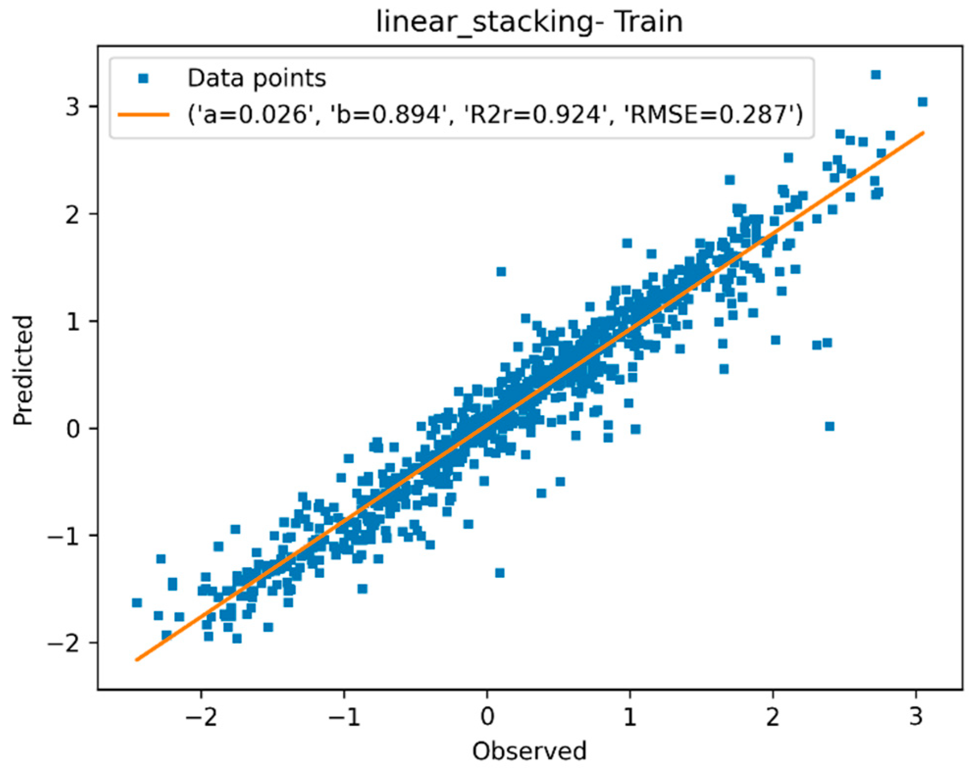
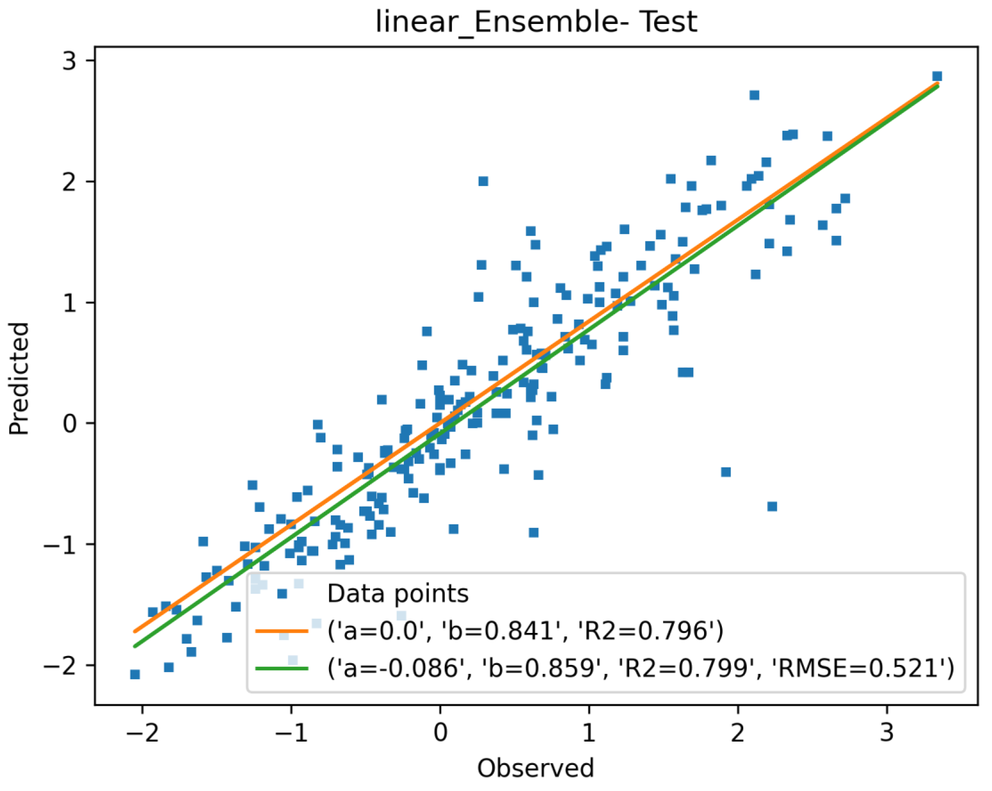
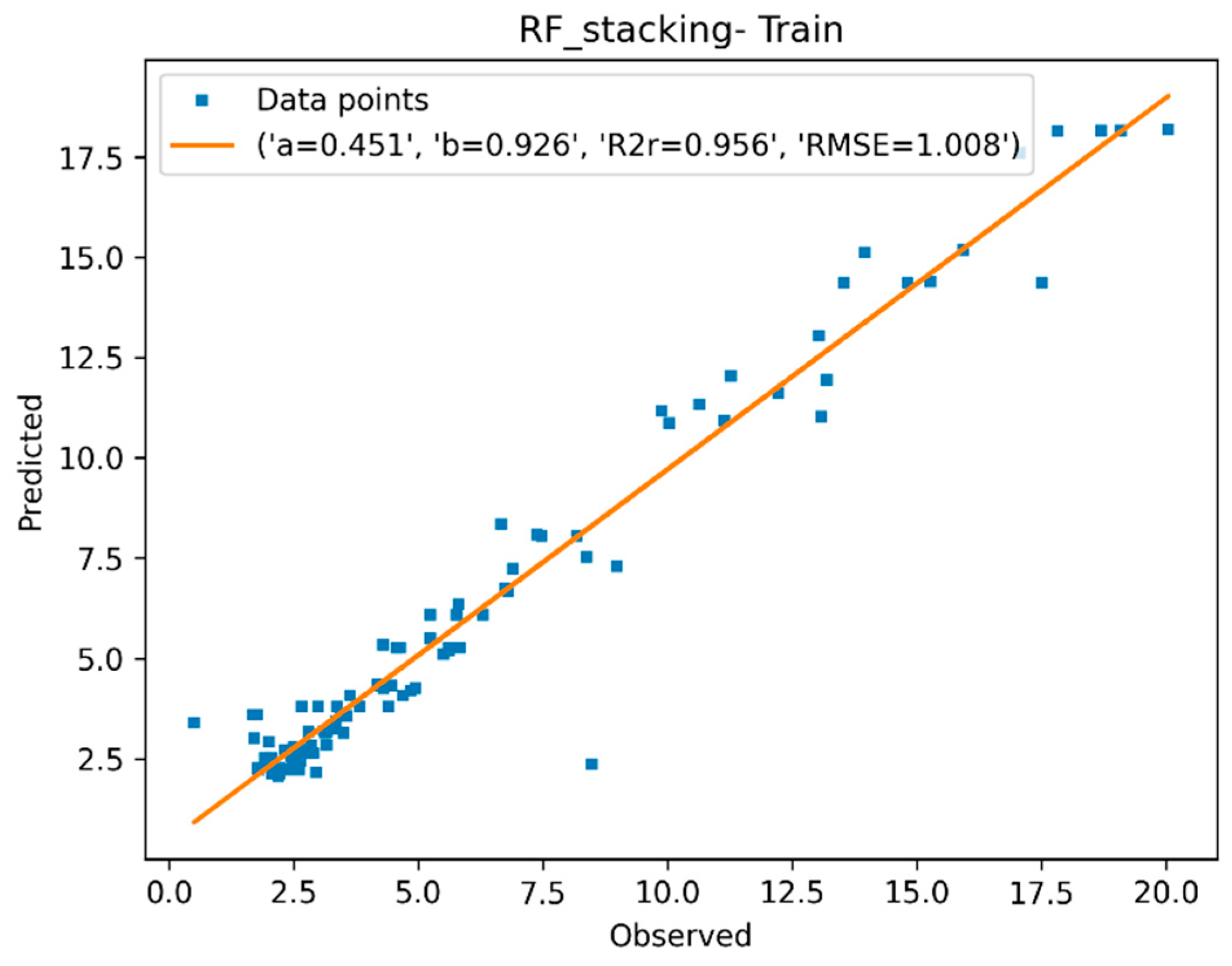
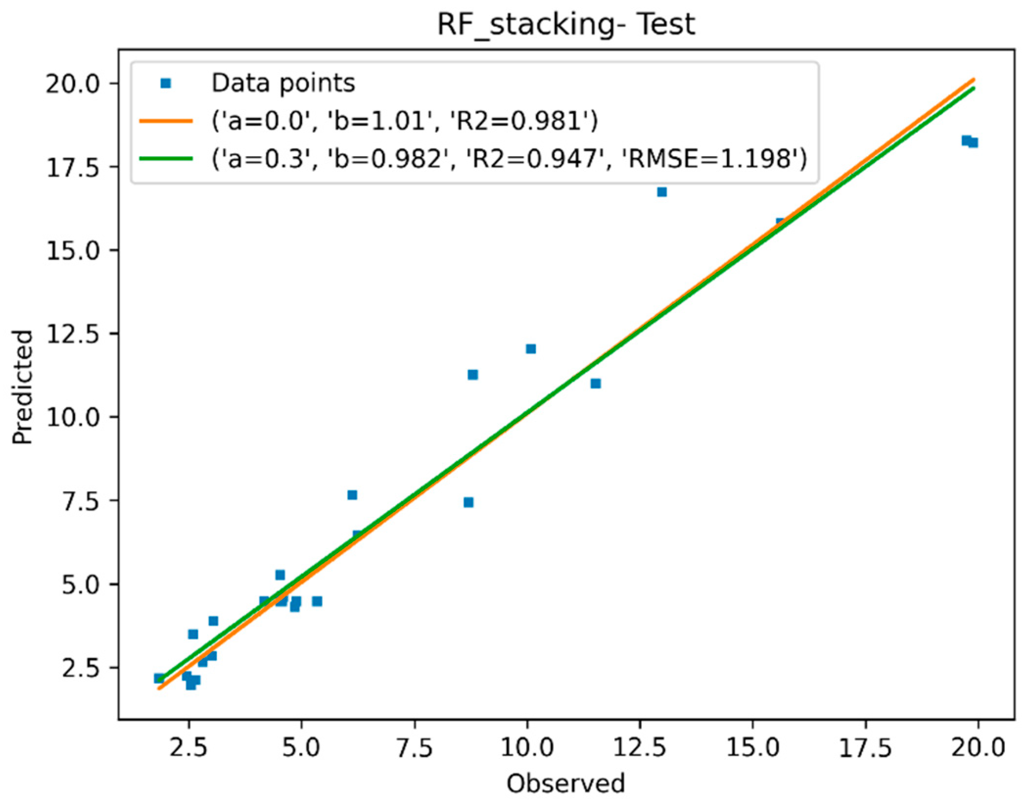
3.1.4. Descriptor Selection, Model Training, and Validation

A LASSO model was trained in order to identify highly correlated MFs to the biological activity. There were 233 molecular fragments selected in order to describe the chemical space on the training set.

The selected MFs were used to train the machine learning models that were built on Python while using the scikit-learn package. For each machine learning algorithm—support vector machine (SVM), gradient boosting machine (GBM), and random forest (RF)—a set of hyperparameters was optimized while using a repeated K-fold cross-validation grid. Individual models were elaborated using the optimized hyperparameters and a combination of these three models, as well the LASSO model, were evaluated in order to improve the predictive ability. Two ensemble techniques were explored; first, a linear combination of each model called “Linear ensemble”; and second, a stacking model utilizing an RF regressor. In

Table 1. Statistical parameters calculated for each model in the prediction of the biological activity (pIGC50) against T. pyriform using Least Absolute Shrinkage and Selection Operator (LASSO) as a feature selector for molecular fragments with different modeling strategies. In this case, the comparison uses Zhu’s work [39]. For further details see Supplementary files.

Software		R2-Train	MAE-Train	MAE-Test	R2-Test
CHARMING	LASSO	0.880	0.267	0.385	0.783
	SVM	0.904	0.215	0.389	0.784
	GBM	0.989	0.134	0.462	0.706
	RF	0.963	0.150	0.431	0.723
	RF-Stck	0.897	0.224	0.398	0.769
	Linear-Ens.	0.924	0.191	0.360	0.799
	Multilinear	0.900	0.240	0.403	0.775
ZHU’s work	kNN-Dragon	0.92	0.22	0.27	0.85
	kNN-MolconnZ	0.91	0.23	0.30	0.84
	SVM-Dragon	0.93	0.21	0.31	0.81
	SVM-MolconnZ	0.89	0.25	0.30	0.83
	ISIDA-kNN	0.77	0.37	0.36	0.73
	ISIDA-SVM	0.95	0.15	0.32	0.76
	ISIDA-MLR	0.94	0.20	0.31	0.81
	CODESSA-MLR	0.72	0.42	0.44	0.71
	OLS	0.86	0.30	0.35	0.77
	PLS	0.88	0.28	0.34	0.81
	ASNN	0.83	0.31	0.28	0.87
	PLS-IND	0.76	0.39	0.39	0.74
	MLR-IND	0.77	0.39	0.40	0.75
	ANN-IND	0.77	0.39	0.39	0.76
	SVM-IND	0.79	0.31	0.35	0.79

, the observed parameters for model evaluation are shown, as well as a comparison with Zhu’s work [39]. The study that was published by Zhu and co-workers reported the same difficulty in the description of the test set. The training set and test set show differences in the performance when the statistical parameters are analyzed. It reflects the inhomogeneity of the dataset. Nevertheless, the Charming performance was similar to the ones that also exclusively use molecular fragments and better to some of the approaches that use a summoning of different features. Some of the elaborated models in Zhu’s work also have moderate transferability to the test set, as it can be seen for the entries kNN-Dragon, kNN-MolconnZ, SVM-dragon, ISIDA-SVM, ISIDA-MLR, and OLS [39].

Although the gradient boosting machine (GBM) showed better fittings for the training set, the linear ensemble proved to have better performance for the test set. The linear ensemble shows higher R² and lower MAE values for the test set when compared to any of the machine learning models alone (respectively, 0.799 and 0.36 in Table 1; Figure 4 and Figure 5). The stacking using a random forest regressor has a similar performance to the other models. The R²-test is a measurement of the dispersion of the results along the linear regression; the $R_0^2$ and the K value measures how good the results are and if they can be used to predict new molecules [35,36,37]. Some compounds in the test set showed a large deviation from the model. A plausible reason for such a kind of poor fitting in the QSAR model is that such compounds may be acting in a different mechanism of action, having a different target biomolecule, despite showing the same biological result or having different binding modes due to conformational flexibility.

The correlation between each selected molecular fragment and biological activity can be retrieved from the LASSO model. The main MFs and their contributions are shown in Figure 6. The blue MFs have positive values and decrease toxicity. On the other hand, the red-colored fragments, such as the pattern 1-hydroxy-4-methoxy-benzene (upper right in Figure 6), increase the compound toxicity. That particular result could be associated with the similarity of this MF to the ubiquinol pattern. Therefore, compounds that have this moiety is supposed to interfere with vital processes to the cell, showing toxic activity.

3.2. Example 2

3.2.1. Data Set

The logarithm values of equilibrium constants for the extraction of Eu³⁺ for 128 compounds were retrieved from the literature [40,41]. The experimental procedures were performed at 25 °C and 0.1 mol/L. The compounds at the SDF file describe crown ethers complexing agents with different ring sizes and substitution patterns.

3.2.2. Standardization and Outlier Analysis

The standardization filter that was applied to the SDF file did not remove any molecule. The threshold value for each halogen atom was set at 6, the minimum molecular mass was 20, and the maximum 900. The outlier analysis removed 1 compound and the final work set has 127 molecules. The endpoints considered to be outliers were those that are higher than three σ away from the mean value (Figure 7).

3.2.3. Molecular Fragment Generation, Counting, and Preprocessing

There were generated 2787 MFs with three up to eight atoms. After the filtering step, the descriptors set has 189 MFs and all of the selected descriptors ranged between 0 and 1. The correlation threshold was used at 0.95.

3.2.4. Descriptor Selection Model Training and Validation

A LASSO model was trained in order to identify correlated MFs and the affinity constant logarithms (LogK). There were 22 molecular fragments selected to describe the chemical space of the training set.

The selected MFs were used to train the machine learning models, and the hyperparameters were optimized while using a repeated K-fold cross-validated grid. The optimized hyperparameters were used to build the individual models, the stacking, and the ensemble model.

Table 2. The observed statistical parameters for each generated model in the prediction of the affinity constant logarithms (LogK) of Eu³⁺ complexation. See Supplementary files for further details.

	R2-Train	RMSE-Train	RMSE-Test	R2-Test	${\mathit{R}}_0^2$	K
LASSO	0.951	1.067	1.197	0.949	0.981	1.011
SVM	0.963	0.926	1.325	0.941	0.976	0.976
GBM	0.994	0.728	1.918	0.86	0.95	0.937
RF	0.985	0.592	1.214	0.945	0.98	0.967
RF-Stk	0.956	1.008	1.198	0.947	0.981	1.010
Linear-Ens.	0.967	0.861	1.368	0.936	0.975	0.992
Multilinear	0.964	0.894	1.378	0.939	0.975	1.001

shows the observed parameters for model evaluation.

All of the training models have similar validation parameters. Special attention must be applied to the LASSO, and RF stacking that have the lowest RMSE values for the test set. Among them, the SVM has the lowest RMSE; in this case, it would be prudent to select this model in order to make predictions regarding this chemical space.

Figure 8 and Figure 9 show the training and the test plots for the RF-stacking model of the selected features, which has 0.997 for $R_0^2$. Interestingly, the highly polar molecule 3-amino-5-sulfosalicylic acid behaves as an outlier, at coordinates (8.49, 2.37). This behavior is probably due a different mode of coordination with ion Eu³⁺. This compound has four different functional groups and it behaves as a dipolar ion in solution.

The LASSO model has identified the main molecular fragments that are responsible for Eu³⁺ complexation. Figure 10 shows the main MFs and their contributions to the training model. The blue MFs have positive values and they increase the equilibrium constant. Conversely, the red MFs have negative values and they decrease the equilibrium constant. Rationalizing the chemical information that is brought with the fragments, we can say that compounds with amino or hydroxyl groups will have a greater affinity for Eu³⁺ complexation than ethers and amides groups. We can justify this pattern due to the charge relief in the coordination site by hydrogen bonding. That pattern acts as a better σ electron-donating group, stabilizing the cation more efficiently.

3.3. Example 3

3.3.1. Data Set

The biological anti-HIV activity for three different families of compounds—cyclic ureas (CU), 1-(2-hydroxyethoxy)methyl)-6-(phenylthio)thymines (HEPT), and tetrahydroimidazobenzo-diazepinones (TIBO)—were selected for building a QSAR model of their biological activity while using the Charming QSAR & QSPR. The CU, HEPT, and TIBO datasets have. respectively, 93, 84, and 73 compounds [42].

3.3.2. Standardization and Outlier Analysis

The standardization step on the SDF file did not remove any molecules. The threshold for each halogen atom was set at 6, the minimum molecular mass at 20, and the maximum at 900. The outlier analysis did not remove any compound for any dataset, and the final work set has all the molecules. The endpoints that were considered to be outliers were those that are higher than three σ away from the mean value.

3.3.3. Molecular Fragment Generation, Counting, and Preprocessing

For the CU, HEPT, and TIBO datasets, there were respectively, 5082, 7621, and 10,495 MFs generated containing from three up to 10 atoms. After the filtering step, the CU, HEPT, and TIBO have, respectively, 191, 128, and 226 MFs.

3.3.4. Descriptor Selection, Model Training, and Validation

A LASSO model was trained in order to identify the best set of MFs to describe biological activity. There were 47 molecular fragments selected for the CU derivatives set, 31 for the HEPT, and 18 for TIBO set in order to describe the chemical space of the training set.

The selected MFs were used in order to train the machine learning models, and the hyperparameters were optimized while using a repeated K-fold cross-validated grid. The optimized hyperparameters were used to build the individual models, the stacking, and the ensemble model.

Table 3. The values of observed statistical parameters for each model generated for the prediction of anti-HIV activity. See Supplementary files for further details.

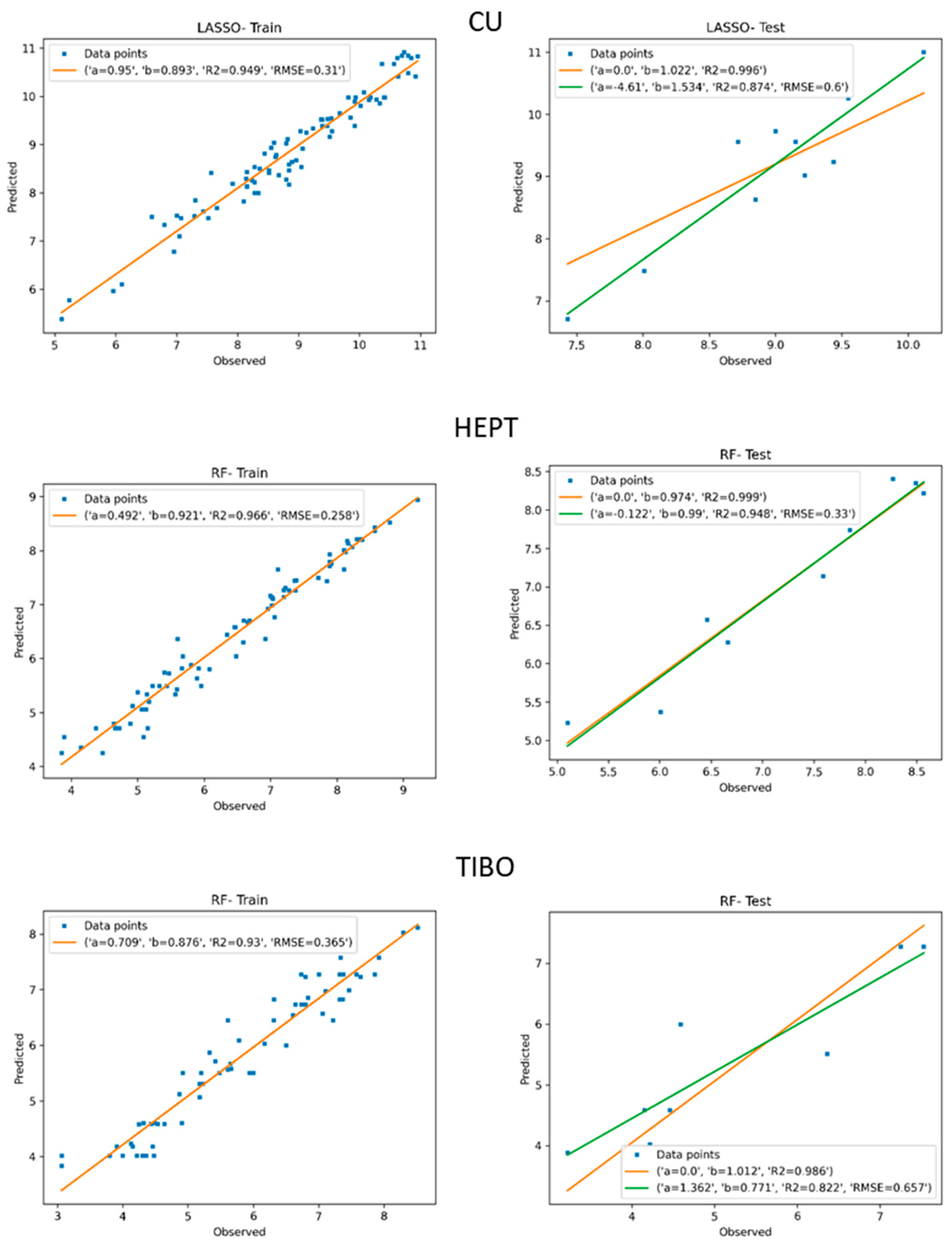
Set	Model	RMSE-Train	R2-Train	RMSE-Test	R2-Test	${\mathit{R}}_0^2$	K
CU	LASSO	0.310	0.949	0.600	0.874	0.996	1.022
	SVM	0.335	0.941	0.442	0.843	0.998	1.009
	GBM	0.210	0.993	0.949	0.483	0.993	0.928
	RF	0.277	0.963	0.629	0.661	0.996	0.968
	RF-Stk.	0.460	0.884	0.594	0.878	0.996	0.972
	Linear-Ens.	0.402	0.912	0.419	0.796	0.998	0.995
	Multilinear	0.244	0.966	0.863	0.832	0.992	1.031
HEPT	LASSO	0.292	0.954	0.918	0.837	0.990	1.065
	SVM	0.303	0.951	0.847	0.798	0.991	1.053
	GBM	0.275	0.976	0.434	0.889	0.997	0.972
	RF	0.258	0.966	0.330	0.948	0.999	0.974
	RF-Stk.	0.311	0.948	0.337	0.945	0.998	1.018
	Linear-Ens.	0.291	0.954	0.937	0.792	0.989	1.062
	Multilinear	0.265	0.962	1.071	0.844	0.987	1.078
TIBO	LASSO	0.529	0.858	0.868	0.687	0.976	1.018
	SVM	0.474	0.88	0.869	0.681	0.976	1.012
	GBM	0.348	0.951	0.721	0.797	0.983	1.011
	RF	0.365	0.930	0.657	0.822	0.986	1.012
	RF-Stk	0.564	0.832	1.114	0.506	0.962	1.023
	Linear-Ens.	0.493	0.873	0.874	0.681	0.975	1.009
	Multilinear	0.405	0.910	0.969	0.641	0.969	0.992

shows the observed parameters for each model evaluation. For the cyclic urea derivatives, the LASSO model has shown the best parameters for the test set (R² = 0.874, RMSE = 0.600), and a satisfactory description of the training set. For the HEPT compounds set, the Random Forest (RF) shows the best parameters for the training and test set ($R_{train}^2$ = 0.966, RMSE_train = 0.258, $R_{test}^2$ = 0.948, and RMSE_test = 0.330). For the TIBO group, the RF also shows the best parameters for the test set (R² = 0.822, RMSE = 0.657) and s satisfactory performance for the training set (Figure 11).

In Solov’ev and Varnek’s work, they create some models for describing the same dataset of compounds [43]. The best model for each of the three datasets is summarized below

Table 4. Statistical parameters calculated for each model in the prediction of anti-HIV activity for three different groups of molecules: cyclic ureas (CU), TIBO, and HEPT derivatives. ISIDA results were executed by Vernek’s group [43]. For further details see Supplementary files.

	Set	N-Train	R2-Train	N-Test	R2-Test
CHARMING	TIBO	65	0.93	8	0.822
	HEPT	75	0.966	9	0.948
	CU	83	0.949	10	0.874
ISIDA	TIBO	66	0.885	7	0.943
	HEPT	76	0.941	8	0.887
	CU	84	0.885	9	0.845

:

The ISIDA software was used in Solov’ev and Varnek’s works in order to describe the anti-HIV activity for the three referred datasets [43]. The CHARMING analysis clearly showed better results for the CU and HEPT datasets. Although CHARMING gave better fitting for the training set in the TIBO group, the best parameters for the test set were achieved while using ISIDA.

By retrieving the coefficients of each fragment assigned by LASSO model, the main structural patterns responsible for the anti-HIV activity were identified. Figure 12 shows an overview of the main MFs and their coefficients assigned by model elaboration for each dataset. The blue MFs have positive values; therefore, they contribute to increasing the log (1/IC₅₀)) endpoint (smaller IC₅₀ values). On the other hand, the red-colored MFs have negative values and decreases the log (1/IC₅₀)) (greater IC₅₀ values). Interpreting the chemical information that is embedded with the fragments, we can envisage the cyclic urea derivatives that have the pattern 3-(aminomethyl)aniline show smaller values of IC50 than the CUs that have 1-hydroxy-3-methoxy-5methyl arenes pattern. The HEPT compounds that show the 1,3-dimethylbenzene pattern have smaller values of IC50 than the HEPT compounds that have the N-(2-hydroxymethoxy)methyl pattern. Finally, the TIBO compounds that have the N-(2-bromobenzyl)ethanamine pattern show smaller values than the TIBOs, which have 1H-imidazo (4,5-c)pyridin-2(3H)-one pattern.

4. Final Considerations

Cheminformatic tools with predictive and qualitative models have proved to be valuable instruments in the development of biologically active compounds helping the optimization of the compound potency, selectivity, and physical-chemical properties. In this context, the Charming QSAR & QSPR provides an accessible alternative to developing statistical models for QSAR and QSPR. The use of Molecular Fragments (MFs) to describe the chemical space and their relation to the physical, chemical, and biological property has been developed and exemplified while using graph theory along with the SMILES notation. The application of MFs has the advantage of direct interpretability of the chemical information that is coded in form of molecular patterns. The Charming QSAR & QSPR was successfully applied to the prediction of pIGC50 of T. pyriform, the logK for complexation of ions Eu³⁺, and the log (1/IC₅₀) for three sets of compounds with anti-HIV activity.

References

- Varnek, A. Tutorials in Chemoinformatics, 1st ed.; Wiley: Hoboken, NJ, USA, 2017; pp. 3–278. [Google Scholar]
- Lounkine, E.; Batista, J.; Bajorath, J. Random molecular fragment methods in computational medicinal chemistry. Curr. Med. Chem. 2008, 15, 2108–2121. [Google Scholar] [CrossRef] [PubMed]
- Ruggiu, F.; Gilles, M.; Varnek, A.; Horvath, D. ISIDA Property-Labelled Fragment Descriptors. Mol. Inform. 2010, 29, 855–868. [Google Scholar] [CrossRef] [PubMed]
- Varnek, A.; Fourches, D.; Hoonakker, F.; Solov’ev, V.P. Substructural fragments: An universal language to encode reactions, molecular and supramolecular structures. J. Comput. Aid. Mol. Des. 2005, 19, 693. [Google Scholar] [CrossRef] [PubMed]
- Baskin, I.I.; Varnek, A. Building a chemical space based on fragment descriptors. Comb. Chem. High Throughput Screen. 2008, 11, 661–668. [Google Scholar] [CrossRef] [PubMed]
- Salum, L.B.; ·Andricopulo, A.D. Fragment-based QSAR: Perspectives in drug design. Mol. Divers. 2009, 13, 277. [Google Scholar] [CrossRef] [PubMed] [Green Version]
- Gaspar, H.A.; Baskin, I.I.; Gilles, M.; Horváth, D.; Varnek, A. GTM-Based QSAR Models and Their Applicability Domains. Mol. Inform. 2015, 34, 348–356. [Google Scholar] [CrossRef]
- Solov’Ev, V.P.; Varnek, A.; Wipff, G. Modeling of Ion Complexation and Extraction Using Substructural Molecular Fragments. J. Chem. Inf. Comput. Sci. 2000, 40, 847–858. [Google Scholar] [CrossRef]
- Varnek, A.; Fourches, A.P.D.; Horvath, D.; Klimchuk, O.; Gaudin, C.; Vayer, P.; Solov’Ev, V.P.; Hoonakker, F.; Tetko, I.; Gilles, M. ISIDA-Platform for Virtual Screening Based on Fragment and Pharmacophoric Descriptors. Curr. Comput. Drug Des. 2008, 4, 191–198. [Google Scholar] [CrossRef]
- Pirzada, S. Applications of graph theory. PAMM 2007, 7, 2070013. [Google Scholar] [CrossRef]
- Khursan, S.L.; Ismagilova, A.S.; Spivak, S.I. A graph theory method for determining the basis of ho-modesmic reactions for acyclic chemical compounds. Dokl. Phys. Chem. 2017, 474, 99. [Google Scholar] [CrossRef]
- Balaban, A.T. Applications of graph theory in chemistry. J. Chem. Inf. Model. 1985, 25, 334–343. [Google Scholar] [CrossRef]
- Manimekalai, S.; Mary, U.; Lavanya, M. Computation of topological Indices using python program for chemical graph structure. J. Phys. Conf. Ser. 2018, 1139, 012060. [Google Scholar] [CrossRef]
- Takata, M.; Lin, B.-L.; Xue, M.; Zushi, Y.; Terada, A.; Hosomi, M. Predicting the acute ecotoxicity of chemical substances by machine learning using graph theory. Chemosphere 2019, 238, 124604. [Google Scholar] [CrossRef] [PubMed]
- Ivanciuc, O. QSAR comparative study of Wiener descriptors for weighted molecular graphs. J. Chem. Inf. Comput. Sci. 2000, 40, 1412–1422. [Google Scholar] [CrossRef]
- Hayat, S.; Wang, S.; Liu, J.-B. Valency-based topological descriptors of chemical networks and their applications. Appl. Math. Model. 2018, 60, 164–178. [Google Scholar] [CrossRef]
- Randić, M.; Novič, M.; Plavšić, D. Solved and Unsolved Problems of Structural Chemistry, 1st ed.; CRC Press: Boca Raton, FL, USA, 2016; pp. 23–198. [Google Scholar]
- Randić, M. On history of the Randić index and emerging hostility toward chemical graph theory. Match Commun. Math. Comput. Chem. 2008, 59, 5. [Google Scholar]
- Balaban, A.T. Chemical Graphs: Looking Back and Glimpsing Ahead. J. Chem. Inf. Model. 1995, 35, 339–350. [Google Scholar] [CrossRef]
- Vinogradova, M.G.; Fedina, Y.A.; Papulov, Y.G. Graph theory in structure–property correlations. Russ. J. Phys. Chem. A 2016, 90, 411–416. [Google Scholar] [CrossRef]
- Dobrowolski, J.C. The structural formula version of graph theory. Match Commun. Math. Comput. Chem. 2019, 81, 527. [Google Scholar]
- Domenech, R.G.; Gálvez, J.; Ortiz, J.V.J.; Pogliani, L. Some new trends in chemical graph theory. Chem. Rev. 2008, 108, 1127. [Google Scholar] [CrossRef]
- Weininger, D. SMILES, a chemical language and information system. 1. Introduction to methodology and encoding rules. J. Chem. Inf. Model. 1988, 28, 31–36. [Google Scholar] [CrossRef]
- Weininger, D.; Weininger, A.; Weininger, J.L. SMILES. 2. Algorithm for generation of unique SMILES notation. J. Chem. Inf. Model. 1989, 29, 97–101. [Google Scholar] [CrossRef]
- RDKit. Open Source Toolkit for Cheminformatics. Available online: http://www.rdkit.org (accessed on 30 October 2020).
- Pedregosa, F.; Varoquaux, G.; Gramfort, A.; Michel, V.; Thirion, B.; Grisel, O.; Blondel, M.; Pret-tenhofer, P.; Weiss, R.; Dubourg, V.; et al. Scikit-learn: Machine learning in python. J. Mach. Learn. Res. 2011, 12, 2825. [Google Scholar]
- Verma, R.P.; Hansch, C. An approach toward the problem of outliers in QSAR. Bioorganic Med. Chem. 2005, 13, 4597–4621. [Google Scholar] [CrossRef]
- Kim, K.H. Outliers in SAR and QSAR: Is unusual binding mode a possible source of outliers? J. Comput. Mol. Des. 2007, 21, 63–86. [Google Scholar] [CrossRef]
- Toropov, A.A.; Toropova, A.P.; Rasulev, B.F.; Benfenati, E.; Gini, G.; Leszczynska, D.; Leszczynski, J. Coral: QSPR modeling of rate constants of reactions between organic aromatic pollutants and hy-droxyl radical. J. Comput. Chem. 2012, 33, 1902–1906. [Google Scholar] [CrossRef]
- Toropova, A.P.; Toropov, A.A.; Rasulev, B.F.; Benfenati, E.; Gini, G.; Leszczynska, D.; Leszczynski, J. QSAR models for ACE-inhibitor activity of tri-peptides based on representation of the molecular struc-ture by graph of atomic orbitals and smiles. Struct. Chem. 2012, 23, 1873–1878. [Google Scholar] [CrossRef]
- Benfenati, E.; Toropov, A.; Toropova, A.P.; Manganaro, A.; Diaza, R.G. coral Software: QSAR for Anticancer Agents. Chem. Biol. Drug Des. 2011, 77, 471–476. [Google Scholar] [CrossRef]
- Sklearn.linear_model.Lasso—Scikit-Learn 0.23.2 Documentation. Available online: https://scikit-learn.org/stable/modules/generated/sklearn.linear_model.Lasso.html (accessed on 30 October 2020).
- Feature Selection—Scikit-Learn 0.23.2 Documentation. Available online: https://scikit-learn.org/stable/modules/feature_selection.html#l1-feature-selection (accessed on 30 October 2020).
- Feature Selection Using SelectFromModel and LassoCV—Scikit-Learn 0.23.2 Documentation. Available online: https://scikit-learn.org/stable/auto_examples/feature_selection/plot_select_from_model_diabetes.html#sphx-glr-auto-examples-feature-selection-plot-select-from-model-diabetes-py (accessed on 30 October 2020).
- Alexander, D.L.J.; Tropsha, A.; Winkler, D.A. Beware of R2: Simple, Unambiguous Assessment of the Prediction Accuracy of QSAR and QSPR Models. J. Chem. Inf. Model. 2015, 55, 1316–1322. [Google Scholar] [CrossRef] [Green Version]
- Tropsha, A. Best Practices for QSAR Model Development, Validation, and Exploitation. Mol. Inform. 2010, 29, 476–488. [Google Scholar] [CrossRef]
- Gramatica, P.; Sangion, A. A historical excursus on the statistical validation parameters for QSAR models: A clarification concerning metrics and terminology. J. Chem. Inf. Model. 2016, 56, 1127. [Google Scholar] [CrossRef]
- Schultz, T.W.; Netzeva, T.I. Development and evaluation of QSARs for ecotoxic endpoints: The ben-zene response-surface model for Tetrahymena toxicity. In Modeling Environmental Fate and Toxicity; Cronin, M.T.D., Livingstone, D.J., Eds.; CRC Press: Boca Raton, FL, USA, 2004; Volume 4, Chapter 12; pp. 265–284. [Google Scholar]
- Zhu, H.; Tropsha, A.; Fourches, D.; Varnek, A.; Papa, E.; Gramatica, P.; Oberg, T.; Dao, P.; Cherkasov, A.; Tetko, I.V. Combinatorial QSAR Modeling of Chemical Toxicants Tested against Tetrahymena pyriformis. J. Chem. Inf. Model. 2008, 48, 766. [Google Scholar] [CrossRef] [Green Version]
- The IUPAC Stability Constants Database, SC-Database (No Longer Available Commercially) and Mini-SCDatabase. Available online: http://www.acadsoft.co.uk/scdbase/scdbase.htm (accessed on 30 October 2020).
- Solov’ev, V.P.; Tsivadze, A.Y.; Varnek, A. A New approach for accurate QSPR modeling of metal complexation: Application to stability constants of complexes of lanthanide ions Ln3+, Ag+, Zn2+, Cd2+, and Hg2+ with organic ligands in water. Macroheterocycles 2012, 5, 404. [Google Scholar] [CrossRef] [Green Version]
- Horvath, D.; Bonachera, F.; Solov’Ev, V.P.; Gaudin, C.; Varnek, A. Stochastic versus Stepwise Strategies for Quantitative Structure−Activity Relationship GenerationHow Much Effort May the Mining for Successful QSAR Models Take? J. Chem. Inf. Model. 2007, 47, 927–939. [Google Scholar] [CrossRef]
- Solov’ev, V.P.; Varnek, A. Anti-HIV activity of HEPT, TIBO, and cyclic urea derivatives: Structure-property studies, focused combinatorial library Generation, and hits selection using substructural mo-lecular fragments method. J. Chem. Inf. Comput. Sci. 2003, 43, 1703–1719. [Google Scholar]