1. Introduction
In this paper, we consider the problem of a single party, called the principal, creating contracts to delegate a task to a group of different agents. Incentive contracts stimulate the agents to act in the principal’s interest by compensating them for achieving two goals: (i) they accept the offered contract (i.e., the contract is subject to the individual rational (IR) constraint); and (ii) they exert the effort at a desired level determined by the compensation spelled out in the contract (i.e., the contract is subject to the incentive compatible (IC) constraint). Such incentive contracts have been used for many practical problems ranging from corporate finance to strategic behavior in politics to institutional design [
1,
2,
3,
4,
5,
6,
7,
8,
9,
10].
In a dynamic setting, the goal as before is to incentivize agents to exert the desired effort over the planning horizon. To achieve this, each contract defines a stream of payoff amounts, which depend on the effort exerted by the corresponding agent. In the framework we consider in this paper, the agent’s effort process is not perfectly observable, possibly due to the cost or the difficulty of monitoring it. Instead, the principal observes a noisy output process, which is a result of the effort exerted by the agent. This proxy results in information asymmetry about the agent’s effort (the agent knows it, but the principal can only infer it from a proxy). The asymmetric information can create a potential moral hazard problem in the contract design [
11]. The system efficiency is degraded as the first-best contract is not admissible. Given all these considerations, the incentive contract must solve the moral hazard problem and maximize the principal’s utility.
This fundamental incentive contract problem in the case of a single agent has been explored in many settings [
7,
12,
13,
14,
15]. We consider the problem as a special case of stochastic Stackelberg differential games played between a principal and an agent. The principal expects the agent to exert a targeted level of effort and knows ex ante that once the agent has accepted the contract, it has no incentive to deviate from this target level (thus bypassing any resulting moral hazard). This incentive-compatible condition can be satisfied if the agents’ actions form a subgame perfect Nash equilibrium. However, finding such a globally optimal contract over the planning horizon is not trivial. The dynamic moral hazard problem has been studied in a discrete-time setting, where the state space explodes exponentially in the size of the planning horizon (the curse of dimensionality in dynamic programming) [
16]. Holmstrom and Milgrom [
17] proposed a continuous-time model. In this setting, the agent’s output process is represented by a stochastic differential equation (SDE) whose drift term is controlled by the agent’s effort. As a result, the continuous-time incentive contract problem is a limit of discrete-time dynamic games whose number of stages becomes unbounded in any finite interval. Some extensions of their work include Schattler and Sung [
18], Sung [
19], and Muller [
20]. In recent years, following the groundbreaking work of Sannikov [
21], there has been a resurgence of interest in the dynamic contract theory. The main contribution of [
21] was to parameterize the incentive-compatible constraint at each epoch using the Martingale representation theorem. As a consequence, we can decouple the principal’s and the agent’s problems by representing the agent’s effort as a function of a parameter. The principal’s problem can then be solved by dynamic programming (more specifically, a Hamiltonian Jacobi–Bellman equation) for the incentive contract [
3,
15,
21,
22].
A significant extension of the single-agent incentive contract is multiagent incentive contracts. For example, a company hires multiple employees to collaborate on a project. Since employees with correlated responses may have different capabilities and utility functions, designing contracts separately for each is not viable. Koo et al. [
23] presented the first extension of multiagent incentive contracts that initiated a stream of literature for team incentives using the Martingale approach [
24,
25,
26,
27]. In the multiagent setting, new challenges arise due to varied interactions between agents. For example, an arbitrary agent may compare both its effort and payoff with others; such a phenomenon is called inequity aversion [
28]. Goukasian and Wan showed that inequity aversion is present in multiagent incentive contracts [
29], and agents’ comparisons lower their exerted effort levels.
The critical condition for the existence of effective multiagent incentive contracts is that agents’ actions at each epoch must form a Nash equilibrium. This equilibrium then incentivizes each agent to choose the principal’s desired actions and nullifies the moral hazard in the contract. The conditions for the existence of this equilibrium is still an open question. Prior work [
27] assumed that the existence conditions are satisfied in their setting without verification. The agents’ optimal actions constituting a Nash equilibrium led to a circular argument. Yet, characterizing the existence of a Nash equilibrium in multiagent contracts is non-trivial [
30,
31,
32], more so in the dynamic setting considered in this work. The following example demonstrates the importance of investigating the existing conditions in a static matrix game setting. A principal chooses to compensate
to two agents as either low (
L) or high (
H) payoff, i.e.,
for
. Agents putting effort into a project generate output denoted as
at levels
A or
B.
The principal desires to stimulate Agent 1 to exert output
A and Agent 2 to exert output
B. The outcomes of signing contracts are represented by the matrices in
Table 1, where each entry is the principal’s and agent’s utility received from the contract. If these two contracts are signed separately, the unique equilibria are
with Agent 1 and
with Agent 2.
We now assume that two agents’ outputs are aggregated in a linearly additive way. In this case, the principal’s dominant policy is . Notice that the existence and the number of equilibria may vary with the agents’ utility functions . Three possible outcomes for the contracts are below:
Unique Nash equilibrium: Assume that the utility of each agent is only dependent on its payoff, i.e.,
. The agents’ best responses are
. With a fixed
, their utility follows
Table 2.
Multiple Nash equilibria: Assuming that the principal rewards whoever delivers
B an additional unit of compensation, there exists two Nash equilibria,
and
, for which their utility follows
Table 3.
No Nash equilibrium: Assuming that the utility of each agent is affected by the other’s action such that the principal would reward the agents when their outputs match, i.e.,
if
, then there is no Nash equilibrium, as seen in
Table 4.
Our goal in this paper is to find conditions that guarantee the existence of a unique multiagent Nash equilibrium in incentive contracts. We see that even if the existence problem is settled [
27], the uniqueness of the multiagent Nash equilibrium must still be tackled. Characterizing unique equilibrium has practical value as coordinating agents to select the optimal Nash equilibrium is improbable; it also has theoretical value as the optimal contracts with a set of equilibria is computationally intractable. Using a fixed-point theorem (specifically, the Kakutani fixed-point theorem), we prove the existence of a subgame perfect Nash equilibrium. The existence conditions include the assumption that all agents are risk-averse and the interactions of all agents’ actions on other’s output follow a concave function. With a slight strengthening of the condition on the Hessian matrix of the interaction functions and with the use of the theorem of Gale and Nikaido [
33] and Kojima and Saigal [
34], we prove that the equilibrium is unique. These results then enable us to develop a provably convergent iterative procedure to solve for the incentive contracts.
Unlike the infinite horizon setting of [
21], we consider the problem with a finite horizon where the terminal condition may be path-dependent. Such terminal conditions are widely used in modeling options, mortgage defaults, and car leasing, thus enhancing the applicability of the methodology.
The general notation used in the rest of this paper is as follows. A set of indices . Bold variables are vectors or matrices of random variables or functions. In equilibrium analysis for the agent, we denote a vector as , where indicates the variable associated with the agent. indicates that the variable is associated with the principal. is a variable that deviates from x in the domain of x. is the Jacobian, and is the Hessian of the function F of x.
The remainder of this paper is organized as follows. In
Section 2, we describe the setting of multiagent incentive contracts. In
Section 3, we characterize the agents’ optimal responses and prove the existence of a unique Nash equilibrium. We then formulate the principal’s problem as a Hamilton–Jacobi–Bellman equation. We also give an iterative procedure to implement the optimal incentive contracts. In
Section 5, we draw the final conclusion.
3. Incentive-Compatible Constraints
In this section, we characterize an individual agent’s optimum action within given multiagent contracts.
3.1. Parametrization of the Individual Agent’s Problem
We analyze an arbitrary
agent’s optimum action given the other agents’ optimum actions. Without loss of generality, we reformulate the analysis of the prior work [
3,
21] under a new multiagent contracts setting.
In dynamic Stackelberg games, one commonly defines the continuation value
(the value function in dynamic programming) when the optimal actions
are taken by all agents in
, i.e., the agent
i’s conditional expected optimal discounted utility received from
t to
T, as follows,
where
is the filtration generated by the Brownian Motions
and
.
We now describe the dynamics of for a single agent with a path-dependent terminal condition as follows:
Proposition 1. There exists an adapted process such that the continuation value of the agent is represented by the process:Conversely, a process satisfying the SDE is the agent’s continuation value. Proof. Given fixed and optimal n-agents’ efforts
and the filtration
, we have:
is an
-Martingale, i.e., for any
, using (
6) and the iterated conditional expectation, it is readily seen that
. From the Martingale representation theorem [
3], we obtain the existence of adapted processes
and
such that:
From (
5), it is easily seen that (
6) can be rewritten as:
and using Ito’s lemma, we obtain the dynamics:
Equating the above two dynamics of gives the result. □
The expansion of the state space (when compared to [
21]) is needed to accommodate the path-dependent terminal condition, requiring the vector
to be a part of the state space. Dynamic contracts between the principal and the
agent must specify: (a) the instantaneous compensations
and (b) two processes
and
as the sensitivity of the agent’s continuation value
to the output
and terminal process
, respectively.
Given a contract
, we use the one-shot deviation principle to derive the necessary condition for the optimality of the effort
with given
. This optimality condition is equivalent to the IC constraint in (
4). Such an optimality condition holds for an arbitrary
agent’s
given
.
Proposition 2. For any fixed , the contracted compensation for the agent i is implementable if and only if satisfies:for all . Proof. Let
be the optimal effort vector, and let the effort of the
agent, for a fixed
, be:
We denote
. Choosing actions
will change the dynamics of
and
. To obtain the new dynamics, we apply Girsanov’s theorem with the kernel
. The new dynamics adapted to Brownian motions
and
on the space
are given by:
Substituting in (
1) and Proposition 1 under
, the dynamics of
become:
Since is optimal, the drift of this SDE must be non-positive. This completes the proof. □
These two propositions decouple the principal’s and an arbitrary agent’s problem. To specify the target efforts that are not observable, the principal can incentivize the agent by recommending a sensitivity level . With n agents, the Nash equilibrium is equivalent to finding the optimal jointly. The principal can create a contract with: (a) functions for for each agent i; and (b) functions of the sensitivity that specify the target effort processes. Hence, we create multiagent contracts that provide consistent information for all agents over the planning horizon, which are thus implementable.
Characterizing implementable multiagent contracts require that the actions of the agents form a multiagent Nash equilibrium at each epoch . We note that in our formulation, there are interactions among n-agents both in the instantaneous utility and drift term of output processes for all . The principal thus chooses a target effort level , which form a Nash equilibrium among agents, so that each agent is disincentivized to deviate from the target when the other agents do not, i.e., implementing the targeted .
3.2. Multiagent Nash Equilibrium
We now prove the existence of a Nash equilibrium among n-agents’ best responses (
7) at a fixed epoch
t. Bellman’s principle of optimality guarantees that it is sufficient to show the existence of a Nash equilibrium within the Hamiltonian of the IC constraint to prove the existence of a subgame perfect Nash equilibrium.
We need the following assumptions on the functions and for all :
is twice continuously differentiable, decreasing in , and concave in .
is twice continuously differentiable, increasing and concave in .
For each i and , and while as .
The set is nonempty and compact.
There exists an such that , and as , for all i and .
for each .
The single-agent contract in [
21] and the multiagent contracts in [
24] are special cases of the functions above with
u separable in
and
and
. Assumption 4 is satisfied because an arbitrary agent can choose effort
to have zero utility. Assumption 6 is valid because
if
. With these assumptions, we can show the following lemmas.
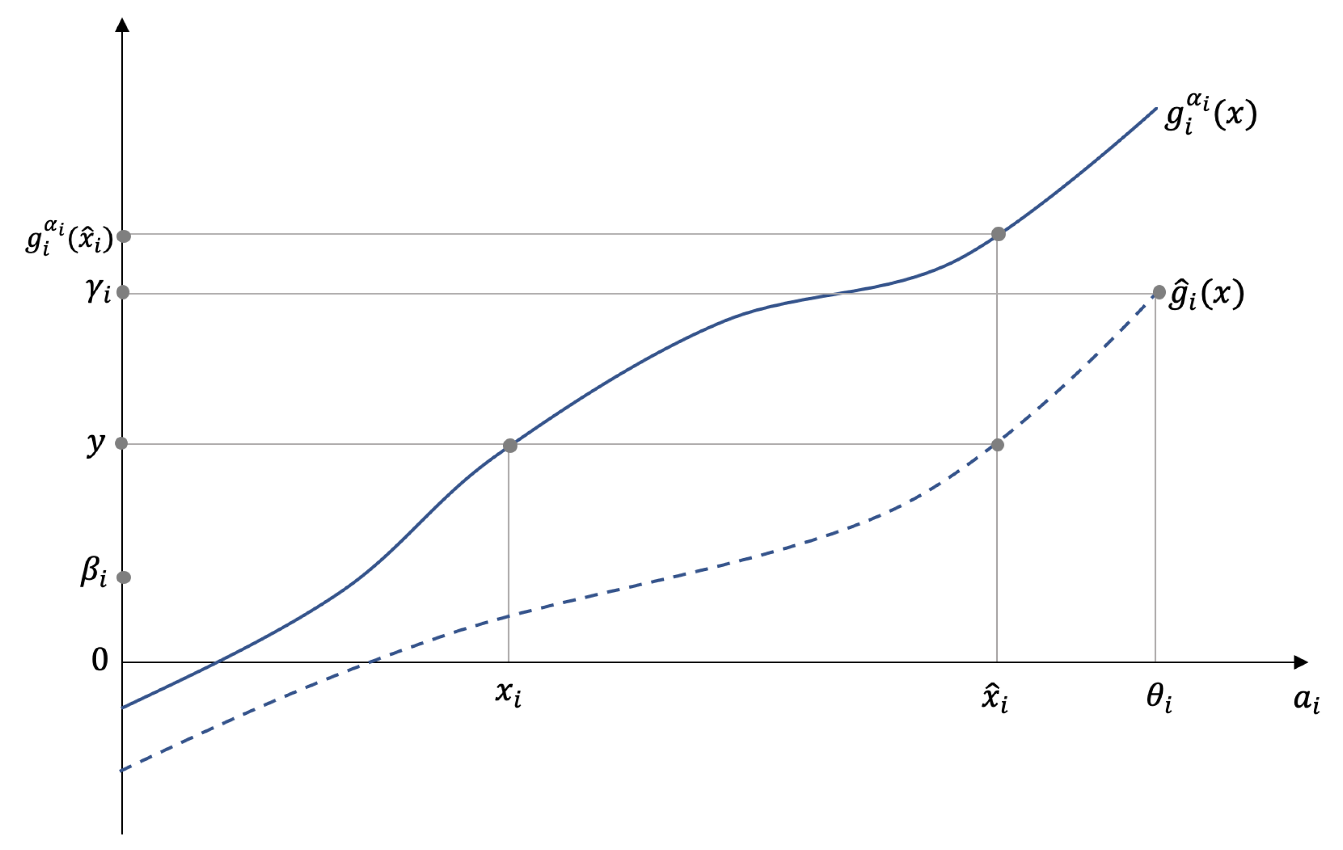
Lemma 1. Let , and we define: is continuously differentiable and monotonically increasing as a function of x in the domain . Furthermore, there exist such that for each and , has a solution.
Proof. is well defined from Assumption 3 on
, i.e., it is nonzero, and its monotonicity follows from the concavity of
and
. We define:
Let
be the
agent’s greatest effort, i.e.,
. Define
and
sufficiently large so that
is nonempty. This exists as
is an increasing function in
Figure 1.
For arbitrary , we define . Such an exists because the function is monotonically increasing. Now, for any , the function and . The result follows from the continuity of and the intermediate value theorem. □
Applying Lemma 1 to all agents , we define a set . We can now rigorously define the multiagent Nash equilibrium as follows.
Definition 1. The multiple agents’ effort is called a Nash equilibrium if and only if an arbitrary agent’s deviation from the stipulated effort level in while the other agents follow their stipulated actions will result in a loss to the agent, i.e., for each , Note that the multiagent equilibrium is independent of . We now prove a simple lemma to characterize the equilibrium:
Lemma 2. For all and each and , if satisfying (8) exists, it lies in the set . Proof. For any given contract
, let
be a Nash equilibrium for each
, and let
for some
and
. Thus,
. However, from Property 6,
Thus, is not a Nash equilibrium for , a contradiction. The result follows from the fact that as is continuous, thus it cannot be strictly negative on a set of measure zero in . □
The following corollary shows that agents continue to abide by the conditions of the contracts until the termination epoch.
Corollary 1. A consequence of the implementation of the Nash equilibrium is that no agent has an incentive to leave the contracts before the terminal epoch T.
Proof. As is seen in the proof of Lemma 2, when agents’ actions form a multiagent Nash equilibrium, each agent receives a positive utility in any finite interval, thus making each agent’s total utility an increasing function of its continuation value. Therefore, no agent is motivated to deviate from the target action before the termination epoch T. □
The theorem below establishes the existence of such an equilibrium in each given epoch t.
Theorem 1. For each given and , there exists a subgame perfect Nash equilibrium for every .
Proof. For a fixed agent
, given the concavity of the functions in Proposition 1, a necessary and sufficient condition for
to solve the optimization problem is that
. We note that as defined in (
8),
.
We now define a point-to-set map,
Note that
, where
is the set of all compact and convex subsets of
. To see that
is an upper hemicontinuous point to set map, let
be a sequence in
that converges to
. Furthermore, let
for each
k such that
converges to
. To see that
is in
, we note that
is such that
. From the definition of
in Lemma 1, it is a continuous function of
and
x, thus
for each
i. The existence of the Nash equilibrium now follows from Lemma 2, Property 4, in the assumptions, and the Kakutani fixed-point theorem [
36]. □
3.3. On the Uniqueness of the Nash Equilibrium in Multiagent Contracts
The individual incentive contract assumes that, if multiple subgame perfect Nash equilibria exist, the principal has the power to choose her or hiss preferred one. However, if multiple equilibria exist in the multiagent contracts, first all equilibria must be found, and then, we look for plausible selection criteria to convince the agents to implement a specific chosen equilibrium. To avoid this computational problem at each epoch t, we impose reasonable and mild additional conditions to guarantee a unique Nash equilibrium. We now state these conditions:
is strictly concave in and for each and each .
Let for each
,
for each
and, similarly,
. The matrix
(
) is such that its
ith row is strictly diagonally dominant (diagonally dominant) in variables
, i.e.,
Remark 1. Comments on the uniqueness conditions of the Nash equilibrium of agents:
- 1.
Condition 1 stipulates that the optimal effort the agents exert is unique and also has a negative effect on their instantaneous utility, i.e., the marginal utility as a function of the agent i’s effort is negative.
- 2.
Condition 2 states that agent i’s particular decision mostly affects the decrease in his or her marginal utility. In contrast, the other agents’ efforts have a minor effect (note the strict concavity implies that is negative).
- 3.
The signs of are related to whether is a strategic complement or a strategic substitute [36]. Diagonal dominance thus assumes that the magnitude of the effect of any agent’s actions exceeds the magnitude of the combined strategic effects of all the other agents’ actions.
We now prove a result:
Lemma 3. Let and satisfy Conditions 1 and 2 above and be as defined in Lemma 1, and . The Jacobian matrix of g, is then a P-matrix, i.e., has all principal minors positive.
Proof. We first show that
is a strictly row diagonally dominant Jacobian matrix. Note that, suppressing the argument
,
, we obtain:
The row dominance now follows from Condition 2 and the observation that
,
,
, and
in the domain
. Furthermore, it is easy to see that each principal submatrix of
is also strictly row diagonally dominant. Using Gershgorin’s theorem [
37], it follows that all the principal submatrices of
are nonsingular. We now let
B be any such principal submatrix and let
be the diagonal matrix of its diagonal elements and
the matrix of its off-diagonal elements. Define
for each
.
is strictly row diagonally dominant for each
t, and since
,
is also positive. Thus,
is a
P-matrix. □
Theorem 2. Assume Conditions 1 and 2 above hold. Then, for each epoch , the Nash equilibrium is unique.
Proof. From the strict concavity of
and (
8), we see that for given
and
,
is a Nash equilibrium if and only if:
Let
be the largest effort agent
i can put, as found in Lemma 1; define
, and consider the set
. Using the
P-matrix property of
, the fact that
is a hypercube and the Gale–Nikaido theorem [
33] (or [
34]), we see that
g maps
homeomorphically onto
. The uniqueness follows as
. □
4. The Optimal Multiagent Contracts
In this section, we solve the optimal multiagent contracts given that n-agents put effort at equilibrium in
Section 3. We denote the principal’ controls as
. Define:
With the parameterized IC constraints and a well-defined set of Nash equilibria
for given
for all
, the principal’s problem is as follows:
We note here that, in general, getting all Nash equilibrium points is generally not possible, but if it is unique, the problem (
10) can be solved. Let
be the present value of the conditional expectation of the continuation value of the principal at time
t when the policy
is followed in
. Thus:
and note that
is a random process. Therefore, define:
In case the optimal solution exists, then is a adapted Martingale and thus has a zero drift, and for other ’s, its drift is non-positive. We now make the following assumption about the principal’s continuation value:
Assumption 1. We assume that the value has the following functional form in variables t, the n-agents’ continuation vector , the observed output vector , and the termination value descriptor vector .
represents the differentiability class regarding the scalar or the vector. In what follows, for the ease of exposition, we will shorten to whenever there is no possibility of confusion.
Remark 2. The state space includes to assure that the vector process is Markov. In the special case that (i.e., an infinite time horizon with the transversality condition), the state space does not contain t, as in [3]. Then, the optimum utility received by the principal, following the optimal control
, can also be written as:
Note that, at epoch
t,
is realized, and
is determined by the control
. Following the argument of Proposition 1, we see that
, defined by (11) and (
13), is a
-adapted Martingale and thus has drift zero. Applying Ito’s multidimensional lemma and the dynamics of
,
, and
, we obtain the dynamics of
. Thus, we can solve for
F by setting the drift of its dynamics to zero.
To obtain the drift term, we recall the dynamics of the state variables. For notational convenience, we let
,
,
, and
. Let
be the Cholesky factor of
(i.e.,
), the covariance matrix of
. There exists a process
, a vector of
n independent Brownian motions, with:
Using Proposition 1, we get:
and similarly for the dynamics of
using (
2).
We define a differential operator
as a function of the control vector
as follows,
where
and
are the first and second derivative matrices of
with respect to
. We note here that in the above, we suppressed the superscript in
.
Applying the multidimensional Ito’s lemma to (
13), we get the drift of the dynamics of
as:
We now prove the theorem that verifies Assumption 1 and sets up a Hamilton–Jacobi–Bellman equation that solves the problem (
9):
Theorem 3. The principal’s problem can be formulated as the Hamilton–Jacobi–Bellman equation:Let its solution be and the control . and solve the optimization problem (9). Thus, Assumption 1 is verified. Proof. For the ease of notation, we define
and let
be the weak solution of the equation (
17) under control
.
Now, using an arbitrary control law
, such that
at the arbitrary time
t, with the state dynamics of
governed by the Brownian motions
and when
G solves the HJB equation, we see that:
for all
. Thus, we have, for each time
,
Integrating the above system from
t to
T, using Ito’s lemma to
, and integrating (which sets the stochastic integral to zero), we see that:
From the boundary condition, we also have
. Integrating the above expression and Inequality (
18), we obtain:
Since the control
was chosen arbitrarily,
as in (
12), the optimal solution to the problem (
9), we have:
To see the converse, let
and
solve the HJB
. Ito’s lemma gives, as in (
18) an Ito integral
J:
Using (
17) and the above with minor rearrangement and taking an expectation conditioned on
, we get:
Since
is a control and since
is the optimal continuation value under the optimal control
,
. Thus, combining with (
19), we get:
The theorem now follows since we have from the above inequalities for arbitrary t, and is the optimal contract. □
Iterative Algorithm for Solving Multiagent Contracts
Since adding an equilibrium constraint causes new computational issues, we propose here an iterative algorithm to obtain the optimal multiagent contracts in Theorem 3. The main idea is to integrate a numerical method for solving the HJB (i.e., Howard’s algorithm [
38]) with a fixed-point algorithm (i.e., Eaves–Saigal’s algorithm [
39]). For brevity, we denote the state variable at time
t by a time-generic vector
(note that the mesh width for each type of state may vary) and the control at time
t by
. We discretize the
plane by choosing uniform mesh widths
and a time step
such that
. We define the discrete mesh points
by:
Our goal is to compute an approximation
to the solution
in (
17) by discretization and a finite difference method.
Now, define the approximation for the Hamiltonian operator
in (
15) as
(we use a forward-in-time and central-in-space scheme) with the following approximations for gradients:
where
is a unit vector with one in the
entry and zero elsewhere. The
entry of the approximation for a Hessian (we only present the Hessian with respect to
) is:
We define the function and the principal’s value function under optimal control at time t as . We initialize with the boundary condition as the terminal conditions and the well-posed conditions for the state space. Especially, we note that, in an n-agents’ contract, when -agents have zero continuation values w, we need to first solve an -agents subproblem as a boundary condition. In the step in the policy iteration, policy evaluation under controls is conducted by solving the approximation of the PDE as .
Since the PDE under arbitrary control is well-posed, we can find a weak solution to
[
40]. We then (1) solve a fixed-point problem to find the agents’ unique optimal responses
and (2) use a greedy algorithm to improve the policy as:
Summarizing the above, we can solve for the optimal multiagent contracts by adopting the following backward scheme:
Initialize the terminal condition .
While , with a fixed ,
- (a)
For each state , start with an arbitrary contract .
- (b)
Solve a fixed point problem such that
. If the conditions in
Section 3.3 are satisfied, the equilibrium is unique.
- (c)
Solve for the boundary conditions as a single-agent contract in [
21]. Then, solve a parabolic PDE within (
17), i.e., with fixed contracts, to obtain
[
39].
- (d)
Optimize the objective value for each state by the gradient ascent method. The gradient is , and the step size can be determined by a line-search method. If , go back to (b) with the new contracts .
- (e)
Go to Step 3 if .
Update the contracts and continuation value . Go to Step 2 with .
Lemma 4. The iterative algorithm for multiagent incentive contracts converges to the optimal contract as .
Proof. The backward scheme is a generic Howard’s algorithm, which guarantees that the sequence
converges to
and
converges to
as
[
38]. In addition, we need to guarantee the following three conditions are met. First, under any implementable contracts, the numerical method can evaluate the value
F in (
17). This is because the weak solution of a linear parabolic PDE can be computed by the finite difference method [
40]. Second, for any given
, the Nash equilibrium of agents
exists, Theorem 1, and the feasible region is non-empty for each
. Finally, if there are multiple Nash equilibrium, we must consider the policy-search procedure in a vector-valued case and compare the objective values of all Nash equilibria, which is known to be difficult if not impossible. Imposing the uniqueness conditions in Theorem 2, searching for all multiagent Nash equilibria is not required [
39], and the convergence of the iterative algorithm follows. With these conditions, Howard’s algorithm solves (
17) to the optimum and obtains the optimal contract by Theorem 3. □
The multiagent Nash equilibrium is defined for noncooperative multiplayer concave games where each player’s objective function is concave only in his/her own decisions and not necessarily concave with respect to other players’ decisions. Alternative approaches that fully exploit the structure of concave games in searching in equilibrium were reviewed in [
41]. The above procedure has been implemented to solve a multiagent incentive contract designed for the simultaneous penetration of electric vehicles and charging stations (with real-world data) in the transportation infrastructure [
42].
5. Conclusions
Multiagent incentive contracts with broad applications are hard to solve in general. We characterize the sufficient conditions under which the Nash equilibrium of agents exists and additional requirements for the Nash equilibrium to be unique. We develop a backward iterative algorithm to find optimal contracts. The implication of our result is two-fold. First, compared to the single-agent setting, multiagent contracts can model either team collaborations or competitions depending on the context. Second, those conditions of existence and uniqueness contain new insights about the inertia of effective contracting in multiagent systems.
The limitations of the multiagent incentive contracts’ model include:
The Martingale approach is restricted to the SDE output process, where the each agent’s decision only affects the drift term. An extension to controlling the diffusion of output process may cause significant technical difficulties even in the single-agent case.
The coupled gradient-based and fixed-point optimization restricts the computational efficiency of solving the contracts. In the absence of a unique multiagent Nash equilibrium, the proposed algorithm can only compute local optimum contracts, and thus, the verification theorem in Theorem 3 fails. Developing more efficient algorithms for multiagent contracts and with multiple Nash equilibria is a meaningful future direction.
In summary, this work presents a solvable multiagent incentive contracts’ model that opens the door to implementing dynamic contracts with a wide range of applications in quantitative finance, economics, operations research, and decentralized controls.


