The Collective Influence of Component Commonality, Adjustable-Rate, Postponement, and Rework on Multi-Item Manufacturing Decision

Abstract

The present study explores the collective influence of component commonality, adjustable-rate, postponement, and rework on the multi-item manufacturing decision. In contemporary markets, customer demand trends point to fast-response, high-quality, and diversified merchandise. Hence, to meet customer expectations, modern manufacturers must plan their multiproduct fabrication schedule in the most efficient and cost-saving way, especially when product commonality exists in a series of end products. To respond to the above viewpoints, we propose a two-stage multiproduct manufacturing scheme, featuring an adjustable fabrication rate in stage one for all needed common parts, and manufacturing diversified finished goods in stage two. The rework processes are used in both stages to repair the inevitable, nonconforming items and ensure the desired product quality. We derive the cost-minimized rotation cycle decision through modeling, formulation, cost analysis, and differential calculus. Using a numerical illustration, we reveal the collective and individual influence of adjustable-rate, rework, and postponement strategies on diverse critical system performances (such as uptime of the common part and/or end products, utilization, individual cost factor, and total system cost). Our decision-support model offers in-depth managerial insights for manufacturing and operations planning in a wide variety of contemporary industries, such as household merchandise, clothing, and automotive.

1. Introduction

This study develops a decision-support model to explore the collective impact of component commonality, adjustable-rate, postponement, and rework on the multi-item manufacturing decision. To satisfy customer orders of product diversity and fast response, manufacturing firms seek the most cost-effective and rapid manufacturing scheme, such as a delayed product differentiation approach to fabricate a series of goods that contain commonality in these end products. Swaminathan and Tayur [1] proposed that manufacturers could obtain faster responses on client orders, hence gaining competitive advantages by improving assembly sequences and integrating product design and operations for various product lines. The authors proposed several integrated models aiming to provide operational benefits. Through numerical illustrations, the authors explored the impacts of variations in product’s characteristics (such as their life cycles, setup times, and demands on the optimal assembly sequence). Heese and Swaminathan [2] developed a formalized model to explore the impact of component commonality and cost-reduced effort on product line design. The authors considered a producer who fabricates two separate quality items from its two distinct product lines and sells them to different marketplaces. The producer needs to decide the quality level of components, the cost-reduction effort, and the same or different parts to be used in each product line. The authors attempted to determine the optimal product line design considering component commonality items featuring higher revenues and quality, under the possible interdependencies of quality decision and cost-reduced effort. Ngniatedema et al. [3] developed an analytical model to investigate the potential benefits of a delayed product customization policy under the uncertainty of client demand. Their proposed model combined the lead-time performance of raw material providers and intended to expose the influence of the provider’s delivery performance on the best postponement point. Furthermore, the authors explored the correlations of service levels in varied fabrication stages and postponement point decisions and used a real case to show their framework’s applicability. Other studies [4,5,6,7,8,9,10,11] explored the impact of diverse characteristics of delayed product differentiation on various multiproduct manufacturing systems, supply-chain management, and business planning and operations management.

To meet client expectations on fast order response or smooth machine loadings among production schedules, manufacturing firms always evaluate all possible alternatives to reduce uptime. One of the choices is to expedite the manufacturing rate or increase throughputs. de Kok [12] explored a fabrication-inventory model featuring a variable manufacturing rate known as the (m, M) control discipline and a specific Poisson demand. The author used accurate approximations for the studied problem’s operating characteristics and determined a cost-minimized (M–m) and m sequential policy under a service level constraint. Numerical illustrations confirmed the accuracy of the model’s approximations. Balkhi and Benkherouf [13] derived the optimal replenishment policy for a deteriorating inventory system featuring time-varying fabrication and demand rates. The authors presented an exact approach for the studied problem to determine the optimal stock refilling schedule and illustrated their approach using a numerical example. Giri and Dohi [14] examined an unreliable economic manufacturing quantity (EMQ) model featuring probabilistic machine failure, preventive repair times, and a fabrication rate depending on the failure rate. The authors presented computational algorithms to determine the best fabrication control and maintenance policies for their proposed unreliable EMQ model. They further incorporated safety stocks in their model to avoid shortage occurrence during the equipment repair period. Moreover, the authors applied computational aspects in their solution algorithms to deal with the complications of variable fabrication rates. Ayed et al. [15] studied an unreliable fabrication system subject to the random failure rate depending on the time and fabrication rate, and minimal service level. Besides, to ensure the meeting of random demand, the system adopts a variable fabrication rate and a spare subcontracting machine. The authors derived the cost-minimized production plan under service level constraints, random failure, and variable fabrication rates. They further extended the model by incorporating a preventive maintenance policy to examine its impact on the optimal fabrication plan. Chan et al. [16] investigated the influence of fabrication rate on a manufacturing-inventory coordinated model featuring deteriorating items and deterioration during shipping. The authors treated the fabrication rate as a decision variable and presented a solution approach for their proposed single-producer single-customer integrated model with an exponentially deteriorating product. They used a numerical example to provide the minimum cost operating plan for the problem and showed that their results outperformed the same model with a fixed fabrication rate. The author further examined non-fixed cost parameters depending on the variable fabrication rate. Other studies [17,18,19,20,21,22] investigated the influence of diverse characteristics of adjustable-rate or increased throughputs on various manufacturing systems, supply-chain systems, and business operations and management.

To satisfy the client anticipated product quality, managers in modern manufacturing firms make every effort to remove/rework all inevitable nonconforming items. The literature concerning the imperfect quality in fabrication is surveyed as follows. Lee [23] examined lot-sizing problems for reducing capacity utilization. The problem’s features comprised out-of-control process shifting, its detection and corrective action, and variable reworking times. Motivated by a real semiconductor manufacturing process, the author explicitly built a model to explore the problem. As a key result, the author derived the optimal batch size from shortening the total uptime of critical production equipment and reducing its congestion level. Khouja [24] simultaneously decided the cost-minimized batch size and shipment interval for a multiproduct fabrication-shipment coordinated system. Other considerations of the studied system included a deterministic demand; adjustable fabrication rate; the deteriorating quality relating to batch size and fabrication time; common cycle policy; and setup, holding, rework, and shipping costs parameters. The author presented a solution process comprising an algorithm for determining the optimal fabrication-shipment strategies and used numerical examples to show the algorithm’s performance. Taleizadeh et al. [25] studied a single-machine multiproduct lot-sizing problem featuring random defects, a minimum service level, repair failure, and partial backlogging. The authors aimed to decide the cost-minimized policies on cycle length and for each product, optimal lot size, and backlogging level. They used two different numerical illustrations along with sensitivity analyses to show the model’s applicability. Fakher et al. [26] explored a multiproduct multi-period manufacturing system incorporating capacity constraints, imperfect process conditions, and product quality and facility maintenance matters. The authors considered two different failures: One where the process shifted to the out-of-control status, and the other where the process was interrupted. The former’s action was to restore the system to an in-control condition, and for the latter, the system required a minimal repair. In each fabrication cycle, the authors assumed a system inspection to determine whether a preventive maintenance action should be performed to avoid failure occurrence. At the end of each fabrication process, the system adopted a thorough repair. The authors presented a profit-maximized model for the studied problem and used computational experiments to explore product quality and facility maintenance trade-offs. As a result, their study suggested some managerial insights to facilitate better decision-making. Other studies [27,28,29,30,31,32,33,34,35,36,37,38] investigated the influence of distinct imperfect features on production processes and their subsequent corrective actions, and a multi-item, multistage decision model (including generic materials and operations planning) on the operating policy of various supply-chain and fabrication planning, operations, and management. As few past studies have concentrated on exploring the collective and individual impact of product commonality, adjustable-rate, postponement, and rework on multi-item manufacturing decision-making, this study aims to specifically address the aforementioned subject. By building a decision support model to represent the problem’s characteristics, we first find the optimal rotation cycle length for the problem. Then, through numerical illustration, we reveal the collective and individual influence of adjustable-rate, rework, and postponement strategies on diverse critical system performances (such as uptime of the common part and/or end products, utilization, individual cost factor, and total system cost). Our decision-support model offers in-depth managerial insights for manufacturing and operations planning in various contemporary industries, such as household merchandise, clothing, and automotive.

2. Problem Description and Assumption

This work studies the collective influence of commonality, adjustable-rate, rework, and postponement on the multi-item production decision. The two-stage production design is considered, where all common parts are fabricated in stage one, and end items are produced in sequence in stage two. The notation is explained in Appendix A.

Description and Assumption

The following are the features and assumptions of the proposed two-stage production design for a multi-item replenishing system incorporating commonality, adjustable-rate, postponement, and rework:

(i)

Implementation of delayed differentiation strategy: By first fabricating common parts in stage one and then manufacturing the dissimilar finished goods in stage two.

(ii)

A known constant common part’s completion rate γ (as compared to the end product) is assumed, and the common part’s annual production rate P_1,0 is dependent upon γ.

(iii)

An expedited rate is implemented in stage one to boost the common part’s production rate to P_T1,0. Thus, the uptime can be shortened. The relationship between P_T1,0 and P_1,0 is as follows:

$$P_{\mathrm{T}1,0}=\left(1+{\alpha }_{1,0}\right)P_{1,0}$$

(1)

Consequently, the relationships of the cost-relevant parameters due to the implementation of expedited rate are shown in Equations (2) and (3).

$$C_{T0}=\left(1+{\alpha }_{3,0}\right)C_0$$

(2)

$$K_{T0}=\left(1+{\alpha }_{2,0}\right)K_0$$

(3)

(iv)

The demand rate λ_i of end products is constant (where i = 1, 2, …, L).

(v)

The production rate P_1,i for each end product i also depends on γ. For instance, if γ = 50%, then P_1,i and P_1,0 are both two times as much as its standard rate in a single-stage manufacturing system.

(vi)

The random nonconforming percentages x₀ and x_i occur in both production stages. These nonconforming items are reworkable at an expedited annual rate P_T2,0 (in stage one) and P_2,i (in stage two). The relationship between P_T2,0 and P_2,0 is displayed in Equation (4), and its consequent relationship of cost-relevant parameters is shown in Equation (5).

$$P_{\mathrm{T}2,0}=\left(1+{\alpha }_{1,0}\right)P_{2,0}$$

(4)

$$C_{TR,0}=\left(1+{\alpha }_{3,0}\right)C_{\mathrm{R}}$$

(5)

The stock level of the proposed multi-item two-stage production design considering commonality, adjustable-rate, postponement, and rework is depicted in Figure 1. It indicates that in stage 1, the common part’s inventory level accumulates to H_1,0 when its uptime t_1,0 completes, and it continues to pile up to H_2,0 when the rework time t_2,0 ends. In stage 2 (refer to t_3,0 in Figure 1), the common part’s inventory level begins to decrease as the production of the end products starts. Figure 2 illustrates a clarified common part’s inventory status during the production process of each end product i. In the meantime, in stage 2 (see Figure 1), the stock level for each product i (where i = 1, 2, …, L) starts to pile up and reaches H_1,i at the end of its uptime, and the stock level for each product i rises to H_2,i at the end of its rework time.

Figure 3 shows the level of nonconforming items of the proposed multi-item two-stage postponement model. It shows that in stage one, the nonconforming common parts accumulate to (d_T1,0 t_1,0) when its uptime t_1,0 ends, and the rework process gradually brings the stock level of nonconforming common parts down. Finally, it reaches zero at the end of its rework time t_2,0. Similarly, in stage 2, the nonconforming end product i accumulates to (d_1,i t_1,i) (see the stock status during t_3,0), and it starts to decline down to zero when the rework time t_2,i ends. As the stock-out condition is not allowed, both (P_T1,0 − d_T1,0 > 0) and (P_1,i − d_1,i − λ_i > 0) must hold in the production stages.

3. Mathematical Modeling and Solution Process

This study employs mathematical modeling and costs analyses first to derive the cost function for the studied model. Then, we find the problem’s optimal rotation cycle length through the optimization procedure using differential calculus.

3.1. Formulation in the Second Stage of the Proposed Model

From Figure 1, Figure 2 and Figure 3, and the description and assumption of the problem, the following formulas can be obtained for i = 1, 2,…, L:

$$Q_i={\lambda }_i{T}_{\mathrm{A}}$$

(6)

$$t_{1,i}=\frac{Q_i}{P_{1,i}}$$

(7)

$$t_{2,i}=\frac{x{Q}_i}{P_{2,i}}$$

(8)

$$H_{1,i}=\left(P_{1,i}-d_{1,i}-{\lambda }_i\right)t_{1,i}$$

(9)

$$H_{2,i}=H_{1,i}+\left(P_{2,i}-{\lambda }_i\right)t_{2,i}$$

(10)

$$t_{3,i}=\frac{H_{2,i}}{{\lambda }_i}$$

(11)

$$T_{\mathrm{A}}=t_{1,i}+t_{2,i}+t_{3,i}=\frac{Q_i}{{\lambda }_i}$$

(12)

3.2. Formulation in the First Stage of the Proposed Model

From Figure 1, Figure 2 and Figure 3, and the description and assumption of the problem, the following formulas can be gained: First, the required common parts to meet the needs for the production of end products are as follows (according to Equation (6)):

$$Q_0=H_{2,0}={\displaystyle \sum _{i=1}^L{Q}_i}={\displaystyle \sum _{i=1}^L\left({\lambda }_i{T}_{\mathrm{A}}\right)}$$

(13)

$${\lambda }_0=\frac{{\displaystyle \sum _{i=1}^L{Q}_i}}{T_{\mathrm{A}}}$$

(14)

$$t_{1,0}=\frac{Q_0}{P_{T1,0}}$$

(15)

$$t_{2,0}=\frac{Q_0{x}_0}{P_{\mathrm{T}2,0}}$$

(16)

$$H_{1,0}=\left(P_{T1,0}-d_{T1,0}\right)t_{1,0}$$

(17)

$$H_{2,0}=H_{1,0}+P_{T2,0}{t}_{2,0}$$

(18)

$$T_{\mathrm{A}}=t_{1,0}+t_{2,0}+t_{3,0}$$

(19)

$$H_1=H_{2,0}-Q_1$$

(20)

$$H_i=H_{\left(i-1\right)}-Q_i,fori=2,3,\dots ,L$$

(21)

$$H_L=H_{\left(L-1\right)}-Q_L=0$$

(22)

3.3. Cost Function and the Optimal T_A*

Total system cost in a production cycle, TC(T_A), comprises the various costs incurred: (1) In stage 1, the production variable, setup, rework, and stock holding costs; and (2) in stage 2, the summation of production variable, setup, and stock holding costs for L dissimilar end products. Thus, TC(T_A) is

$$\begin{array}{cc}\hfill & TC\left(T_{\mathrm{A}}\right)=C_{T0}{Q}_0+K_{T0}+C_{TR,0}\left(x_0{Q}_0\right)+h_{2,0}\left(\frac{d_{T1,0}{t}_{1,0}}{2}\right)\left(t_{2,0}\right)\hfill \\ \hfill & +h_{1,0}\left[\frac{H_{1,0}{t}_{1,0}}{2}+\frac{H_{2,0}+H_{1,0}}{2}\left(t_{2,0}\right)+\frac{d_{T1,0}{t}_{1,0}}{2}\left(t_{1,0}\right)+\sum _{i=1}^L\left[\frac{Q_i}{2}\left(t_{1,i}\right)+H_i\left(t_{1,i}+t_{2,i}\right)\right]\right]\hfill \\ \hfill & +\sum _{i=1}^L\left\{\begin{array}{c}{C}_i{Q}_i+K_i+C_{R,i}\left(x_i{Q}_i\right)+h_{2,i}\left(\frac{d_{1,i}{t}_{1,i}}{2}\right)\left(t_{2,i}\right)\hfill \\ +h_{1,i}\left[\frac{H_{1,i}{t}_{1,i}}{2}+\frac{H_{2,i}+H_{1,i}}{2}\left(t_{2,i}\right)+\frac{H_{2,i}}{2}\left(t_{3,i}\right)+\frac{d_{1,i}{t}_{1,i}}{2}\left(t_{1,i}\right)\right]\hfill \end{array}\right\}\hfill \end{array}$$

(23)

E[TCU(T_A)] can be obtained by the following steps: (i) Apply the expected values E[x₀] and E[x_i] to cope with the randomness of the nonconforming common parts and end product i, respectively; (ii) substitute Q_i with T_A (for i = 0, 1, 2, …, L, refer to Equations (6) and (13)); (iii) substitute Equations (1) to (22) in Equation (23) and calculate [E[TC(T_A)]/E[T_A]]. With extra efforts in derivations, E[TCU(T_A)] is obtained as follows:

$$\begin{array}{cc}\hfill & E\left[TCU\left(T_{\mathrm{A}}\right)\right]=\left\{\begin{array}{c}\left[\left(1+{\alpha }_{3,0}\right)C_0\right]{\lambda }_0+\frac{\left[\left(1+{\alpha }_{2,0}\right)K_0\right]}{T_{\mathrm{A}}}+\left[\left(1+{\alpha }_{3,0}\right)C_{R,0}\right]{\lambda }_{0}E\left[x_0\right]\hfill \\ +\frac{h_{2,0}{{\lambda }_0}^2{T}_{\mathrm{A}}}{2}\left[\frac{E{\left[x_0\right]}^2}{(1+{\alpha }_{1,0})P_{2,0}}\right]+\frac{h_{1,0}{{\lambda }_0}^2{T}_{\mathrm{A}}}{2}\left[\frac{1}{(1+{\alpha }_{1,0})P_{1,0}}+\frac{E\left[x_0\right]\left(2-E\left[x_0\right]\right)}{(1+{\alpha }_{1,0})P_{2,0}}\right]\hfill \\ +h_{1,0}\sum _{i=1}^L\left[\frac{{{\lambda }_i}^2{T}_{\mathrm{A}}}{2P_{1,i}}\right]+h_{1,0}\sum _{i=1}^L\left[\left(\frac{{\lambda }_i{T}_{\mathrm{A}}}{P_{1,i}}+\frac{{\lambda }_i{T}_{\mathrm{A}}}{P_{2,i}}E\left[x_i\right]\right)\left(\sum _{i=1}^L\left({\lambda }_i\right)-\sum _{j=1}^i\left({\lambda }_j\right)\right)\right]\hfill \end{array}\right\}\hfill \\ & \hfill +\sum _{i=1}^L\left\{C_i{\lambda }_i+\frac{K_i}{T_{\mathrm{A}}}+C_{R,i}{\lambda }_{i}E\left[x_i\right]+\frac{h_{2,i}{{\lambda }_i}^2{T}_{\mathrm{A}}}{2}\left[\frac{E{\left[x_i\right]}^2}{P_{2,i}}\right]+\frac{h_{1,i}{{\lambda }_i}^2{T}_{\mathrm{A}}}{2}\left[\frac{1}{{\lambda }_i}-\frac{1}{P_{1,i}}-\frac{E{\left[x_i\right]}^2}{P_{2,i}}\right]\right\}\end{array}$$

(24)

We gain the following formulas by applying the 1st and 2nd derivatives of E[TCU(T_A)]:

$$\begin{array}{cc}\hfill & \frac{dE\left[TCU\left(T_{\mathrm{A}}\right)\right]}{d{T}_{\mathrm{A}}}=\left\{\begin{array}{c}-\frac{\left[\left(1+{\alpha }_{2,0}\right)K_0\right]}{{T_{\mathrm{A}}}^2}+\frac{h_{1,0}{{\lambda }_0}^2}{2}\left[\frac{1}{(1+{\alpha }_{1,0})P_{1,0}}+\frac{E\left[x_0\right]\left(2-E\left[x_0\right]\right)}{(1+{\alpha }_{1,0})P_{2,0}}\right]+h_{1,0}\sum _{i=1}^L\left[\frac{{{\lambda }_i}^2}{2P_{1,i}}\right]\hfill \\ +\frac{h_{2,0}{{\lambda }_0}^2}{2}\left[\frac{E{\left[x_0\right]}^2}{(1+{\alpha }_{1,0})P_{2,0}}\right]+h_{1,0}\sum _{i=1}^L\left[\left(\frac{{\lambda }_i}{P_{1,i}}+\frac{{\lambda }_{i}E\left[x_i\right]}{P_{2,i}}\right)\left(\sum _{i=1}^L\left({\lambda }_i\right)-\sum _{j=1}^i\left({\lambda }_j\right)\right)\right]\hfill \end{array}\right\}\hfill \\ & +\sum _{i=1}^L\left\{-\frac{K_i}{{T_{\mathrm{A}}}^2}+\frac{h_{2,i}{{\lambda }_i}^2}{2}\left[\frac{E{\left[x_i\right]}^2}{P_{2,i}}\right]+\frac{h_{1,i}{{\lambda }_i}^2}{2}\left[\frac{1}{{\lambda }_i}-\frac{1}{P_{1,i}}-\frac{E{\left[x_i\right]}^2}{P_{2,i}}\right]\right\}\end{array}$$

(25)

$$\frac{d^{2}E\left[TCU\left(T_{\mathrm{A}}\right)\right]}{d{T}_{\mathrm{A}}{}^2}=\frac{2\left[\left(1+{\alpha }_{2,0}\right)K_0\right]}{T_{\mathrm{A}}{}^3}+{\displaystyle \sum _{i=1}^L\left(\frac{2K_i}{T_{\mathrm{A}}{}^3}\right)}>0$$

(26)

From Equation (26), as the connecting factor α_2,0, the cycle length T_A, and the setup costs K₀ and K_i are all positive, E[TCU(T_A)] is convex. Then, by letting Equation (25) = 0, we solve T_A* as follows:

$${T_{\mathrm{A}}}^{*}=\sqrt{\frac{\left[\left(1+{\alpha }_{2,0}\right)K_0\right]+\sum _{i=1}^L{K}_i}{\begin{array}{c}\frac{h_{2,0}{{\lambda }_0}^2}{2}\left[\frac{E{\left[x_0\right]}^2}{(1+{\alpha }_{1,0})P_{2,0}}\right]+\frac{h_{1,0}{{\lambda }_0}^2}{2}\left[\frac{1}{(1+{\alpha }_{1,0})P_{1,0}}+\frac{E\left[x_0\right]\left(2-E\left[x_0\right]\right)}{(1+{\alpha }_{1,0})P_{2,0}}\right]\hfill \\ +h_{1,0}\sum _{i=1}^L\left[\frac{{{\lambda }_i}^2}{2P_{1,i}}\right]+h_{1,0}\sum _{i=1}^L\left[\left(\frac{{\lambda }_i}{P_{1,i}}+\frac{{\lambda }_{i}E\left[x_i\right]}{P_{2,i}}\right)\left(\sum _{i=1}^L\left({\lambda }_i\right)-\sum _{j=1}^i\left({\lambda }_j\right)\right)\right]\hfill \\ +\sum _{i=1}^L\left\{\frac{h_{2,i}{{\lambda }_i}^2}{2}\left[\frac{E{\left[x_i\right]}^2}{P_{2,i}}\right]+\frac{h_{1,i}{{\lambda }_i}^2}{2}\left[\frac{1}{{\lambda }_i}-\frac{1}{P_{1,i}}-\frac{E{\left[x_i\right]}^2}{P_{2,i}}\right]\right\}\hfill \end{array}}}$$

(27)

Lastly, suppose the summation of setup times S_i is larger than the idle time in T_A* (see Figure 1). In that case, the T_min (as indicated by Nahmias [39]) should be calculated, and then the max (T_A*, T_min) should be chosen as the final solution for the optimal cycle length solution to the proposed problem.

3.4. The Prerequisite of the Proposed Problem

To ensure the machine has adequate capacity to produce and rework the common parts and end products in this problem, the following prerequisite condition must hold (Nahmias [39]).

$$\left(\left(t_{1,0}+t_{2,0}\right)+{\displaystyle \sum _{i=1}^L\left(t_{1,i}+t_{2,i}\right)}\right)<T_{\mathrm{A}}\mathrm{or}\left[Q_0\left(\frac{1}{P_{T1,0}}+\frac{E\left[x_0\right]}{P_{T2,0}}\right)+{\displaystyle \sum _{i=1}^L{Q}_i\left(\frac{1}{P_{1,i}}+\frac{E\left[x_i\right]}{P_{2,i}}\right)}\right]<T_{\mathrm{A}}$$

(28)

or

$$\left[{\lambda }_0\left(\frac{1}{P_{T1,0}}+\frac{E\left[x_0\right]}{P_{T2,0}}\right)+{\displaystyle \sum _{i=1}^L{\lambda }_i\left(\frac{1}{P_{1,i}}+\frac{E\left[x_i\right]}{P_{2,i}}\right)}\right]<1$$

(29)

4. Numerical Demonstration with Discussion

Suppose five different end products that share a common part must be produced by a two-stage fabrication scheme with a postponement strategy. To expedite the uptime for the production of common parts in stage 1, an adjustable-rate is implemented.

Table 1. The assumed parameters’ values in stage 1.

λ0	K0	C0	CR,0	h1,0	α1,0	α2,0	α3,0	P1,0	x0	P2,0	i0	h2,0	δ	γ
17,406	$8500	$40	$25	$8	0.5	0.1	0.25	120,000	2.5%	96,000	0.2	$8	50%	0.5

and

Table 2. The assumed parameters’ values in stage 2.

Product i	P1,i	xi	CR,i	Ki	Ci	λi	P2,i	h1,i	h2,i
1	112,258	2.5%	$25	$8500	$40	3000	89,806	$16	$16
2	116,066	7.5%	$30	$9000	$50	3200	92,852	$18	$18
3	120,000	12.5%	$35	$9500	$60	3400	96,000	$20	$20
4	124,068	17.5%	$40	$10,000	$70	3600	99,254	$22	$22
5	128,276	22.5%	$45	$10,500	$80	3800	102,621	$24	$24

display each end product’s annual demand, fabrication, defective, rework rates, and various cost parameters. By contrast, the parameters’ values for the same problem using a single-stage scheme are shown in

Table A1. Parameters’ values of the same problem using a single-stage scheme.

Product i	Ci	λi	Ki	P1,i	xi	P2,i	h1,i	CR,i	h2,i
1	$80	3000	$17,000	58,000	5%	46,400	$16	$50	$16
2	$90	3200	$17,500	59,000	10%	47,200	$18	$55	$18
3	$100	3400	$18,000	60,000	15%	48,000	$20	$60	$20
4	$110	3600	$18,500	61,000	20%	48,800	$22	$65	$22
5	$120	3800	$19,000	62,000	25%	49,600	$24	$70	$24

(see Appendix A).

Applying Equations (27) and (24), we find the optimal common fabrication cycle length for our model, T_A* = 0.5559 and E[TCU(T_A*)] = $2,144,990. Figure 4 shows the analytical result on the convexity of E[TCU(T_A)]. One notes that E[TCU(T_A)] increases noticeably as T_A deviates from T_A*.

Table A2. The impact of variations in α_1,0 on diverse system-relevant parameters.

α1,0	t0* (A)	(A)% Decline	t0*+ ti* (B)	(B)% Decline	Utilization (C)	(C) % Decline	TA*	Adjustable-Rate Cost (D)	(D)/(E)%	E[TCU(TA*)] (E)	(E) % Increase
0.0	0.0787	-	0.1621	-	0.2964	-	0.5468	$0	0.00%	$1,973,946	-
0.1	0.0718	−8.73%	0.1555	−4.04%	0.2833	−4.41%	0.5490	$34,575	1.72%	$2,008,027	1.73%
0.2	0.0661	−16.04%	0.1501	−7.40%	0.2724	−8.09%	0.5509	$69,148	3.39%	$2,042,188	3.46%
0.3	0.0612	−22.25%	0.1455	−10.25%	0.2632	−11.20%	0.5527	$103,720	5.00%	$2,076,410	5.19%
0.4	0.0570	−27.59%	0.1415	−12.68%	0.2553	−13.87%	0.5543	$138,289	6.55%	$2,110,680	6.93%
0.5	0.0533	−32.23%	0.1381	−14.79%	0.2485	−16.18%	0.5559	$172,857	8.06%	$2,144,990	8.67%
0.6	0.0501	−36.30%	0.1351	−16.63%	0.2425	−18.20%	0.5573	$207,424	9.52%	$2,179,330	10.40%
0.7	0.0473	−39.89%	0.1325	−18.24%	0.2372	−19.99%	0.5587	$241,989	10.93%	$2,213,697	12.15%
0.8	0.0448	−43.10%	0.1302	−19.67%	0.2325	−21.57%	0.5601	$276,553	12.30%	$2,248,085	13.89%
0.9	0.0425	−45.97%	0.1281	−20.95%	0.2283	−22.99%	0.5613	$311,116	13.63%	$2,282,491	15.63%
1.0	0.0405	−48.56%	0.1263	−22.09%	0.2245	−24.27%	0.5626	$345,678	14.92%	$2,316,912	17.37%
1.1	0.0386	−50.91%	0.1246	−23.12%	0.2210	−25.43%	0.5638	$380,239	16.17%	$2,351,346	19.12%
1.2	0.0369	−53.04%	0.1231	−24.04%	0.2179	−26.48%	0.5649	$414,799	17.39%	$2,385,792	20.86%
1.3	0.0354	−54.99%	0.1218	−24.88%	0.2151	−27.44%	0.5661	$449,357	18.57%	$2,420,247	22.61%
1.4	0.0340	−56.78%	0.1205	−25.65%	0.2125	−28.32%	0.5672	$483,915	19.71%	$2,454,711	24.36%
1.5	0.0327	−58.43%	0.1194	−26.35%	0.2101	−29.12%	0.5682	$518,472	20.83%	$2,489,182	26.10%
1.6	0.0315	−59.96%	0.1183	−26.99%	0.2079	−29.87%	0.5693	$553,028	21.91%	$2,523,659	27.85%
1.7	0.0304	−61.37%	0.1174	−27.57%	0.2058	−30.56%	0.5704	$587,583	22.97%	$2,558,143	29.60%
1.8	0.0294	−62.68%	0.1165	−28.11%	0.2039	−31.20%	0.5714	$622,137	24.00%	$2,592,631	31.34%
1.9	0.0284	−63.90%	0.1157	−28.61%	0.2021	−31.80%	0.5724	$656,690	25.00%	$2,627,124	33.09%
2.0	0.0275	−65.05%	0.1150	−29.07%	0.2005	−32.36%	0.5734	$691,242	25.97%	$2,661,621	34.84%

(see Appendix A) displays the analytical results of the impact of α_1,0 on diverse, system-relevant parameters.

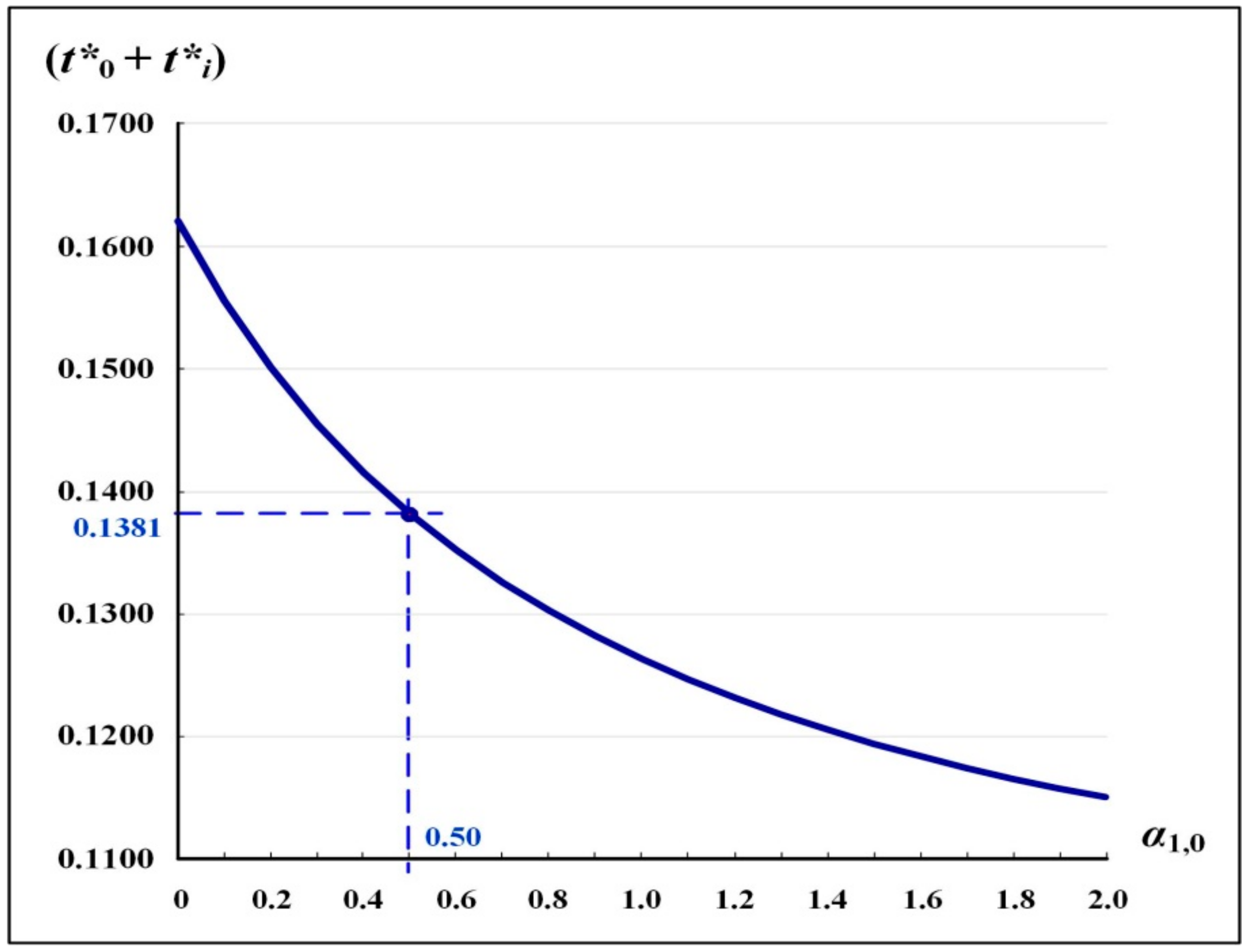
4.1. The Adjustable-Rate Impact on the Uptime and Rework Time and Utilization

Due to the implementation of the expedited production and rework rate for the common parts, its impact on the sum of optimal uptime and rework time of both stages (t₀* + t_i*) is explored, and the result is depicted in Figure 5 and in Table A2 (Appendix A). It indicates that as α_1,0 = 0.5, t₀* declines 32.23% (i.e., from 0.0787 year to 0.0533 year; refer to Table A2) and (t₀* + t_i*) decreases 14.79% (i.e., it drops from 0.1621 to 0.1381; see Figure 5).

Figure 6 illustrates the influence of the adjustable-rate ratio (P_T1,0/P_1,0) on the system’s machine utilization. It shows that the utilization decreases to 0.2485 from 0.2964 (or a decline of 16.18%) due to implementing a 1.5 times standard production rate.

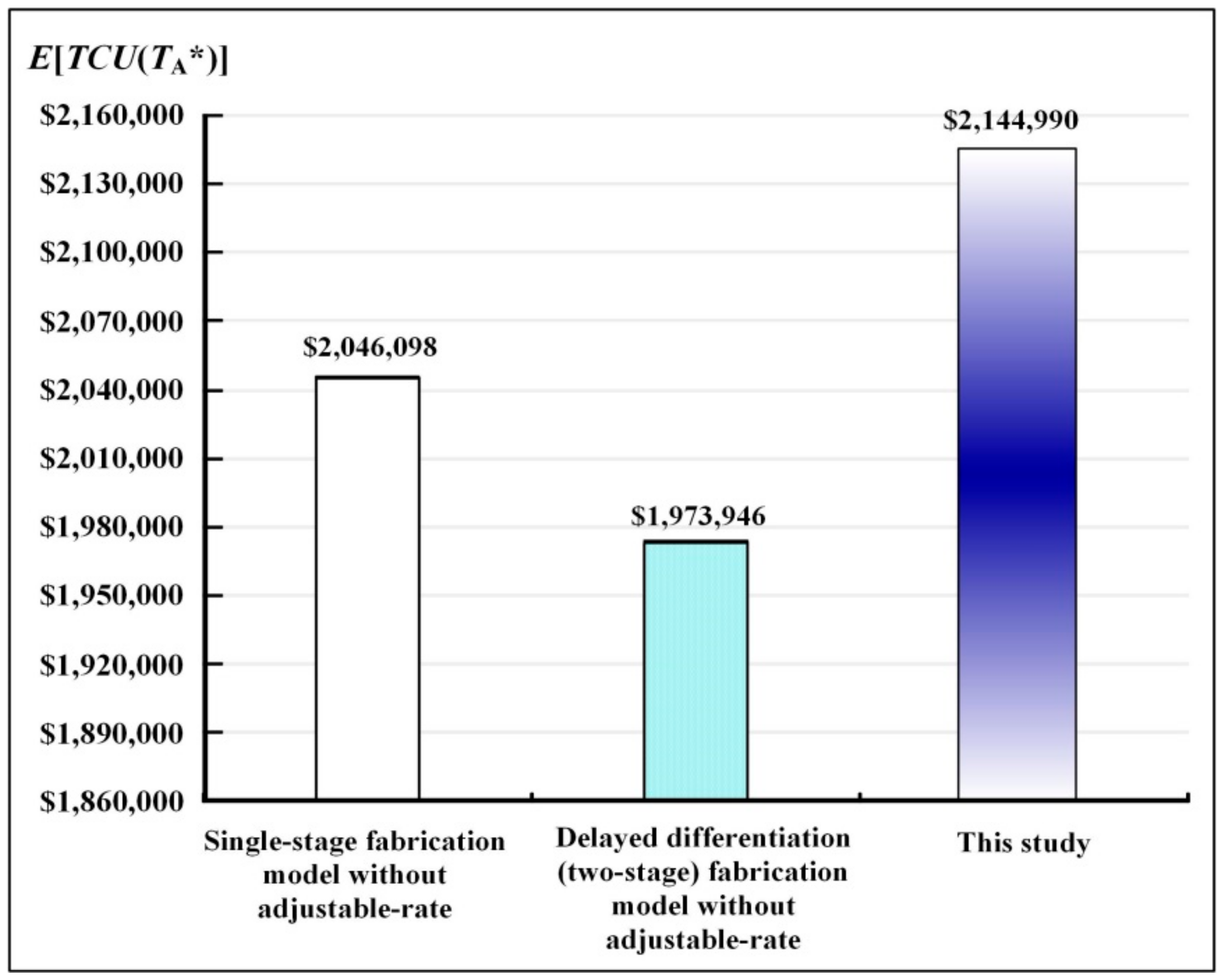
4.2. Comparison of This Work and Other Closely Related Models

We further analyze and compare the utilization and total system cost of this study and closely related models. Figure 7 and Figure 8 illustrate the outcomes, respectively. It indicates that our utilization (i.e., (t₀* + t_i*)/T_A*) is 0.2485 (it drops from 0.2964), or is 16.2% lower than the delayed differentiation model with adjustable-rate (see Figure 7), at the price of an 8.67% increase in cost (i.e., rising from $1,973,946 to $2,144,990; see Figure 8).

Furthermore, as compared to a single-stage fabrication model without adjustable-rate, our model has a 19.89% reduction in utilization (i.e., declining from 0.3102 to 0.2485; see Figure 7), at the price of an 8.67% increase in cost (i.e., rising from $2,046,098 to $2,144,990; see Figure 8).

4.3. The Influence of Other Individual/Collective Features on the System Cost

For the adjustable-rate α_1,0 = 0.5 and the common part’s completion rate γ = 0.5, the breakup of E[TCU(T_A*)] is explicitly analyzed, and the outcomes are displayed in Figure 9. It indicates that common parts’ expedited cost contributes 8.06% to E[TCU(T_A*)] (see Table A2); the sum of rework costs in both stages is 2.29% of E[TCU(T_A*)]; and the sum of setup, holding, and variable costs for end products (stage 2) contribute 56.80% to E[TCU(T_A*)].

Figure 10 demonstrates our model’s capability in analyzing the common part’s linear and nonlinear values (i.e., the factor γ) relating to its completion rate γ. It confirms that our example for the linear value of the common part (i.e., δ = γ¹), and at γ = 0.5, is E[TCU(T_A*)] = $2,144,990. A nonlinear example of the common part value (i.e., δ = γ^1/3) at γ = 0.5 is E[TCU(T_A*)] = $2,201,746.

Each end product’s variable cost regarding α_1,0 is shown in Figure 11. It demonstrates our model’s capability in exploring related performance in the production of end products (in stage 2). It shows that the variable cost for each end product is different, and the variations in α_1,0 have insignificant impacts on these costs.

Figure 12 illustrates the impact adjustable-rate factor on various cost contributors. It exposes that by implementing adjustable-rate α_1,0 = 0.5, E[TCU(T_A*)] increases from $1,973,946 to $2,144,990, a rise of 8.67%. Other relevant cost contributors change slightly as α_1,0 rises.

The collective impact of changes in adjustable-rate α_1,0 and average nonconforming rate on the total system rework cost is illustrated in Figure 13. It exposes that as α_1,0 rises, the total rework cost slightly increases; however, as the average nonconforming rate goes higher, the total rework cost upsurges drastically.

Figure 14 illustrates the collective impact of differences in adjustable-rate α_1,0 and the common part’s completion rate γ on E[TCU(T_A*)]. It reveals that as α_1,0 rises, E[TCU(T_A*)] increases, which upsurges drastically when the γ value is also high. As γ rises, E[TCU(T_A*)] drops slightly when the α_1,0 value is relatively low (less than 0.25), but E[TCU(T_A*)] starts to increase as the α_1,0 value goes beyond 0.25. When both values of γ and α_1,0 are at a high level, E[TCU(T_A*)] upsurges extremely.

5. Conclusions

To respond to customer demand on fast-response, high quality, and diversified goods, we propose a two-stage multiproduct manufacturing scheme that features adjustable-rate, rework, and postponement strategies. We derive the cost-minimized rotation cycle decision through mathematical modeling, formulation, cost analysis, and differential calculus (refer to Section 2 and Section 3). A numerical illustration helps us demonstrate our research results’ applicability, which includes:

(1)

The cost-minimized rotation cycle decision and the convexity of the cost function to the studied model (see Figure 4);

(2)

The adjustable-rate impact on the uptime and rework time, and utilization (refer to Figure 5 and Figure 6) explicitly demonstrates how the adjustable-rate reduces fabrication uptimes and system utilization;

(3)

Comparison of this work and closely related models (see Figure 7 and Figure 8) shows, at a minimal price, how our model’s utilization significantly outperforms that of other models;

(4)

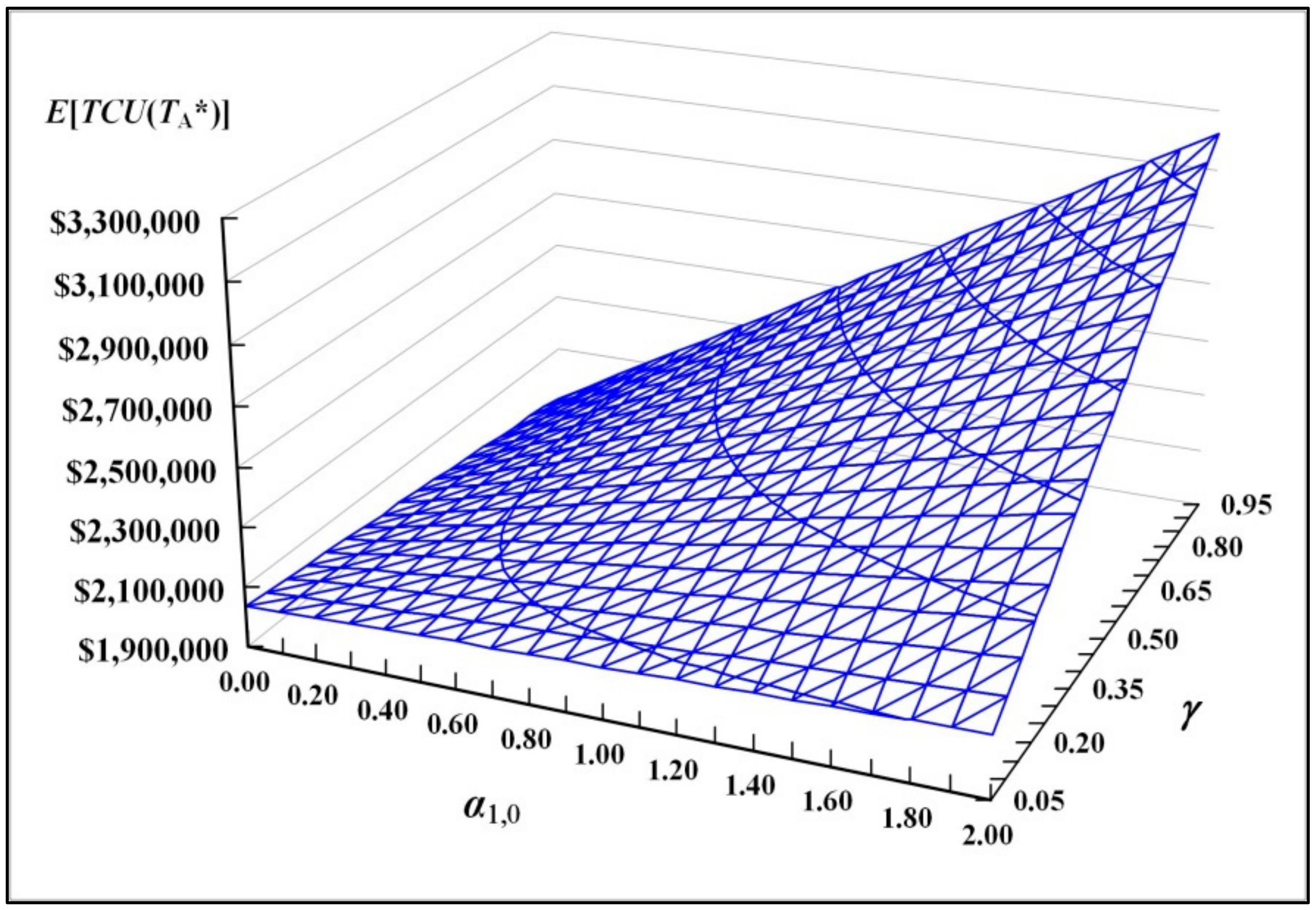
The influence of individual/collective features on the system cost (refer to Figure 9, Figure 10, Figure 11, Figure 12, Figure 13 and Figure 14), such as: (A) Detailed cost contributors to the system cost (see Figure 9); (B) analysis of the impact of the common part’s linear and nonlinear values on system cost (Figure 10); (C) the effect of the adjustable-rate factor on the variable cost for each end-product and system cost (refer to Figure 11 and Figure 12, respectively); (D) the collective impact of adjustable-rate and mean nonconforming rate on the total rework cost (Figure 13); the combined effects of adjustable-rate and common part’s completion rate on the system cost (see Figure 14).

Our decision-support model can offer in-depth managerial insights for manufacturing and operations planning in a wide variety of present-day industries, such as automotive, household merchandise, and clothing. Section 3.4 states the limitation of this study, and additionally, if the demands of multi-item are random variables rather than deterministic, then the proposed model requires a significant revision. When conducting the proposed model, managers can evaluate the tradeoffs between the price paid for implementing the adjustable-rate and the potential benefits gained from utilization decline. For future work, incorporating a multi-delivery plan in the context of this studied problem is a worthy topic to explore.

References

1. Swaminathan, J.M.; Tayur, S.R. Managing design of assembly sequences for product lines that delay product differentiation. IIE Trans. 1999, 31, 1015–1026. [Google Scholar] [CrossRef]
2. Heese, H.S.; Swaminathan, J.M. Product line design with component commonality and cost-reduction effort. Manuf. Serv. Oper. Manag. 2006, 8, 206–219. [Google Scholar] [CrossRef]
3. Ngniatedema, T.; Fono, L.A.; Mbondo, G.D. A delayed product customization cost model with supplier delivery performance. Eur. J. Oper. Res. 2015, 243, 109–119. [Google Scholar] [CrossRef]
4. Granot, D.; Yin, S. Price and order postponement in a decentralized newsvendor model with multiplicative and price-dependent demand. Oper. Res. 2008, 56, 121–139. [Google Scholar] [CrossRef]
5. Bernstein, F.; DeCroix, G.A.; Wang, Y. The impact of demand aggregation through delayed component allocation in an assemble-to-order system. Manag. Sci. 2011, 57, 1154–1171. [Google Scholar] [CrossRef]
6. Chiu, Y.-S.P.; Lin, H.-D.; Wu, M.-F.; Chiu, S.W. Alternative fabrication scheme to study effects of rework of nonconforming products and delayed differentiation on a multiproduct supply-chain system. Int. J. Ind. Eng. Comput. 2018, 9, 235–248. [Google Scholar] [CrossRef]
7. Jabbarzadeh, A.; Haughton, M.; Pourmehdi, F. A robust optimization model for efficient and green supply chain planning with postponement strategy. Int. J. Prod. Econ. 2019, 214, 266–283. [Google Scholar] [CrossRef]
8. Chiu, S.W.; Kuo, J.-S.; Chiu, Y.-S.P.; Chang, H.-H. Production and distribution decisions for a multi-product system with component commonality, postponement strategy and quality assurance using a two-machine scheme. Jordan J. Mech. Ind. Eng. 2019, 13, 105–115. [Google Scholar]
9. Weskamp, C.; Koberstein, A.; Schwartz, F.; Suhl, L.; Voß, S. A two-stage stochastic programming approach for identifying optimal postponement strategies in supply chains with uncertain demand. Omega 2019, 83, 123–138. [Google Scholar] [CrossRef]
10. Tayyab, M.; Sarkar, B.; Ullah, M. Sustainable lot size in a multistage lean-green manufacturing process under uncertainty. Mathematics 2018, 7, 20. [Google Scholar] [CrossRef] [Green Version]
11. Bhuniya, S.; Sarkar, B.; Pareek, S. Multi-product production system with the reduced failure rate and the optimum energy consumption under variable demand. Mathematics 2019, 7, 465. [Google Scholar] [CrossRef] [Green Version]
12. De Kok, A.G. Approximations for operating characteristics in a production-inventory model with variable production rate. Eur. J. Oper. Res. 1987, 29, 286–297. [Google Scholar] [CrossRef]
13. Balkhi, Z.T.; Benkherouf, L. On the optimal replenishment schedule for an inventory system with deteriorating items and time-varying demand and production rates. Comput. Ind. Eng. 1996, 30, 823–829. [Google Scholar] [CrossRef]
14. Giri, B.C.; Dohi, T. Computational aspects of an extended EMQ model with variable production rate. Comput. Oper. Res. 2005, 32, 3143–3161. [Google Scholar] [CrossRef]
15. Ayed, S.; Sofiene, D.; Nidhal, R. Joint optimisation of maintenance and production policies considering random demand and variable production rate. Int. J. Prod. Res. 2012, 50, 6870–6885. [Google Scholar] [CrossRef]
16. Chan, C.K.; Wong, W.H.; Langevin, A.; Lee, Y.C.E. An integrated production-inventory model for deteriorating items with consideration of optimal production rate and deterioration during delivery. Int. J. Prod. Econ. 2017, 189, 1–13. [Google Scholar] [CrossRef]
17. Chiu, Y.-S.P.; Chen, H.-Y.; Chiu, S.W.; Chiu, V. Optimization of an economic production quantity-based system with random scrap and adjustable production rate. J. Appl. Eng. Sci. 2018, 16, 11–18. [Google Scholar]
18. Ameen, W.; AlKahtani, M.; Mohammed, M.K.; Abdulhameed, O.; El-Tamimi, A.M. Investigation of the effect of buffer storage capacity and repair rate on production line efficiency. J. King Saud Univ. Eng. Sci. 2018, 30, 243–249. [Google Scholar] [CrossRef]
19. Chiu, S.W.; Wu, C.-S.; Tseng, C.-T. Incorporating an expedited rate, rework, and a multi-shipment policy into a multi-item stock refilling system. Oper. Res. Persp. 2019, 6, 100115. [Google Scholar] [CrossRef]
20. Palos-Sanchez, P.; Saura, J.R.; Martin-Velicia, F. A study of the effects of programmatic advertising on users’ concerns about privacy overtime. J. Bus. Res. 2019, 96, 61–72. [Google Scholar] [CrossRef]
21. Chiu, S.W.; Huang, Y.-J.; Chiu, Y.-S.P.; Chiu, T. Satisfying multiproduct demand with a FPR-based inventory system featuring expedited rate and scraps. Int. J. Ind. Eng. Comput. 2019, 10, 443–452. [Google Scholar] [CrossRef]
22. Dey, B.K.; Sarkar, B.; Pareek, S. A two-echelon supply chain management with setup time and cost reduction, quality improvement and variable production rate. Mathematics 2019, 7, 328. [Google Scholar] [CrossRef] [Green Version]
23. Lee, H.L. Lot sizing to reduce capacity utilization in a production process with defective items, process corrections, and rework. Manag. Sci. 1992, 38, 1314–1328. [Google Scholar] [CrossRef]
24. Khouja, M. The economic lot and delivery scheduling problem: Common cycle, rework, and variable production rate. IIE Trans. 2000, 32, 715–725. [Google Scholar] [CrossRef]
25. Taleizadeh, A.A.; Wee, H.-M.; Sadjadi, S.J. Multi-product production quantity model with repair failure and partial backordering. Comput. Ind. Eng. 2010, 59, 45–54. [Google Scholar] [CrossRef]
26. Fakher, H.B.; Nourelfath, M.; Gendreau, M. Integrating production, maintenance and quality: A multi-period multi-product profit-maximization model. Reliab. Eng. Syst. Safe. 2018, 170, 191–201. [Google Scholar] [CrossRef]
27. Chiu, S.W.; Liu, C.-J.; Li, Y.-Y.; Chou, C.-L. Manufacturing lot size and product distribution problem with rework, outsourcing and discontinuous inventory distribution policy. Int. J. Eng. Model. 2017, 30, 49–61. [Google Scholar]
28. Rao, A.S.; Singh, A.K. Failure analysis of stainless steel lanyard wire rope. J. Appl. Res. Technol. 2018, 16, 35–40. [Google Scholar] [CrossRef] [Green Version]
29. Wichapa, N.; Khokhajaikiat, P. Solving a multi-objective location routing problem for infectious waste disposal using hybrid goal programming and hybrid genetic algorithm. Int. J. Ind. Eng. Comput. 2018, 9, 75–98. [Google Scholar] [CrossRef]
30. Kore Sudarshan, D.; Vyas, A.K. Impact of fire on mechanical properties of concrete containing marble waste. J. King Saud Univ. Eng. Sci. 2019, 31, 42–51. [Google Scholar] [CrossRef]
31. Larkin, E.V.; Privalov, A.N. Engineering method of fault -tolerant system simulations. J. Appl. Eng. Sci. 2019, 17, 295–303. [Google Scholar] [CrossRef] [Green Version]
32. Ben Fathallah, B.; Saidi, R.; Dakhli, C.; Belhadi, S.; Yallese, M.A. Mathematical modelling and optimization of surface quality and productivity in turning process of aisi 12l14 free-cutting steel. Int. J. Ind. Eng. Comput. 2019, 10, 557–576. [Google Scholar] [CrossRef]
33. Reddy, A.V.; Kumar, B.M. Conditional monitoring of switched reluctance motor for static and dynamic eccentricity faults with fault isolation. Int. J. Math. Eng. Manag. Sci. 2019, 4, 671–682. [Google Scholar] [CrossRef]
34. Kang, C.W.; Ullah, M.; Sarkar, M.; Omair, M.; Sarkar, B. A single-stage manufacturing model with imperfect items, inspections, rework, and planned backorders. Mathematics 2019, 7, 446. [Google Scholar] [CrossRef] [Green Version]
35. Sarkar, B.; Ullah, M.; Choi, S.-B. Joint inventory and pricing policy for an online to offline closed-loop supply chain model with random defective rate and returnable transport items. Mathematics 2019, 7, 497. [Google Scholar] [CrossRef] [Green Version]
36. Bagni, G.; Marçola, J.A. Evaluation of the maturity of the S&OP process for a written materials company: A case study. Gestao Prod. 2019, 26, e2094. [Google Scholar]
37. Romero-Conrado, A.R.; Coronado-Hernandez, J.R.; Rius-Sorolla, G.; García-Sabater, J.P. A Tabu list-based algorithm for capacitated multilevel lot-sizing with alternate bills of materials and co-production environments. Appl. Sci. 2019, 9, 1464. [Google Scholar] [CrossRef] [Green Version]
38. Rius-Sorolla, G.; Maheut, J.; Coronado-Hernandez, J.R.; Garcia-Sabater, J.P. Lagrangian relaxation of the generic materials and operations planning model. Cent. Eur. J. Oper. Res. 2020, 28, 105–123. [Google Scholar] [CrossRef]
39. Nahmias, S. Production & Operations Analysis; McGraw-Hill: New York, NY, USA, 2009. [Google Scholar]
Figure 1. The stock level of the proposed multi-item two-stage postponement model with commonality, adjustable-rate, postponement, and rework as compared to the same system without the implementation of the expedited rate (in grey).
Mathematics 08 01570 g001
Figure 2. A clarified common part’s inventory status during the production process of end product i.
Mathematics 08 01570 g002
Figure 3. The level of nonconforming items of the proposed multi-item two-stage postponement model.
Mathematics 08 01570 g003
Figure 4. The analytical result on the convexity of E[TCU(TA)].
Mathematics 08 01570 g004
Figure 5. The impact of the adjustable-rate on (t0* + ti*).
Mathematics 08 01570 g005
Figure 6. The influence of adjustable-rate ratio (PT1,0/P1,0) on machine utilization.
Mathematics 08 01570 g006
Figure 7. Comparing this study’s utilization with other closely related models.
Mathematics 08 01570 g007
Figure 8. Comparing this study’s E[TCU(TA*)] with other closely related models.
Mathematics 08 01570 g008
Figure 9. The breakup of E[TCU(TA*)].
Mathematics 08 01570 g009
Figure 10. The impact of common part’s linear and nonlinear values on E[TCU(TA*)].
Mathematics 08 01570 g010
Figure 11. Variable production cost for each end product regarding α1,0.
Mathematics 08 01570 g011
Figure 12. The impact of adjustable-rate factor on various cost contributors.
Mathematics 08 01570 g012
Figure 13. The collective impact of changes in α1,0 and average nonconforming rate on total rework cost.
Mathematics 08 01570 g013
Figure 14. The collective impact of differences in α1,0 and γ on E[TCU(TA*)].
Mathematics 08 01570 g014