Eigenloss: Combined PCA-Based Loss Function for Polyp Segmentation

Abstract

Colorectal cancer is one of the leading cancer death causes worldwide, but its early diagnosis highly improves the survival rates. The success of deep learning has also benefited this clinical field. When training a deep learning model, it is optimized based on the selected loss function. In this work, we consider two networks (U-Net and LinkNet) and two backbones (VGG-16 and Densnet121). We analyzed the influence of seven loss functions and used a principal component analysis (PCA) to determine whether the PCA-based decomposition allows for the defining of the coefficients of a non-redundant primal loss function that can outperform the individual loss functions and different linear combinations. The eigenloss is defined as a linear combination of the individual losses using the elements of the eigenvector as coefficients. Empirical results show that the proposed eigenloss improves the general performance of individual loss functions and outperforms other linear combinations when Linknet is used, showing potential for its application in polyp segmentation problems.

1. Introduction

Nowadays, colorectal cancer (CRC) presents high incidence rates in developed countries, as it is mainly considered a lifestyle disease [1]. More than 800,000 deaths are reported yearly and CRC incidence reaches one in ten people worldwide [2]. In 2020, over 104,000 new cases and 53,200 deaths are estimated in the United States alone [3], while more than 174,600 deaths are foreseen in Europe [4]. However, an early detection of CRC, increasing the current 13% up to 50% of patients diagnosed in stage I could save 130,000 lives and reduce the healthcare cost per year by three billion [5]. In this sense, colonoscopy is the gold standard for early diagnosis (CRC screening): the gastroenterologist performs a visual exploration of the rectum and colon using a flexible endoscope inserted through the patient’s anus. During the procedure, polyps are detected and treated if deemed necessary, as these are considered precursor lesions of CRC. Colonoscopy is highly dependent on the endoscopist’s skills, therefore computer-aided diagnosis and detection systems have a great potential to improve clinical results [6].

Recently, deep learning has outperformed classical methods on several computer vision tasks, such as detection, segmentation, classification, and enhancement, also in the healthcare field [7]. The automatic extraction of features performed by convolutional neural networks (CNN) is the main advantage over classical hand-crafted features, but the need of large and annotated datasets is one of its major drawbacks in specific fields, such as medical applications. For this reason, several studies focus on improving the scarce and weak annotations in medical imaging datasets [8]. Although clinical evidence of deep learning algorithms is still poor (there are few studies with low confidence), they show equivalent (or even better) performance than clinicians [9,10]. In this sense, some systematic reviews show the potential of deep learning in gastric tissue diseases [11] and wireless endoscopic capsule [12], but these studies also identify risk of bias due to gaps in the evaluation metrics and public availability of the dataset [11] that must be solved through prospective multicenter studies [12].

In our field of interest, computer-aided detection (CAD) systems have been classically based on the extraction of polyp characteristics, like shape [13], texture [14,15] or depth of valleys [16,17]. Moreover, other classical segmentation methods could be also applied to this problem, such as the alternating direction method of multipliers (ADMM) approach to decompose the image into non-additive components and classify pixels into background and foreground [18] or the approach proposed by Li et al. [19], who combine semi-supervised learning of the posterior class distribution modeled using multinomial logistic regression with segmentation that exploits spatial information. It has been recently determined that up to 80% of missed colonic lesions could be avoided using real-time artificial intelligence assistance [20]. Therefore, there is still a need for further developing polyp detection, localization, and segmentation methods. In this last case, several authors use deep learning methods, which outperform hand-crafted methods [21], and where CNNs are widely used [22]. Among them, the encoder-decoder architectures are a popular family of deep models for semantic segmentation [23]. U-Net [24] is one of the most widely used and well-known architectures for medical imaging segmentation, which has led to many variants for particular applications with great results [25,26,27,28]. While U-Net relies on concatenation in the decoder, LinkNet [29] adds the information from the encoder and has also been used for medical image segmentation [30,31] including polyp segmentation [32]. Furthermore, these two networks are usually compared in studies from different medical fields [33,34,35,36]. For polyp segmentation on colonoscopy images, different approaches can be found. Wichakam et al. [37] proposed a compressed fully convolutional network (FCN) based on VGG-16 [38] which provided state of the art results (Jaccard index of 69.36) while running seven times faster than the original FCN. Vázquez et al. [39] employ a FCN8 architecture [40] and get a Jaccard index equal to 56.07 for the polyp class. Similarly, Wickstrøm et al. [41], also with an enhanced FCN8, get 58.70 overlap.

Principal Component Analysis (PCA) is a mathematical technique for data transformation that reduces multidimensional data sets into a lower number of principal components, which are uncorrelated and retain variance as much as possible [42]. PCA has been used in medical imaging with different purposes. Ansari et al. [43] use the PCA to obtain a target image from a different source image. They transform endoscopic narrow-band images (NBI) into standard colored endoscopic images. In this case, the PCA extracts the fundamental information in NBI, which usually enhances structures and textures, so the standard images can be improved for better assessment and diagnosis. Another application of PCA is the reduction of highly dimensional data, such as fluorescence spectral images of colorectal polyps [44]. In this work, near-infrared autofluorescence spectroscopy images with multiple wavelengths and intensities were obtained from healthy, hyperplastic, and adenomatous colonic tissues and this high dimensional set of images was reduced to eight principal components for an easier and more intuitive tissue classification. It is also worth mentioning that other technical aspects, such as prevention of overfitting in neural networks, have also been addressed with PCA. Kim et al. [45] apply the PCA to reduce the dimensions of the input feature vector while retaining the main information, so the number of weights in the neural network can be reduced. Related to polyp segmentation, PCA has been used as reduction technique for contour region analysis based on hand-crafted features [46].

In statistics, a loss function is commonly used in optimization problems, where the minimum difference between estimated and true values for a given dataset is sought. Therefore, loss functions, also known as objective functions, cost functions, error functions or simply losses, conduct the training process of deep learning models computing the error between predicted values and ground truth and minimizing it to optimize the weights of the model. The relevance and influence of loss functions in deep learning models have been studied in many fields, such as handwritten digits recognition [47], fast single classification [48], cardiac MRI reconstruction [49], low-dose CT images denoising [50], or face recognition [51]. Loss functions can be categorized into distribution, region or boundary-based losses, depending on the main concept considered for minimization. Regarding distribution-based losses, the cross entropy loss function [52] is widely used. It calculates the cost at each pixel using a logarithmic function that is then averaged over all pixels to quantify the difference between the two probability distributions (ground truth vs prediction). Other distributed-based functions are the weight cross entropy [24] and the focal loss [53]. In case of region-based losses, the commonly used Dice loss [25] measures the overlap of two sets, which can be easily applied to binary segmentation. Additional region-based functions are the Jaccard or Intersection over Union (IoU) loss [54], the Tversky loss [55], the Lovász-Hinge or Lovasz-Softmax loss [56], and the focal Tversky loss [57]. Finally, boundary-based loss functions include for example the surface loss that uses a distance metric to compare the shapes of two contours [58], or the loss that uses the estimations of the Hausdorff distance to measure differences between two contours [59].

When deep learning is applied to medical imaging analysis, researchers tend to use classical cross-entropy loss functions together with a second distance or overlap measure [60], so combined loss functions are commonly used [61,62,63]. For polyp segmentation, both individual and combined loss functions can be found. Wichamkam et al. [37] apply the Dice loss function alone. On the other hand, while Zhou [26] combines the Dice loss function with the binary cross entropy, Mohammed et al. [64] combine it with the weight binary cross entropy instead.

Hence, the aim of this paper is to analyze the influence of several loss functions on different models for polyp segmentation and to determine whether a PCA-based decomposition allows for the defining of the coefficients of a non-redundant primal loss function that can outperform the individual loss functions and other aggregation methods, such as the sum and the mean of loss functions. Consequently, the same dataset and training conditions were used for all experiments, while several loss functions were applied to compare the training and testing performance of the model. Two different encoder-decoder architectures, namely U-Net [24] and LinkNet [29], with two backbones each (VGG-16 [40] and Densenet121 [65]) were used for comparison.

The rest of the paper is organized as follows. In Section 2, a detailed description of materials and methods is exposed, including dataset, network architectures, training parameters, loss functions, metrics and PCA analysis. In Section 3, the results are presented and analyzed. Finally, Section 4 discusses the results and Section 5 summarizes the most important conclusions of this work.

2. Materials and Methods

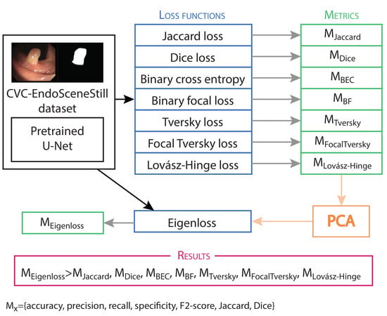
2.1. Dataset

CVC-EndoSceneStill is a publicly available dataset [39] that contains 912 images obtained from 44 video sequences collected from 36 patients. The dataset is divided into training, validation and test sets, each of them including 547, 183, and 182 images, respectively. For each image, binary masks are provided for the polyp, lumen, specular lights and void (black area) classes. In the binary masks, pixels corresponding to the class are labelled with 1, and 0 otherwise (Figure 1). In this work, only the polyp and void classes are used. While the polyp binary mask is used both at training and testing, the void binary mask is just used for reporting metrics with respect to the valid endoscopic image.

2.2. Architectures and Training Parameters

For this study, two backbones (VGG-16 [40] and Densenet121 [65]) and two encoder-decoder architectures (U-Net [24] and LinkNet [29]) were selected. The backbones differ in the type of block used to obtain the feature vector that is fed into the decoder. VGG-16 (Figure 2A) employs convolutional blocks composed of convolutional and activation layers, which are then followed by a max pooling layer to reduce the input size. On the other hand, Densenet121 (Figure 2B) relies on dense blocks where all layers are interconnected with the rest of layers in the block. In both cases, backbones are pretrained using IMAGENET [66], rather than trained from scratch, in order to improve the performance on a small dataset such as CVC-EndosceneStill (only 547 images for training). As for the encoder-decoder architectures, the difference between U-Net and LinkNet mainly lies on the integration of the information of the encoder into the decoder. While U-Net (Figure 2C) concatenates the features maps of the encoder at their corresponding level in the decoder, LinkNet (Figure 2D) adds the input to each encoder layer to the output of the corresponding layer in the decoder. In our implementation, the decoder path is created accordingly to the selected backbone to match the dimensions and number of layers. Therefore, we have four different models (Tables S1–S4 provided in the Supplementary Materials): U-Net-VGG-16 (Figure 2A,C), U-Net-Densenet121 (Figure 2B,C), LinkNet-VGG-16 (Figure 2A,D) and LinkNet-Densenet121 (Figure 2B,D). In all cases, image input size is set to $256\times 256\times 3$ and the predicted binary mask size is $256\times 256\times 1$.

Each model is trained for 300 epochs using the Adam optimizer, a batch size of 16 and batch normalization. The learning rate is initially set to 0.001, decreasing by half every 5 epochs and restoring the initial value every 25 epochs. The weights of the best epoch (lowest validation loss) are used for prediction. All experiments were implemented using segmentation models [67], Keras [68] and Tensorflow [69] as backend and were run in a NVIDIA Quadro P5000 with 16 GB memory.

2.3. Loss functions

Seven loss functions are considered in this work. In order to present their formulation, we firstly establish the mathematical framework of the binary segmentation problem. Since we are performing a binary semantic segmentation based on a pixel-wise classification, we describe the problem of a binary classifier.

As $\mathit{X}$ is the image of size M × N to be segmented, each pixel $x\in \mathit{X}$ has a corresponding value, $y$, in the ground truth mask, $\mathit{Y}$. In a binary classification problem, the ground truth labels can take the values $y=\left\{y_1,y_0\right\}$, where $y_1$ is the positive class, being polyp in this case, and $y_0$ the negative class, corresponding to the background class. The segmentation model gives a prediction $\widehat{\mathit{Y}}$, with labels $\widehat{y}=\left\{{\widehat{y}}_1,{\widehat{y}}_0\right\}$. In our work, labels are assigned as $y_1=1; y_0=0; {\widehat{y}}_1=1; {\widehat{y}}_0=0$. Thus, the elements of the confusion matrix, $n_{ij}$, indicate the number of cases belonging to class i that were classified as class j. In our binary problem, the elements of the 2 × 2 confusion matrix are:

• $n_{11}$, or true positives (TP): polyp pixels in the ground truth binary mask that are correctly classified as polyp in the predicted binary mask.
• $n_{10}$, or false negatives (FN): polyp pixels in the ground truth binary mask that are incorrectly classified as background in the predicted binary mask.
• $n_{01}$, or false positives (FP): background pixels in the ground truth binary mask that are incorrectly classified as polyp in the predicted binary mask.
• $n_{00}$, or true negatives (TN): background pixels in the ground truth binary mask that are correctly classified as background in the predicted binary mask.

Therefore, any loss function $L\left(Y,\widehat{\mathit{Y}}\right)$ measures the cost or error of predicting $\widehat{\mathit{Y}}$ for a given image $\mathit{X}$ with ground truth $\mathit{Y}$ [70]. In the following subsections, we define the loss functions considered in this study.

2.3.1. Jaccard Loss

The Jaccard index [71], also known as intersection over union (IoU), provides the ratio of the intersection between the ground truth and the predicted binary masks over their union, in a [0, 1] range and with the convention of solving the indetermination $0/0=1$. In our particular dataset, this situation does not occur as all images contains a segmented polyp, so the ground truth binary masks always contain positive elements. Based on this index, the Jaccard loss can be defined as:

$$L_{Jaccard}\left(\mathit{Y},\widehat{\mathit{Y}}\right)=1-\frac{\left|\mathit{Y}{{\displaystyle \cap }}^{ }\widehat{\mathit{Y}}\right|}{\left|\mathit{Y}{{\displaystyle \cup }}^{ }\widehat{\mathit{Y}}\right|}=1-\frac{{\sum }_{i=1}^{M·N}{y}_i·{\widehat{y}}_i}{{\sum }_{i=1}^{M·N}{y}_i+{\sum }_{i=1}^{M·N}{\widehat{y}}_i-{\sum }_{i=1}^{M·N}{y}_i·{\widehat{y}}_i}=1-\frac{TP}{TP+FN+FP}$$

(1)

This loss function is widely used in segmentation problems as it directly optimizes the Jaccard index, one of the most common metrics.

2.3.2. Dice Loss

The Dice coefficient [72] also measures similarities between two regions. This coefficient is the same as the F1-score. The Dice loss can be defined as:

$$L_{Dice}\left(\mathit{Y},\widehat{\mathit{Y}}\right)=1-\frac{\mathsf{2}·\left|\mathit{Y}{{\displaystyle \cap }}^{ }\widehat{\mathit{Y}}\right|}{\left|\mathit{Y}\right|+\left|\widehat{\mathit{Y}}\right|}=1-\frac{2{\sum }_{i=1}^{M·N}{y}_i·{\widehat{y}}_i}{{\sum }_{i=1}^{M·N}{y}_i+{\sum }_{i=1}^{M·N}{\widehat{y}}_i}=1-\frac{2·TP}{2·TP+FN+FP}$$

(2)

2.3.3. Binary Cross Entropy Loss

Cross entropy or softmax loss is the most widely used loss function for classification problems [73]. For a binary classification problem, binary cross entropy can be defined as:

$$L_{BEC}\left(\mathit{Y},\widehat{\mathit{Y}}\right)=\frac{1}{M·N}{\displaystyle \sum }_{\mathrm{i}=1}^{M·N}\left(-y_i·\log \left(\widehat{y_i}\right)-\left(1-y_i\right)·\log \left(1-{\widehat{y}}_i\right)\right)$$

(3)

The aim of this distributed-based loss function is to maximize the accuracy of the predicted binary mask, considering both the positive class, or polyp, and the negative class, or background.

2.3.4. Binary Focal Loss

Yin et al. [53] defined the focal loss to counteract the effect of imbalanced classes. For a binary problem, it can be defined as:

$$L_{BF}\left(\mathit{Y},\widehat{\mathit{Y}}\right)={\displaystyle \sum }_{\mathrm{i}=1}^{M·N}(-y_i·\propto ·{\left(1-{\widehat{y}}_i\right)}^{\gamma }·\log \left({\widehat{y}}_i\right)-\left(1-y_i\right)·\propto ·{\widehat{y}}_i{}^{\gamma }·log(1-{\widehat{y}}_i))$$

(4)

being $\alpha$ a weighting factor in balanced cross entropy and $\gamma$ a focusing parameter. We have considered $\alpha =0.25$ and $\gamma =2.0$, default parameters in the segmentation models library [67].

2.3.5. Tversky Loss

The Tversky index [74] allows us to control the penalties for FP and FN through the parameters $\alpha$ and $\beta$, and it is defined as:

$$TI\left(\mathit{Y},\widehat{\mathit{Y}}\right)=\frac{{\sum }_{i=1}^{M·N}{y}_{pi}{\widehat{y}}_{pi}+ϵ}{{\sum }_{i=1}^{M·N}{y}_{pi}{\widehat{y}}_{pi}+\alpha {\sum }_{i=1}^{M·N}{y}_{ip}{\widehat{y}}_{i\overline{p}}+\beta {\sum }_{i=1}^{M·N}{y}_{i\overline{p}}{\widehat{y}}_{ip}+ϵ}$$

(5)

where p stands for the polyp class, so $y_{pi}=1$ if pixel i belongs to the polyp class, and 0 otherwise, and the opposite for $y_{\overline{p}i}$ in the ground truth binary mask. The same definitions apply for ${\widehat{y}}_{pi}$ and ${\widehat{y}}_{\overline{p}i}$ in the predicted binary mask. Based on this index, the Tversky loss function is defined as:

$$L_{Tversky}\left(\mathit{Y},\widehat{\mathit{Y}}\right)=1-TI\left(\mathit{Y},\widehat{\mathit{Y}}\right)$$

(6)

For implementation, we have selected $\alpha =0.7$ and $\beta =1-\alpha =0.3$, as the authors report in their original work.

2.3.6. Focal Tversky Loss

Based on the Tversky index (Equation (6)) and combining the idea of the binary focal loss (Section 2.3.4), Abraham et al. [57] defined the Focal Tversky loss as:

$$L_{FocalTversky}\left(\mathit{Y},\widehat{\mathit{Y}}\right)={\left(1-TI\left(\mathit{Y},\widehat{\mathit{Y}}\right)\right)}^{\raisebox{1ex}{$1$}\!\left/ \!\raisebox{-1ex}{$\gamma $}\right.}$$

(7)

to address the issue of data imbalance in medical imaging segmentation. For implementation, we have selected $\gamma =\frac{4}{3}$, as the authors report in their original work.

2.3.7. Lovász-Hinge Loss

Berman et al. [56] propose the Lovász-Hinge loss function, based on the convex Lovász extension of sub-modular losses. For our binary problem, it is defined as:

$$L_{Lovász-Hinge}\left(\mathit{Y},\widehat{\mathit{Y}}\right)=\overline{{\mathsf{\Delta }}_{J_p}}\left(\mathit{m}\left(p\right)\right)$$

(8)

where $\overline{{\mathsf{\Delta }}_{J_p}}$ is the Lovász extension to the Jaccard loss function and $\mathit{m}\left(p\right)$ is the vector of hinge losses for the polyp class, as defined in [56].

2.4. Metrics

The results are always reported over the 182 images of the test set of CVC-EndoSceneStill dataset, which allows for a fair comparison of the models. To calculate the reporting metrics, only the valid area of the void binary mask (Figure 1c) is considered. For each image, seven metrics are calculated based on the elements of the confusion matrix:

$$Accuracy=\frac{TP+TN}{TP+TN+FP+FN}$$

(9)

$$Precision=\frac{TP}{TP+FP}$$

(10)

$$Recall=\frac{TP}{TP+FN}$$

(11)

$$Specificity=\frac{TN}{TN+FP}$$

(12)

$$F2-score=\frac{5·TP}{5·TP+4·FN+FP}$$

(13)

$$Jaccard=\frac{TP}{TP+FN+FP}$$

(14)

$$Dice=\frac{2·TP}{2·TP+FN+FP}$$

(15)

2.5. PCA Analysis

Previously to the application of the PCA, the viability of the method was tested. Therefore, the existing correlation between the variables under study was determined based on the correlation matrix and two statistical tests: Kaiser-Meyer-Olkin (KMO) index and χ² test. Next, the Bartlett sphericity test was carried out to determine the correlation between all variables. This test is based on Pearson’s χ² distribution, indicating that a significant correlation between variables other than zero when the determinant of the correlation matrix is different from one. The mean of the KMO sample fit was also calculated to measure the proportion of variance that the variables under study have in common. This parameter ranges from 0 to 1, considering a good sample suitability to use PCA for values greater than 0.5.

Under the assumption that these tests are positive, a PCA was performed using the seven metrics of the 182 images of the test set predicted by the model trained with each individual loss function, in order to identify non-correlated variables that allow for a dimensionality reduction while the included variance is maximized. We have a set of data $X\in {ℝ}^{N\times D}$, where N is the number of metrics calculated for the 182 images of the test set and D is the number of loss functions. The objective is to project $X$ into Y$\in {ℝ}^{N\times K}$, where $K<D$, while maximizing the variance included in $Y$. If the $D$ variables are correlated, the information in $X$ is redundant, so the PCA analysis allows for a dimension reduction resulting in a set of independent variables. For that, eigenvectors and eigenvalues from the correlation matrix are calculated. Eigenvalues are sorted in descending order and $K$ eigenvectors with the largest eigenvalues are selected. Then, the original dataset $X$ can be transformed into Y using the projection matrix $\mathit{W}$ from the selected $K$ eigenvectors as:

$$Y=\mathit{W}X={\alpha }_{k1}{X}_1+{\alpha }_{k2}{X}_2+\dots +{\alpha }_{KN}{X}_N$$

(16)

being ${\alpha }_{kn}$ the coefficient of the k-th principal component for the n-th input variable. The resulting components were examined and only those with eigenvalues greater than 1 which also include a great proportion of variance (over 80%) were considered [75]. We can define an eigenloss function for each principal component as a linear combination of the individual loss functions as:

$$\begin{array}{cc}\hfill L_{k Eigenloss}\left(\mathit{Y},\widehat{\mathit{Y}}\right)=& {\alpha }_{k Jaccard}·L_{Jaccard}\left(\mathit{Y},\widehat{\mathit{Y}}\right)+{\alpha }_{k Dice}·L_{Dice}\left(\mathit{Y},\widehat{\mathit{Y}}\right)+{\alpha }_{k BCE}\hfill \\ & ·L_{BCE}\left(\mathit{Y},\widehat{\mathit{Y}}\right)+{\alpha }_{k BF}·L_{BF}\left(\mathit{Y},\widehat{\mathit{Y}}\right)+{\alpha }_{k Tversky}·L_{Tversky}\left(\mathit{Y},\widehat{\mathit{Y}}\right)\hfill \\ & +{\alpha }_{k FocalTversky}·L_{FocalTversky}\left(\mathit{Y},\widehat{\mathit{Y}}\right)+{\alpha }_{k Lovasz Hinge}\hfill \\ & ·L_{Lovasz Hinge}\left(\mathit{Y},\widehat{\mathit{Y}}\right)\hfill \end{array}$$

(17)

3. Results and Analysis

3.1. PCA Analysis

Table 1. U-Net-VGG-16. Results of the model trained with the different loss functions, reported over the test set of CVC-EndoSceneStill. Best values are indicated in bold.

Loss Function	Accuracy	Precision	Recall	Specificity	F2-Score	Jaccard	Dice
Jaccard	93.36 ± 10.26	88.69 ± 23.02	65.65 ± 37.52	99.24 ± 1.73	65.79 ± 36.20	59.77 ± 35.03	67.39 ± 34.44
Dice	92.76 ± 10.45	82.20 ± 27.36	63.24 ± 37.94	99.07 ± 1.66	63.23 ± 36.42	56.38 ± 34.59	64.61 ± 34.47
Binary entropy	93.18 ± 10.28	85.39 ± 30.95	64.62 ± 38.92	99.29 ± 1.45	64.89 ± 37.90	59.48 ± 36.35	66.39 ± 36.58
Binary focal	93.34 ± 10.28	82.44 ± 26.45	68.84 ± 36.37	98.59 ± 2.84	68.13 ± 34.91	60.49 ± 33.66	68.48 ± 33.59
Tversky	92.80 ± 10.53	82.80 ± 29.18	60.84 ± 39.16	99.22 ± 1.57	61.20 ± 38.03	55.34 ± 36.12	62.88 ± 36.59
Focal Tversky	93.10 ± 9.94	81.19 ± 26.54	64.03 ± 38.72	98.98 ± 2.13	63.81 ± 37.25	57.20 ± 35.57	64.89 ± 35.46
Lovász-Hinge	91.26 ± 11.07	72.26 ± 41.71	40.09 ± 39.55	99.71 ± 0.86	41.48 ± 39.44	38.23 ± 37.64	44.74 ± 39.49
Sum	92.78 ± 10.45	81.15 ± 32.97	57.76 ± 39.88	99.37 ± 1.44	58.43 ± 39.01	53.58 ± 37.44	60.64 ± 38.11
Mean	93.33 ± 10.5	84.07 ± 29.03	69.53 ± 35.64	98.84 ± 2.42	69.38 ± 34.42	62.83 ± 33.45	70.49 ± 33.13
Eigenloss	93.00 ± 10.91	80.31 ± 31.35	65.07 ± 37.70	99.00 ± 2.25	65.45 ± 36.70	59.66 ± 35.32	67.04 ± 35.39
Norm Eigenloss	92.97 ± 10.13	81.62 ± 27.02	64.02 ± 37.73	98.91 ± 2.06	63.82 ± 35.99	56.56 ± 33.99	65.01 ± 33.99

,

Table 2. U-Net-Densenet121. Results of the model trained with the different loss functions, reported over the test set of CVC-EndoSceneStill. Best values are indicated in bold.

Loss Function	Accuracy	Precision	Recall	Specificity	F2-Score	Jaccard	Dice
Jaccard	95.02 ± 9.53	86.95 ± 23.58	79.18 ± 33.08	99.14 ± 1.66	78.56 ± 31.94	72.17 ± 31.06	78.45 ± 30.37
Dice	94.17 ± 10.22	90.10 ± 24.86	77.88 ± 33.74	98.99 ± 2.34	76.63 ± 32.63	69.88 ± 32.63	76.30 ± 31.61
Binary entropy	94.30 ± 9.68	86.58 ± 23.06	75.60 ± 33.75	99.12 ± 1.65	74.96 ± 32.17	68.07 ± 31.89	75.39 ± 30.06
Binary focal	94.27 ± 9.81	84.61 ± 22.94	80.84 ± 31.62	98.64 ± 2.67	78.69 ± 30.03	70.01 ± 30.18	77.40 ± 28.41
Tversky	94.74 ± 9.77	89.04 ± 19.81	81.04 ± 30.35	99.02 ± 2.29	79.71 ± 29.35	73.19 ± 30.17	79.72 ± 27.98
Focal Tversky	94.19 ± 9.83	83.08 ± 25.12	78.59 ± 34.18	98.62 ± 2.90	68.05 ± 32.22	75.10 ± 31.24	79.84 ± 24.73
Lovász-Hinge	94.73 ± 9.77	87.52 ± 21.59	80.07 ± 31.72	98.95 ± 2.37	79.01 ± 30.42	72.26 ± 30.62	78.86 ± 28.78
Sum	94.76 ± 9.53	87.92 ± 22.08	80.72 ± 30.32	98.95 ± 2.38	79.69 ± 29.12	72.89 ± 29.77	79.62 ± 27.80
Mean	94.45 ± 9.77	86.12 ± 22.40	80.45 ± 31.49	98.82 ± 2.56	78.48 ± 30.17	70.75 ± 30.84	77.72 ± 28.96
Eigenloss	94.43 ± 9.78	89.83 ± 21.63	77.39 ± 33.28	99.06 ± 2.18	76.41 ± 31.97	69.35 ± 31.55	76.33 ± 30.39
Norm Eigenloss	94.68 ± 9.69	87.85 ± 22.12	79.24 ± 32.31	99.09 ± 1.95	78.43 ± 31.11	71.86 ± 31.02	78.37 ± 29.60

,

Table 3. LinkNet-VGG-16. Results of the model trained with the different loss functions, reported over the test set of CVC-EndoSceneStill. Best values are indicated in bold.

Loss Function	Accuracy	Precision	Recall	Specificity	F2-Score	Jaccard	Dice
Jaccard	93.41 ± 10.47	82.86 ± 30.16	68.2 ± 36.67	99.34 ± 1.22	68.51 ± 35.56	62.75 ± 34.19	70.07 ± 34.11
Dice	93.59 ± 10.38	81.03 ± 32.94	67.58 ± 38.01	99.49 ± 0.96	67.90 ± 37.10	62.53 ± 35.45	69.24 ± 35.92
Binary entropy	93.61 ± 9.98	83.01 ± 26.67	70.18 ± 35.97	98.97 ± 1.97	69.76 ± 34.50	62.65 ± 33.05	70.48 ± 32.88
Binary focal	93.15 ± 10.28	81.04 ± 28.02	66.18 ± 38.02	98.95 ± 1.76	65.63 ± 36.44	58.36 ± 34.85	66.22 ± 34.65
Tversky	93.45 ± 10.78	82.54 ± 28.10	69.82 ± 37.05	99.13 ± 1.85	69.55 ± 35.85	63.14 ± 34.49	70.27 ± 34.33
Focal Tversky	93.56 ± 10.35	83.56 ± 26.75	70.18 ± 37.39	99.09 ± 1.74	69.54 ± 36.10	62.81 ± 34.66	69.91 ± 34.58
Lovász-Hinge	92.98 ± 10.28	80.57 ± 29.84	68.17 ± 37.82	98.73 ± 2.60	67.21 ± 36.06	59.6 ± 34.49	67.42 ± 34.23
Sum	93.26 ± 10.08	78.00 ± 32.57	68.06 ± 36.90	98.76 ± 2.59	67.53 ± 35.50	60.4 ± 34.20	68.17 ± 34.12
Mean	93.53 ± 10.36	84.11 ± 28.24	68.64 ± 37.03	99.35 ± 1.23	68.80 ± 35.79	62.77 ± 34.16	70.10 ± 34.05
Eigenloss	93.50 ± 10.60	83.31 ± 28.49	69.52 ± 36.50	99.28 ± 1.76	69.51 ± 35.31	63.24 ± 33.86	70.61 ± 33.68
Norm Eigenloss	93.12 ± 10.59	84.35 ± 28.65	65.74 ± 37.70	99.33 ± 1.61	66.13 ± 36.53	60.62 ± 35.21	67.93 ± 35.03

and

Table 4. LinkNet-Densenet121. Results of the model trained with the different loss functions, reported over the test set of CVC-EndoSceneStill. Best values are indicated in bold.

Loss Function	Accuracy	Precision	Recall	Specificity	F2-Score	Jaccard	Dice
Jaccard	94.71 ± 9.08	87.32 ± 20.08	81.92 ± 27.25	98.58 ± 3.05	79.84 ± 26.01	71.57 ± 28.02	79.44 ± 24.79
Dice	94.47 ± 9.90	86.44 ± 23.22	76.91 ± 34.45	99.19 ± 1.52	76.27 ± 33.16	69.71 ± 32.18	76.32 ± 31.22
Binary entropy	93.99 ± 10.18	84.52 ± 25.45	77.44 ± 34.21	98.70 ± 2.73	75.96 ± 32.98	68.74 ± 32.73	75.44 ± 31.57
Binary focal	94.39 ± 9.88	85.15 ± 25.81	77.04 ± 34.42	99.08 ± 2.07	75.99 ± 33.15	69.11 ± 32.62	75.71 ± 31.76
Tversky	94.68 ± 9.41	88.13 ± 21.48	78.47 ± 31.38	99.00 ± 2.37	77.74 ± 29.93	70.92 ± 30.11	78.12 ± 28.08
Focal Tversky	94.31 ± 9.64	85.96 ± 21.48	81.01 ± 29.48	98.52 ± 3.11	79.16 ± 27.99	70.84 ± 28.83	78.53 ± 26.54
Lovász-Hinge	94.89 ± 9.56	86.73 ± 22.64	79.62 ± 31.09	99.21 ± 1.29	79.02 ± 30.08	72.41 ± 29.88	79.13 ± 28.59
Sum	94.36 ± 9.65	84.13 ± 25.73	76.50 ± 34.19	99.01 ± 1.67	75.47 ± 32.69	68.36 ± 32.11	75.45 ± 30.70
Mean	94.11 ± 10.09	85.48 ± 26.24	74.92 ± 34.48	98.96 ± 2.67	74.17 ± 33.11	67.77 ± 32.82	74.7 ± 31.61
Eigenloss	94.59 ± 9.61	88.65 ± 18.25	80.23 ± 30.78	99.05 ± 1.92	79.18 ± 29.26	71.84 ± 29.25	79.07 ± 27.07
NormEigenloss	94.60 ± 9.86	87.79 ± 21.65	77.81 ± 32.85	99.16 ± 1.89	77.49 ± 31.66	71.57 ± 31.28	78.06 ± 29.85

summarize the results of the different models in the test set of CVC-EndoSceneStill. Metrics calculated in the [0, 1] range were transformed into [0, 100] range for better visualization. In all models, the accuracy is always closer to 100 due to the influence of the background in this metric and the unbalance between polyp and background classes. This is also found in the case of precision and specificity, where values are in general over 80.00 and 98.00, respectively. On the contrary, recall, F2-score, Jaccard and Dice provide lower values, ranging from around 40.00 to 81.00. It is important to highlight the small deviation of the specificity in comparison to the rest of the metrics. This is due to the high presence of background pixels, which makes the TN a very stable figure. When classes are highly unbalance, such as our case because the polyp represents 12.50 ± 11.49% (range: 0.75–66.15) of the image, metrics that do not consider the TN (precision, recall, F2-score, Jaccard and Dice) are more representative of the performance.

At loss function level, the Jaccard and Tversky losses appear to provide the most stable results along the different models. On the contrary, the binary cross entropy, the binary focal and the Lovász-Hinge loss functions provide different results depending on the model. On the other hand, models with the Densenet121 backbone obtain overall better results than models using VGG-16 for all individual loss functions. Using U-Net (concatenation) or LinkNet (add) lead to similar results for the individual loss functions.

Figure 2 and Figure 3 show the boxplots for the accuracy and Jaccard index for the four models. Boxplots for the rest of metrics are provided as Supplementary Materials (Figures S1–S5). While the accuracy is more similar for all loss functions and models, the Jaccard index presents a greater variability and differences among them.

The correlation matrix presents high values ranging from 0.659 to 0.898 outside the main diagonal of the matrix for the four analyzed models. Therefore, correlation between the variables under study can be considered high and significant (p-value ≤ 0.001 in all cases). Furthermore, the value of the determinant of the correlation matrix was 0 for each model, so there is a linear relationship between the variables under study. Next, for the Bartlett sphericity test value, we obtain a χ² greater than 10,000 which indicates that there are high values outside the diagonal of the correlation matrix with significance less than 0.001, for all models. In the KMO sample fit, the value ranged from 0.937 to 0.941 for the four models, which corroborates the results of the previous statistical parameters. Therefore, we can conclude that the PCA can be applied to the variables under study in the four models.

The PCA analysis identified only one independent component for each considered model (

Table 5. PCA results. Com: Communality; ${\alpha }_{1n}$

	U-Net-VGG-16		U-Net-Densenet121		LinkNet-VGG-16		LinkNet-Densenet121
Eigenvalue	5.803		6.076		5.913		5.998
% Variance	82.91		86.80		84.47		85.69
Loss function	Com.	${\alpha }_{1n}$	Com.	${\alpha }_{1n}$	Com.	${\alpha }_{1n}$	Com.	${\alpha }_{1n}$
Jaccard	0.875	0.935	0.819	0.905	0.843	0.918	0.819	0.905
Dice	0.845	0.919	0.894	0.946	0.864	0.930	0.878	0.937
Binary cross entropy	0.835	0.914	0.785	0.886	0.866	0.930	0.842	0.918
Binary focal	0.826	0.909	0.892	0.944	0.805	0.897	0.861	0.928
Tversky	0.881	0.939	0.906	0.952	0.842	0.917	0.881	0.939
Focal Tversky	0.884	0.940	0.869	0.932	0.888	0.942	0.878	0.937
Lovász-Hinge	0.657	0.811	0.911	0.954	0.805	0.897	0.840	0.916

).

Based on these results, the eigenloss was calculated using the coefficients of the first principal component, ${\alpha }_{1n}$, from Table 5 in (Equation (17)) for each considered model. Results for the test set of the models trained with its corresponding eigenloss are provided in the penultimate row of Table 1, Table 2, Table 3 and Table 4, as well as in the penultimate boxes of Figure 3 and Figure 4. For comparison, we also analyzed other linear combinations:

• Sum: where all coefficients are equal to 1.
• Mean: where all coefficients are equal to $1/7$.
• Normalized eigenloss: where coefficients ${\alpha }_{1n}$ are normalized using the formula.

  $${\alpha }_{1n}^{\prime }=\frac{{\alpha }_{1n}}{{\sum }_n{\alpha }_{1n}}$$

  (18)

  with $n\in \left\{Jaccard, Dice, BCE,BF,Tversky,FocalTversky, Lovasz-Hinge\right\}.$

The proposed eigenloss improves the general performance of individual loss functions in all models, as it provides closer values to 100 in the seven metrics at the same time, although the maximum value might be for any of the individual losses. It is interesting to remark that the F2-score of the combined loss function improves, therefore providing a better balance between precision and recall than the individual loss functions. Our proposed combination also minimizes variability in the Jaccard index.

In comparison to other linear combinations, the eigenloss obtains better results than the sum and the mean when LinkNet architecture is considered, regardless of the backbone. On the other hand, for the U-Net, either the sum or the mean performs better.

3.2. Training and Testing Analysis

Table 6. Best epoch (# Epoch) and value of the validation loss (Val Loss) for each model and loss function.

	U-Net-VGG-16		U-Net-Densenet121		LinkNet-VGG-16		LinkNet-Densenet121
Loss Function	# Epoch	Val Loss	# Epoch	Val Loss	# Epoch	Val Loss	# Epoch	Val Loss
Jaccard	292	0.17	71	0.16	292	0.18	17	0.15
Dice	216	0.19	71	0.12	211	0.17	71	0.16
Binary cross entropy	292	0.16	71	0.15	292	0.15	211	0.14
Binary focal	198	0.20	153	0.19	292	0.15	17	0.16
Tversky	292	0.16	71	0.16	292	0.18	47	0.18
Focal Tversky	216	0.20	71	0.14	292	0.16	211	0.17
Lovász-Hinge	184	0.19	71	0.15	216	0.16	17	0.16
Sum	259	0.22	71	0.15	292	0.18	128	0.15
Mean	172	0.16	71	0.14	211	0.12	17	0.14
Eigenloss	211	0.19	114	0.17	211	0.14	17	0.16
Normalized eigenloss	211	0.20	71	0.13	292	0.16	17	0.18

summarizes the best epoch and the corresponding validation loss at which weights are selected for prediction as indicated in Section 2.2.

Models with VGG-16 converge slower, the lowest epoch is 172 and 211 for the U-Net-VGG-16 and LinkNet-VGG-16, respectively. On the other hand, LinkNet-Densenet121 converges faster than U-Net-Densenet121 for most losses. In general, all loss values in the best epochs are quite similar, ranging from 0.12 to 0.20. These findings are also observable in Figures S6–S9 included as Supplementary Materials. They show the evolution of the losses during training for the training and validation sets. Peaks are produced when the learning rate is restored to its initial value.

Although there are no great differences in the initial convergence within each model, largest differences are obtained in LinkNet-VGG-16, where Lovász-Hinge is the slowest one and the binary cross entropy the fastest one among the individual loss functions (Figure 5). In all cases, the general trend of the eigenloss is to run within the maximum and minimum values set by the individual loss functions.

Figures S10–S13 provided in the Supplementary Materials show the evolution of the loss, accuracy and Jaccard index during training for the training and validation sets for each model and each loss function. In all cases, accuracy values for train and validation sets remain very similar from the first epochs, achieving values very close to 100. This is due to fact that the background class is considered in the accuracy, so even when the polyp is not detected at all, accuracy is still high thanks to the negative class. Therefore, accuracy is not the most suitable metric for polyp segmentation. On the other hand, Jaccard index values in training and validation set vary along the whole training for all models and loss functions. Moreover, it shows greater fluctuations, showing a more erratic behavior when VGG-16 is used as backbone. As it might be expected, Jaccard and Dice losses provide a more stable value for the Jaccard index during training for the training and validation set, as the metric is either directly or indirectly included in the loss function for optimization. The proposed eigenloss remains acceptably stable during training, reaching values around 60 in the best epoch.

4. Discussion

Computer-aided detection systems have the potential to improve colonoscopy [6]. In this way, polyps, considered early precursors of CRC, can be detected, diagnosed and treated. In this work, we have faced the problem of polyp detection by the application of segmentation models based on deep learning. Specifically, we have analyzed the influence of seven loss functions on four models for polyp segmentation and determined whether a PCA-based decomposition allows for the defining of a non-redundant primal loss function that can outperform them and different linear combinations.

Through the application of PCA, the eigenloss was defined as a linear combination of seven individual loss functions. It does improve overall performance over the individual loss functions for the four considered models. On the other hand, and only for the LinkNet architecture, the eigenloss performs better than the sum and the mean. Regarding the backbones, the eigenlos performs better with the Densenet121 than VGG-16, in all cases. This might be due to the fact that VGG-16 presents a more linear architecture that cannot extract enough details for segmenting complex structures such as the polyp, due to the high level of visual similarity between healthy mucosa and lesion. Furthermore, it is also worth mentioning that the eigenloss provides the most balanced results in terms of precision and recall, therefore balancing false positives and false negatives.

Based on the experimental results of the individual loss functions, region-based loss functions provide better results for polyp segmentation. While highest values remain in the individual loss functions in many cases, the eigenloss improves the overall performance providing a more balanced result among all metrics for each model. Therefore, one benefit of using the eigenloss is to include the properties of both region and distribution-based loss functions in one single loss function, which might be the reason for this balanced behavior, which arises from the PCA capability for projecting the existing losses into a statistically independent eigenloss. This way, there is no need for choosing one over the other, except in the case that one loss function behaves outstandingly well in all metrics. Due to the fact that PCA provides a compression with information loss, the use of the eigenloss in this case might hinder the performance if the individual loss function is used.

Our work can be straightforwardly compared to other works that also used the CVC-EndoSceneStill dataset (

Table 7. Comparison of the eigenloss of the four models with other works that also use CVC-EndoSceneStill as the dataset. Best values are indicated in bold.

Work	Accuracy	Precision	Recall	Specificity	F2-Score	Jaccard	Dice
U-Net-VGG-16	93.00 ± 10.91	80.31 ± 31.35	65.07 ± 37.70	99.00 ± 2.25	65.45 ± 36.70	59.66 ± 35.32	67.04 ± 35.39
U-Net-Densenet121	94.43 ± 9.78	89.83 ± 21.63	77.39 ± 33.28	99.06 ± 2.18	76.41 ± 31.97	69.35 ± 31.55	76.33 ± 30.39
LinkNet-VGG-16	93.50 ± 10.60	83.31 ± 28.49	69.52 ± 36.50	99.28 ± 1.76	69.51 ± 35.31	63.24 ± 33.86	70.61 ± 33.68
LinkNet-Densenet121	94.59 ± 9.61	88.65 ± 18.25	80.23 ± 30.78	99.05 ± 1.92	79.18 ± 29.26	71.84 ± 29.25	79.07 ± 27.07
Vázquez et al. [39]	96.77	-	-	-	-	56.07	-
Wichakam et al. [37]	-	88.84	78.14	-	-	69.36	78.61
Wickstrøm et al. [41]	94.90	-	-	-	-	58.70	-

), although regretfully, the rest of the authors do not provide all of the metrics included in this work. Our proposed eigenloss leads to better results in all but one of the five comparable metrics. Nevertheless, we acknowledge that properly ranking the methods is challenging and particular guidelines would help stablish a common framework for comparison [76].

Analyzing the full training, accuracy values for train and validation sets remains very similar from the first epochs, achieving values very close to 100 for all loss functions. Therefore, accuracy is not the most suitable metric for polyp segmentation mainly because of the imbalanced problem. In this situation, Taha et al. [77] recommend the use of distance-based metrics, such as the Hausdorff distance, average Hausdorff distance or the Mahalanobis distance.

This work also has limitations to be acknowledged. Only the CVC-EndoSceneStill dataset was used. This publicly available dataset has a limited size, thus it might be possible that other datasets behave differently, depending on the type and shape of polyps included in their images. Since the imbalance level of the dataset have a great influence on metrics, a different dataset where polyps are bigger or smaller might lead to a different combination. On the other hand, only seven metrics based on the confusion matrix were used for the PCA analysis. The inclusion of the previously mentioned distance-based metrics could also yield to different PCA results and therefore a different eigenloss.

Therefore, future works should firstly consider the use of different datasets for comparison as well as images of normal tissue (frames containing no polyps at all). Another future study prospect relies on the need for studying the influence of polyp size in the performance of the segmentation models and loss functions. We also consider the inclusion of more complex loss functions to the study, such as the rectified cross-entropy [78], random drop loss [79], the integrated Hausdorff-Sine loss [80] or the enhanced softmax loss [81], which were not considered in this study mainly due to time and resources constraints. Most of them are proposed for very specific cases, so it should be tested whether they are also suitable for polyp segmentation. Regarding the selected models, performance of other U-net based approaches could be further analyzed. These approaches have been proven to be highly effective for different biomedical imaging applications [26,82,83]. In this comparison, it might be also interesting to take into account prominent segmentation networks, such as DeepLab [84] or CCNet [85], which the performs well in natural images, in order to study their suitability for polyp segmentation. Lastly, it would also be interesting to establish a detailed analysis of transferability of PCA-based losses, in order to further evaluate whether coefficients for the eigenloss can be reused, analyzing whether the level of generalization is enough, or whether a new PCA analysis is required for each particular model.

5. Conclusions

In this work, we propose the use of PCA as a method to extract the coefficients of a linear combination of seven individual loss functions. We have considered two different encoder-decoder architectures with two different backbones. LinkNet-Densenet121 provides the best performance out of the four models. Regardless of the backbone, if LinkNet is used, the eigenloss results in more stable performance (all metrics have an acceptable value) in comparison to other linear combinations, such as the sum or the mean. Convergence of models using VGG-16 as the backbone is slower than those using Densener121. Further analysis is required to determine the transferability of PCA-based losses.

References

1. International Agency for Research on Cancer. World Cancer Report 2020; Wild, C.P., Weiderpass, E., Stewart, B.W., Eds.; International Agency for Research on Cancer: Lyon, France, 2020; ISBN 9789283204299. [Google Scholar]
2. International Agency for Research on Cancer. Colorectal Cancer Factsheet; International Agency for Research on Cancer: Lyon, France, 2018. [Google Scholar]
3. Siegel, R.L.; Miller, K.D.; Jemal, A. Cancer statistics, 2020. CA Cancer J. Clin. 2020, 70, 7–30. [Google Scholar] [CrossRef]
4. Carioli, G.; Bertuccio, P.; Boffetta, P.; Levi, F.; La Vecchia, C.; Negri, E.; Malvezzi, M. European cancer mortality predictions for the year 2020 with a focus on prostate cancer. Ann. Oncol. 2020, 31, 650–658. [Google Scholar] [CrossRef] [PubMed]
5. Digestive Cancers Europe. Colorectal Screening in Europe Saving Lives and Saving Money; Digestive Cancers Europe: Brussles, Belgium, 2019; Available online: https://www.digestivecancers.eu/wp-content/uploads/2020/02/466-Document-DiCEWhitePaper2019.pdf (accessed on 1 August 2020).
6. Byrne, M.F.; Shahidi, N.; Rex, D.K. Will Computer-Aided Detection and Diagnosis Revolutionize Colonoscopy? Gastroenterology 2017, 153, 1460–1464.e1. [Google Scholar] [CrossRef] [PubMed] [Green Version]
7. Chen, Y.-W.; Jain, L.C. (Eds.) Deep Learning in Healthcare; Intelligent Systems Reference Library; Springer International Publishing: Cham, Switzerland, 2020; Volume 171, ISBN 978-3-030-32605-0. [Google Scholar]
8. Tajbakhsh, N.; Jeyaseelan, L.; Li, Q.; Chiang, J.N.; Wu, Z.; Ding, X. Embracing Imperfect Datasets: A Review of Deep Learning Solutions for Medical Image Segmentation. Med. Image Anal. 2020, 63, 101693. [Google Scholar] [CrossRef] [Green Version]
9. Nagendran, M.; Chen, Y.; Lovejoy, C.A.; Gordon, A.C.; Komorowski, M.; Harvey, H.; Topol, E.J.; Ioannidis, J.P.A.; Collins, G.S.; Maruthappu, M. Artificial intelligence versus clinicians: Systematic review of design, reporting standards, and claims of deep learning studies in medical imaging. BMJ 2020, 368, 1–12. [Google Scholar] [CrossRef] [PubMed] [Green Version]
10. Liu, X.; Faes, L.; Kale, A.U.; Wagner, S.K.; Fu, D.J.; Bruynseels, A.; Mahendiran, T.; Moraes, G.; Shamdas, M.; Kern, C.; et al. A comparison of deep learning performance against health-care professionals in detecting diseases from medical imaging: A systematic review and meta-analysis. Lancet Digit. Health 2019, 1, e271–e297. [Google Scholar] [CrossRef]
11. E Gonçalves, W.G.; dos Santos, M.H.D.P.; Lobato, F.M.F.; Ribeiro-dos-Santos, Â.; de Araújo, G.S. De Deep learning in gastric tissue diseases: A systematic review. BMJ Open Gastroenterol. 2020, 7, e000371. [Google Scholar] [CrossRef] [Green Version]
12. Soffer, S.; Klang, E.; Shimon, O.; Nachmias, N.; Eliakim, R.; Ben-Horin, S.; Kopylov, U.; Barash, Y. Deep learning for wireless capsule endoscopy: A systematic review and meta-analysis. Gastrointest. Endosc. 2020. [Google Scholar] [CrossRef]
13. Iwahori, Y.; Hagi, H.; Usami, H.; Woodham, R.J.; Wang, A.; Bhuyan, M.K.; Kasugai, K. Automatic polyp detection from endoscope image using likelihood map based on edge information. In ICPRAM 2017—Proceedings 6th International Conference Pattern Recognit, Porto, Portugal, 24-26 February 2017; SciTePress: Setubal, Portugal, 26 February; pp. 402–409. [CrossRef]
14. Iakovidis, D.K.; Maroulis, D.E.; Karkanis, S.A. An intelligent system for automatic detection of gastrointestinal adenomas in video endoscopy. Comput. Biol. Med. 2006, 36, 1084–1103. [Google Scholar] [CrossRef]
15. Ameling, S.; Wirth, S.; Paulus, D.; Lacey, G.; Vilarino, F. Texture-based polyp detection in colonoscopy. In Proceedings of the Bildverarbeitung für die Medizin 2009, Heidelberg, Germany, 22–25 March 2009; pp. 346–350. [Google Scholar]
16. Bernal, J.; Sánchez, F.J.; Fernández-Esparrach, G.; Gil, D.; Rodríguez de Miguel, C.; Vilariño, F. WM-DOVA maps for accurate polyp highlighting in colonoscopy: Validation vs. saliency maps from physicians. Comput. Med. Imaging Graph. 2015, 43, 99–111. [Google Scholar] [CrossRef]
17. Bernal, J.; Sánchez, F.J.; Vilariño, F. Towards automatic polyp detection with a polyp appearance model. Pattern Recognit. 2012, 45, 3166–3182. [Google Scholar] [CrossRef]
18. Minaee, S.; Wang, Y. An ADMM Approach to Masked Signal Decomposition Using Subspace Representation. IEEE Trans. Image Process. 2019, 28, 3192–3204. [Google Scholar] [CrossRef] [PubMed] [Green Version]
19. Li, J.; Bioucas-Dias, J.M.; Plaza, A. Semisupervised hyperspectral image segmentation using multinomial logistic regression with active learning. IEEE Trans. Geosci. Remote Sens. 2010, 48, 4085–4098. [Google Scholar] [CrossRef] [Green Version]
20. Lui, T.K.; Hui, C.K.; Tsui, V.W.; Cheung, K.S.; Ko, M.K.; aCC Foo, D.; Mak, L.Y.; Yeung, C.K.; Lui, T.H.; Wong, S.Y.; et al. New insights on missed colonic lesions during colonoscopy through artificial intelligence–assisted real-time detection (with video). Gastrointest. Endosc. 2020. [Google Scholar] [CrossRef] [PubMed]
21. Bernal, J.; Tajbakhsh, N.; Sánchez, F.J.; Matuszewski, B.J.; Chen, H.; Yu, L.; Angermann, Q.; Romain, O.; Rustad, B.; Balasingham, I.; et al. Comparative Validation of Polyp Detection Methods in Video Colonoscopy: Results from the MICCAI 2015 Endoscopic Vision Challenge. IEEE Trans. Med. Imaging 2017, 36, 1231–1249. [Google Scholar] [CrossRef] [PubMed]
22. Sánchez-Peralta, L.F.; Bote-Curiel, L.; Picon, A.; Sánchez-Margallo, F.M.; Pagador, J.B. Deep learning to find colorectal polyps in colonoscopy: A systematic literature review. Artif. Intell. Med. 2020, in press. [Google Scholar] [CrossRef]
23. Minaee, S.; Boykov, Y.; Porikli, F.; Plaza, A.; Kehtarnavaz, N.; Terzopoulos, D. Image Segmentation Using Deep Learning: A Survey. arXiv 2020, arXiv:2001.05566. [Google Scholar]
24. Ronneberger, O.; Fischer, P.; Brox, T. U-Net: Convolutional Networks for Biomedical Image Segmentation. In Medical Image Computing and Computer-Assisted Intervention—MICCAI 2015; Lecture Notes in Computer Science, vol 9351; Navab, N., Hornegger, J., Wells, W.M., Frangi, A.F., Eds.; Springer: Berlin/Heidelberg, Germany, 2015; pp. 234–241. ISBN 9783319245737. [Google Scholar]
25. Milletari, F.; Navab, N.; Ahmadi, S. V-Net: Fully Convolutional Neural Networks for Volumetric Medical Image Segmentation. In Proceedings of the 2016 Fourth International Conference on 3D Vision (3DV), Stanford, CA, USA, 25–28 October 2016; pp. 565–571. [Google Scholar] [CrossRef] [Green Version]
26. Zhou, Z.; Siddiquee, M.M.R.; Tajbakhsh, N.; Liang, J. UNet++: A Nested U-Net Architecture for Medical Image Segmentation. In Deep Learning in Medical Image Analysis and Multimodal Learning for Clinical Decision Support; DLMIA 2018, ML-CDS 2018; Lecture Notes in Computer Science; Springer: Cham, Switzerland, 2018; Volume 11045, ISBN 1424400430. [Google Scholar]
27. Zahangir Alom, M.; Yakopcic, C.; Taha, T.M.; Asari, V.K. Nuclei Segmentation with Recurrent Residual Convolutional Neural Networks based U-Net (R2U-Net). In Proceedings of the NAECON 2018-IEEE National Aerospace and Electronics Conference, Dayton, OH, USA, 23–26 July 2018; pp. 228–233. [Google Scholar] [CrossRef]
28. Isensee, F.; Petersen, J.; Klein, A.; Zimmerer, D.; Jaeger, P.F.; Kohl, S.; Wasserthal, J.; Koehler, G.; Norajitra, T.; Wirkert, S.; et al. nnU-Net: Self-adapting Framework for U-Net-Based Medical Image Segmentation. Inform. Aktuell 2019, 22. [Google Scholar] [CrossRef] [Green Version]
29. Chaurasia, A.; Culurciello, E. LinkNet: Exploiting encoder representations for efficient semantic segmentation. In Proceedings of the 2017 IEEE Visual Communications and Image Processing (VCIP), St. Petersburg, FL, USA, 10–13 December 2018. [Google Scholar] [CrossRef] [Green Version]
30. Rezaei, S.; Emami, A.; Zarrabi, H.; Rafiei, S.; Najarian, K.; Karimi, N.; Samavi, S.; Reza Soroushmehr, S.M. Gland Segmentation in Histopathology Images Using Deep Networks and Handcrafted Features. In Proceedings of the 2019 41st Annual International Conference of the IEEE Engineering in Medicine and Biology Society (EMBC), Berlin, Germany, 23–27 July 2019; pp. 1031–1034. [Google Scholar] [CrossRef] [Green Version]
31. Lee, J.Y.; Islam, M.; Woh, J.R.; Washeem, T.S.M.; Ngoh, L.Y.C.; Wong, W.K.; Ren, H. Ultrasound needle segmentation and trajectory prediction using excitation network. Int. J. Comput. Assist. Radiol. Surg. 2020, 15, 437–443. [Google Scholar] [CrossRef]
32. Bagheri, M.; Mohrekesh, M.; Tehrani, M.; Najarian, K.; Karimi, N.; Samavi, S.; Reza Soroushmehr, S.M. Deep Neural Network based Polyp Segmentation in Colonoscopy Images using a Combination of Color Spaces. In Proceedings of the 2019 41st Annual International Conference of the IEEE Engineering in Medicine and Biology Society (EMBC), Berlin, Germany, 23–27 July 2019; pp. 6742–6745. [Google Scholar] [CrossRef]
33. Garcia-Pedrero, A.; García-Cervigón, A.I.; Olano, J.M.; García-Hidalgo, M.; Lillo-Saavedra, M.; Gonzalo-Martín, C.; Caetano, C.; Calderón-Ramírez, S. Convolutional neural networks for segmenting xylem vessels in stained cross-sectional images. Neural Comput. Appl. 2019, 6. [Google Scholar] [CrossRef]
34. Shvets, A.A.; Rakhlin, A.; Kalinin, A.A.; Iglovikov, V.I. Automatic Instrument Segmentation in Robot-Assisted Surgery using Deep Learning. In Proceedings of the 2018 17th IEEE International Conference on Machine Learning and Applications (ICMLA), Orlando, FL, USA, 17–20 December 2019; pp. 624–628. [Google Scholar] [CrossRef] [Green Version]
35. Kholiavchenko, M.; Sirazitdinov, I.; Kubrak, K.; Badrutdinova, R.; Kuleev, R.; Yuan, Y.; Vrtovec, T.; Ibragimov, B. Contour-aware multi-label chest X-ray organ segmentation. Int. J. Comput. Assist. Radiol. Surg. 2020, 15, 425–436. [Google Scholar] [CrossRef] [PubMed]
36. Singh, J.; Tripathy, A.; Garg, P.; Kumar, A. Lung tuberculosis detection using anti-aliased convolutional networks. Procedia Comput. Sci. 2020, 173, 281–290. [Google Scholar] [CrossRef]
37. Wichakam, I.; Panboonyuen, T.; Udomcharoenchaikit, C. Real-Time Polyps Segmentation for Colonoscopy Video Frames Using Compressed Fully Convolutional Network. In International Conference on Multimedia Modeling; Lecture Notes in Computer Science, vol 10704; Springer: Cham, Switzerlan, 2018; pp. 393–404. ISBN 978-3-319-51813-8. [Google Scholar]
38. Simonyan, K.; Zisserman, A. Very Deep Convolutional Networks for Large-Scale Image Recognition. arXiv 2015, arXiv:1409.1556. [Google Scholar] [CrossRef] [Green Version]
39. Vázquez, D.; Bernal, J.; Sánchez, F.J.; Fernández-Esparrach, G.; López, A.M.; Romero, A.; Drozdzal, M.; Courville, A. A Benchmark for Endoluminal Scene Segmentation of Colonoscopy Images. J. Healthc. Eng. 2017. [Google Scholar] [CrossRef]
40. Long, J.; Shelhamer, E.; Darrell, T. Fully convolutional networks for semantic segmentation. In Proceedings of the IEEE Conference on Computer Vision and Pattern Recognition, Boston, MA, USA, 7–12 June 2015; pp. 3431–3440. [Google Scholar]
41. Wickstrøm, K.; Kampffmeyer, M.; Jenssen, R. Uncertainty modeling and interpretability in convolutional neural networks for polyp segmentation. In Proceedings of the 2018 IEEE International Workshop on Machine Learning for Signal Processing, Aalborg, Denmark, 17–20 September 2018. [Google Scholar]
42. Jolliffe, I.T. Principal Components Analysis; Springer: New York, NY, USA, 2002; ISBN 978-0-387-22440-4. [Google Scholar]
43. Ansari, K.; Krebs, A.; Benezeth, Y.; Marzani, F. Color Converting of Endoscopic Images Using Decomposition Theory and Principal Component Analysis. In Proceedings of the 9th International Conference on Computer Science, Engineering and Applications, Toronto, ON, Canada, 13–14 July 2019; pp. 151–159. [Google Scholar] [CrossRef]
44. Shao, X.; Zheng, W.; Huang, Z. Near-infrared autofluorescence spectroscopy for in vivo identification of hyperplastic and adenomatous polyps in the colon. Biosens. Bioelectron. 2011, 30, 118–122. [Google Scholar] [CrossRef]
45. Kim, Y.; Kim, H.G.; Hyeon, J.; Choi, H.J. Clinical opinions generation from general blood test results using deep neural network with principle component analysis and regularization. In Proceedings of the 2017 IEEE International Conference on Big Data and Smart Computing (BigComp), Jeju, Korea, 13–16 February 2017; pp. 386–389. [Google Scholar] [CrossRef]
46. Sánchez-González, A.; García-Zapirain, B.; Sierra-Sosa, D.; Elmaghraby, A. Automatized colon polyp segmentation via contour region analysis. Comput. Biol. Med. 2018, 100, 152–164. [Google Scholar] [CrossRef]
47. Cho, K.; Roh, J.H.; Kim, Y.; Cho, S. A Performance Comparison of Loss Functions. In Proceedings of the 2019 International Conference on Information and Communication Technology Convergence (ICTC), Jeju Island, Korea, 16–18 October 2019; pp. 1146–1151. [Google Scholar] [CrossRef]
48. Keren, G.; Sabato, S.; Schuller, B. Analysis of loss functions for fast single-class classification. Knowl. Inf. Syst. 2020, 62, 337–358. [Google Scholar] [CrossRef]
49. Ghodrati, V.; Shao, J.; Bydder, M.; Zhou, Z.; Yin, W.; Nguyen, K.L.; Yang, Y.; Hu, P. MR image reconstruction using deep learning: Evaluation of network structure and loss functions. Quant. Imaging Med. Surg. 2019, 9, 1516–1527. [Google Scholar] [CrossRef]
50. Kim, B.; Han, M.; Shim, H.; Baek, J. A performance comparison of convolutional neural network-based image denoising methods: The effect of loss functions on low-dose CT images. Med. Phys. 2019, 46, 3906–3923. [Google Scholar] [CrossRef]
51. Pathak, A.; Maheshwari, R. Comparative analysis of different loss functions for deep face recognition. In Proceedings of the 2019 2nd International Conference on Algorithms, Computing and Artificial Intelligence, Sanya, China, 20–22 December 2019; pp. 390–397. [Google Scholar] [CrossRef]
52. Sukhbaatar, S.; Bruna, J.; Paluri, M.; Bourdev, L.; Fergus, R. Training convolutional networks with noisy labels. arXiv 2014, arXiv:1406.2080. [Google Scholar]
53. Lin, T.-Y.; Goyal, P.; Girshick, R.; He, K.; Dollar, P. Focal Loss for Dense Object Detection. In Proceedings of the IEEE International Conference on Computer Vision, Venice, Italy, 22–29 October 2017; pp. 2999–3007. [Google Scholar] [CrossRef] [Green Version]
54. Rahman, M.A.; Wang, Y. Optimizing intersection-over-union in deep neural networks for image segmentation. In International Symposium on Visual Computing; 10072 LNCS; Springer: Cham, Switzerland, 2016; pp. 234–244. [Google Scholar] [CrossRef]
55. Salehi, S.S.M.; Erdogmus, D.; Gholipour, A. Tversky loss function for image segmentation using 3D fully convolutional deep networks. In International Workshop on Machine Learning in Medical Imaging; 10541 LNCS; Springer: Cham, Switzerland, 2017; pp. 379–387. [Google Scholar] [CrossRef] [Green Version]
56. Berman, M.; Triki, A.R.; Blaschko, M.B. The Lovasz-Softmax Loss: A Tractable Surrogate for the Optimization of the Intersection-Over-Union Measure in Neural Networks. In Proceedings of the IEEE Conference on Computer Vision and Pattern Recognition, Salt Lake City, UT, USA, 18–22 June 2018; pp. 4413–4421. [Google Scholar] [CrossRef] [Green Version]
57. Abraham, N.; Khan, N.M. A novel focal tversky loss function with improved attention u-net for lesion segmentation. In Proceedings of the 2019 IEEE 16th International Symposium on Biomedical Imaging (ISBI 2019), Venice, Italy, 8–11 April 2019; pp. 683–687. [Google Scholar] [CrossRef] [Green Version]
58. Kervadec, H.; Bouchtiba, J.; Desrosiers, C.; Granger, É.; Dolz, J.; Ayed, I. Ben Boundary loss for highly unbalanced segmentation. In Proceedings of the International Conference on Medical Imaging with Deep Learning, London, UK, 8–10 July 2019; pp. 285–296. [Google Scholar]
59. Karimi, D.; Salcudean, S.E. Reducing the Hausdorff Distance in Medical Image Segmentation with Convolutional Neural Networks. IEEE Trans. Med. Imaging 2020, 39, 499–513. [Google Scholar] [CrossRef] [Green Version]
60. Asgari Taghanaki, S.; Abhishek, K.; Cohen, J.P.; Cohen-Adad, J.; Hamarneh, G. Deep Semantic Segmentation of Natural and Medical Images: A Review; Springer: Cham, The Netherlands, 2020; ISBN 0123456789. [Google Scholar]
61. Hajiabadi, H.; Babaiyan, V.; Zabihzadeh, D.; Hajiabadi, M. Combination of loss functions for robust breast cancer prediction. Comput. Electr. Eng. 2020, 84, 106624. [Google Scholar] [CrossRef]
62. Wang, B.; Lei, Y.; Tian, S.; Wang, T.; Liu, Y.; Patel, P.; Ashesh, B.; Mao, H.; Curran, W.J.; Liu, T.; et al. Deeply Supervised 3D FCN with Group Dilated Convolution for Automatic MRI Prostate Segmentation. Med. Phys. 2019, 46, 1707–1718. [Google Scholar] [CrossRef] [PubMed]
63. Oksuz, I.; Clough, J.; Ruijsink, B.; Puyol-Antón, E.; Gastao Cruz, K.; Prieto, C.; King, A.P.; Schnabel, J.A. High-quality segmentation of low quality cardiac MR images using k-space artefact correction. In Proceedings of the International Conference on Medical Imaging with Deep Learning, London, UK, 8–10 July 2019; Volume 102, pp. 380–389. [Google Scholar]
64. Mohammed, A.; Yildirim, S.; Farup, I.; Pedersen, M.; Hovde, Ø. Y-Net: A deep Convolutional Neural Network for Polyp Detection. arXiv 2018, arXiv:1806.01907. [Google Scholar]
65. Huang, G.; Liu, Z.; van der Maaten, L.; Weinberger, K.Q. Densely Connected Convolutional Networks. In Proceedings of the IEEE Conference on Computer Vision and Pattern Recognition, Salt Lake City, UT, USA, 18–22 June 2018. [Google Scholar] [CrossRef] [Green Version]
66. Stanford Vision Lab. Stanford University. Princeton University ImageNet. Available online: http://www.image-net.org/ (accessed on 10 February 2020).
67. Yakubovskiy, P. Segmentation Models. 2019. Available online: https://segmentation-models.readthedocs.io/en/latest/index.html (accessed on 1 August 2020).
68. Chollet, F. Keras. Available online: https://github.com/keras-team/keras (accessed on 10 February 2020).
69. Abadi, M.; Agarwal, A.; Barham, P.; Brevdo, E.; Chen, Z.; Citro, C.; Corrado, G.S.; Davis, A.; Dean, J.; Devin, M.; et al. TensorFlow: Large-Scale Machine Learning on Heterogeneous Distributed Systems. arXiv 2016, arXiv:1603.04467. [Google Scholar]
70. García-Gómez, J.M.; Tortajada, S. Definition of Loss Functions for Learning from Imbalanced Data to Minimize Evaluation metrics. In Data Mining in Clinical Medicine; Fernández-Llatas, C., García-Gómez, J.M., Eds.; Humana Press: New York, NY, USA, 2015; pp. 19–37. [Google Scholar]
71. Jaccard, P. The distribution of the flora in the alpine zone. New Phytol. 1912, 11, 37–50. [Google Scholar] [CrossRef]
72. Dice, L.R. Measures of the Amount of Ecologic Association Between Species. Ecology 1945, 26, 297–302. [Google Scholar] [CrossRef]
73. Goodfellow, I.; Bengio, Y.; Courville, A. Deep Learning; MIT Press: Cambridge, MA, USA, 2016. [Google Scholar]
74. Tversky, A. Features of similarity. Psychol. Rev. 1977, 84, 327–352. [Google Scholar] [CrossRef]
75. Cliff, N. The Eigenvalues-Greater-Than-One Rule and the Reliability of Components. Psychol. Bull. 1988, 103, 276–279. [Google Scholar] [CrossRef]
76. Maier-Hein, L.; Eisenmann, M.; Reinke, A.; Onogur, S.; Stankovic, M.; Scholz, P.; Arbel, T.; Bogunovic, H.; Bradley, A.P.; Carass, A.; et al. Why rankings of biomedical image analysis competitions should be interpreted with care. Nat. Commun. 2018, 9, 5217. [Google Scholar] [CrossRef] [Green Version]
77. Taha, A.A.; Hanbury, A. Metrics for evaluating 3D medical image segmentation: Analysis, selection, and tool. BMC Med. Imaging 2015, 15. [Google Scholar] [CrossRef] [PubMed] [Green Version]
78. Qin, Z.; Zhang, Z.; Li, Y.; Guo, J. Making Deep Neural Networks Robust to Label Noise: Cross-Training with a Novel Loss Function. IEEE Access 2019, 7, 130893–130902. [Google Scholar] [CrossRef]
79. Guo, S.; Li, T.; Zhang, C.; Li, N.; Kang, H.; Wang, K. Random Drop Loss for Tiny Object Segmentation: Application to Lesion Segmentation in Fundus Images. In International Conference on Artificial Neural Networks; Springer: Cham, Switzerland, 2019; pp. 213–224. [Google Scholar]
80. Asaturyan, H.; Thomas, E.L.; Fitzpatrick, J.; Bell, J.D.; Villarini, B. Advancing Pancreas Segmentation in Multi-protocol MRI Volumes Using Hausdorff-Sine Loss Function. In International Workshop on Machine Learning in Medical Imaging; Springer: Cham, Switzerland, 2019; Volume 11861 LNCS, pp. 27–35. [Google Scholar]
81. Maharjan, S.; Alsadoon, A.; Prasad, P.W.C.; Al-Dalain, T.; Alsadoon, O.H. A novel enhanced softmax loss function for brain tumour detection using deep learning. J. Neurosci. Methods 2020, 330, 108520. [Google Scholar] [CrossRef] [PubMed]
82. Iglovikov, V.; Shvets, A. TernausNet: U-Net with VGG11 Encoder Pre-Trained on ImageNet for Image Segmentation. arXiv 2018, arXiv:1801.05746. [Google Scholar]
83. Narayanan, B.N.; Hardie, R.C. A Computationally Efficient U-Net Architecture for Lung Segmentation in Chest Radiographs. In Proceedings of the 2019 IEEE National Aerospace and Electronics Conference (NAECON), Dayton, OH, USA, 15–19 July 2019; pp. 279–284. [Google Scholar] [CrossRef]
84. Chen, L.-C.; Papandreou, G.; Kokkinos, I.; Murphy, K.; Yuille, A.L. DeepLab: Semantic Image Segmentation with Deep Convolutional Nets, Atrous Convolution, and Fully Connected CRFs. arXiv 2016, arXiv:1606.00915. [Google Scholar] [CrossRef]
85. Huang, Z.; Wang, X.; Huang, L.; Huang, C.; Wei, Y.; Liu, W. CCNet: Criss-cross attention for semantic segmentation. In Proceedings of the IEEE International Conference on Computer Vision, Seoul, Korea, 27 October–3 November 2019; pp. 603–612. [Google Scholar] [CrossRef] [Green Version]
Figure 1. Example of the CVC-EndoSceneStill dataset (a) polyp image; (b) polyp binary mask; (c) void binary mask.
Mathematics 08 01316 g001
Figure 2. Backbones for the encoder (A,B) and encoder-decoder architectures (C,D).
Mathematics 08 01316 g002
Figure 3. Boxplot for accuracy for the different models and loss functions analyzed.
Mathematics 08 01316 g003
Figure 4. Boxplot for the Jaccard index for the different models and loss functions analyzed.
Mathematics 08 01316 g004
Figure 5. Initial convergence. (A) U-Net-VGG-16; (B) U-Net-Densenet121; (C) LinkNet-VGG-16; (D) LinkNet-Densenet121. Dark colors correspond to the training loss, while light colors correspond to the validation loss.
Mathematics 08 01316 g005