Mathematical Modeling of Vortex Interaction Using a Three-Layer Quasigeostrophic Model. Part 2: Finite-Core-Vortex Approach and Oceanographic Application

Abstract

The three-layer version of the contour dynamics/surgery method is used to study the interaction mechanisms of a large-scale surface vortex with a smaller vortex/vortices of the middle layer (prototypes of intrathermocline vortices in the ocean) belonging to the middle layer of a three-layer rotating fluid. The lower layer is assumed to be dynamically passive. The piecewise constant vertical density distribution approximates the average long-term profile for the North Atlantic, where intrathermocline eddies are observed most often at depths of 300–1600 m. Numerical experiments were carried out with different initial configurations of vortices, to evaluate several effects. Firstly, the stability of the vortex compound was evaluated. Most often, it remains compact, but when unstable, it can break as vertically coupled vortex dipoles (called hetons). Secondly, we studied the interaction between a vertically tilted cyclone and lenses. Then, the lenses first undergo anticlockwise rotation determined by the surface cyclone. The lenses can induce alignment or coupling with cyclonic vorticity above them. Only very weak lenses are destroyed by the shear stress exerted by the surface cyclone. Thirdly, under the influence of lens dipoles, the surface cyclone can be torn apart. In particular, the shedding of rapidly moving vortex pairs at the surface reflects the presence of lens dipoles below. More slowly moving small eddies can also be torn away from the main surface cyclone. In this case, they do not appear to be coupled with middle layer vortices. They are the result of large shear-induced deformation. Common and differing features of the vortex interaction, modeled in the framework of the theory of point and finite-core vortices, are noted.

1. Introduction

Vortices are ubiquitous features of many fluid flows (geophysical, industrial, biological flows). They are often long living and they carry substantial energy or chemical tracers across the fluid. They are also the key to the description of developed turbulence [1,2]. Though the flow around a singular circular vortex is laminar and predictable, more than three vortices evolve chaotically, and the flow around them is intermittent. By interacting, deforming and splitting, a few initial vortices can produce many other flow features (filaments, smaller or larger vortices). Thus, a continuous spectrum of energized scales develops in space and time. The interaction between vortices, of different sizes, is an essential mechanism for the evolution of turbulent flows. Turbulence, even two-dimensional, being a process of utmost mathematical complexity, we address here only one of its underlying mechanisms: the interaction between unequal vortices.

Such interactions have been widely studied in two-dimensional flows [3,4,5,6,7,8]. However, they have been less studied in stratified, rapidly rotating flows [9]. Such flows, called quasi-geostrophic, have quasi-horizontal motions vertically connected via the deviations of density interfaces. Though the velocity is mostly horizontal, the total (vertical) vorticity is the curl of the horizontal velocity, plus a component related to the vertical stretching of fluid columns. This total vorticity is called potential vorticity. This paper will use the quasi-geostrophic framework to study the vertical interaction of unequal vortices, characterized by their potential vorticity.

In quasi-geostrophic flows in general, and turbulent flows in particular, the existence of a “universal” 3D structure of vortices is an open question. By reasoning on the equipartition of kinetic and potential energy, Charney [10] proposed isotropy for the 3D structure of vortices (to be precise, the vertical coordinate is then scaled by the ratio of fluid stratification to global rotation frequencies). Using high-resolution numerical simulations of quasi-geostrophic turbulence, McWilliams [11,12] observed the initial growth of vortices from small vorticity extrema. This growth was first decorrelated between the various depths. Then, the vortices with like-signed vorticity would align vertically and finally form tall vortex columns. Conversely, when forcing and/or dissipation act at the surface and bottom of the fluid column, Treguier and Hua [13,14] showed that vortices would not form tall vertical columns, but rather concentrate over a finite depth.

The vertical interaction of vortices is the process by which they can grow in size vertically. Therefore, it is important to know under which conditions two like-signed vortices can remain vertically aligned, even if they are unequal.

In the oceans, the interaction between unequal vortices has been observed in regions close to marginal seas such as the Mediterranean Sea, the Persian Gulf and the Red Sea. These marginal seas, which are evaporation basins, eject salty waters into the neighboring oceans; these waters settle several hundred meters below the ocean surface and subsequently form small vortices (with diameters 15–30 km). These small vortices have regularly been observed to interact with larger vortices (with diameters 50–100 km), lying at the surface of the ocean [15,16,17].

Mathematically, several idealizations of vortices are available to perform exact or approximate calculations of vortex flow evolution. In particular, vortices can be represented by the geometrical moments of potential vorticity. The zeroth order momentum, which is the integral area of vorticity, is called the vortex strength. The simplest representation of a vortex is a point, concentrating all the vorticity strength locally, in a Dirac distribution. Higher order geometrical moments are related to finite-area vortices. One such vortex is the Rankine vortex, which has constant vorticity in a disk. Its simplest deformation is the Kirchhoff vortex, which has constant vorticity in an ellipse. Here, we will use these two approximations to study vortex interaction, either via their motion or via their deformation.

In quasi-geostrophic models, potential vorticity dynamics is governed by three theorems:

(1)

Lagrangian conservation: in unforced, non-dissipative flows, each fluid column conserves its potential vorticity along its motion.

(2)

Invertibility: potential vorticity is invertible into stream-function via the inversion of a generalized Laplacian operator. Horizontal velocity derives from stream-function via a skew-symmetric matrix and a gradient operator.

(3)

The “impermeability” theorem: in a fluid layer without the time-change of total mass, nor of total momentum, the volume integral of potential vorticity is conserved [18].

Note also that the quasi-geostrophic model is parity symmetric for vorticity, which is not the case of the more complete shallow-water primitive equation, from which the quasi-geostrophic model derives.

These theorems are central to vortex dynamics, a specific study of which follows. They allow the full description of the flow by the potential vorticity distribution which is advected by the velocity field that it itself generates.

After presenting the model equations and numerical method (Section 2), we will study the interaction of a surface vortex with a deeper and smaller vortex (Section 3). Due to vorticity symmetry, we chose the surface vortex to have positive potential vorticity. In Section 4, we study the interaction of the same surface vortex, with one or two pairs of deep and small vortices. Our aim in these various experiments and cases is to determine the fate of the vortices: do they remain aligned vertically, or coherent (in close vicinity), or do they irreversibly separate? The latter evolution indicates that under given conditions, tall columns will not spontaneously form. Furthermore, do these vertical vortex interactions destroy the horizontal coherence of the initial vortices. This too would prevent the growth of intense and large vortices and send energy downscale. In the final Section 5, a discussion and conclusion are provided.

2. Model

As in the first part [19], we used a three-layer quasi-geostrophic model with the following parameters characteristic of the North Atlantic Ocean basin, and water stratification: the total depth was 4 km, the thicknesses of the upper, middle and lower layers were H₁ = 600 m, H₂ = 1000 m and H₃ = 2400 m, respectively (see Figure 1). The first and second deformation radii calculated from the average density stratification correspond to the horizontal scale where the Coriolis and buoyancy effects are similar in magnitude. These deformation radii are equal to: Rd₁ = 32 km and Rd₂ = 15 km [20]. The time scale T * is chosen as the rotational period of an isolated circular vortex patch. Assuming that the characteristic horizontal scale R = Rd₁ and that the maximum velocity of a vortex of unit radius is 40 cm/s, then we get T * ≈ 9 days. This allows us to render our model dimensionless.

In this model, we consider one or several intra-thermocline vortex/vortices, idealized as a patch in the middle layer, with uniform positive or negative potential vorticity (PV). The surface vortex will be represented as a patch of uniform, positive, potential vorticity in the upper layer.

Note that the three-layer quasi-geostrophic model does not completely reproduce real ocean vortices, but this model has been shown to satisfactorily explain vortex interactions such as the merging of vortices of the same sign belonging to one layer [16], the interaction of vortices located at different layers [22], and the effect of the bottom topography on the dynamics of intrathermocline lenses [20].

2.1. Mathematical Model

The quasi-geostrophic model assumes the predominance of horizontal motion for ocean dynamics (see, e.g., [23]). Two dimensionless numbers characterize quasi-geostrophic dynamics: the Rossby number Ro = U/fR, where U is the magnitude of the horizontal velocity, f is the Coriolis parameter and R is the horizontal scale of motion; and the Burger number Bu = (N² H²/f² R²), where N is the buoyancy frequency (static stability frequency) and H is the vertical scale of motion. In the quasi-geostrophic model, Ro is small, and Bu is of order unity. Here, we will also assume that R is much smaller than the scale of planetary variations of f, so that f is constant (f-plane approximation). Therefore, the fluid is hydrostatic, and the motion is governed at first order by the balance of the Coriolis acceleration and of the horizontal pressure gradient, in the horizontal momentum equations. A stream-function is then obtained by dividing the dynamic pressure by density and by the Coriolis parameter. The curl of the Euler momentum equations on a rotating planet provide a vorticity equation. In a reasonable approximation of the ocean, we assume that the model stratification is layer wise (layers of constant density). Then, the horizontal velocity is uniform vertically in each layer. Finally, we obtain that the quasi-geostrophic model is governed by the conservation of potential vorticity in each layer:

$$\frac{d_i{\Pi }_i}{dt}=0$$

(1)

$$\left(\begin{array}{c}{\Pi }_1\\ {\Pi }_2\\ {\Pi }_3\end{array}\right)=\left({\nabla }^2+A\right)\left(\begin{array}{c}{\psi }_1\\ {\psi }_2\\ {\psi }_3\end{array}\right), A=\left(\begin{array}{ccc}-F_1/h_1& F_1/h_1& 0\\ F_1/h_2& -\left(F_1+F_2\right)/h_2& F_2/h_2\\ 0& F_2/h_3& -F_2/h_3\end{array}\right)$$

(2)

where the indices i = 1, 2, 3 denote the upper, middle and bottom layers, respectively, ${\Pi }_i$, ${\psi }_i$ and $h_i$ represent the potential vorticity (PV), stream-function and dimensionless thickness for the i-th layer, respectively, ${\nabla }^2={\partial }^2/\partial x^2+{\partial }^2/\partial y^2$ and $d_i/dt=\partial /\partial t+u_i\partial /\partial x+v_i\partial /\partial y$– are two-dimensional Laplace and total time operators, respectively. Potential vorticity is thus composed of relative vorticity (the curl of horizontal vorticity, the Laplacian of the stream-function), and of vortex stretching (the vorticity induced by the stretching or squeezing of fluid columns via the Coriolis acceleration; the matrix A times the stream-function vector Ψ). We also used the formal vector Π with 3 components ${\Pi }_i$.

Using the method of diagonalization described in [24] reduced (2) to system for the components of auxiliary vectors Z and Φ:

$$\left(\begin{array}{c}{Z}_1\\ Z_2\\ Z_3\end{array}\right)=\left({\nabla }^2+D\right)\left(\begin{array}{c}{\phi }_1\\ {\phi }_2\\ {\phi }_3\end{array}\right)$$

(3)

$$\Psi =Q\Phi , Z=S\Pi , D={\lambda }_{j}E$$

(4)

where E is a unit matrix and matrices Q and S have the forms:

$$Q=\left(\begin{array}{ccc}1& \frac{h_3{\lambda }_3}{{\lambda }_3-{\lambda }_2}& \frac{-F_1}{{\lambda }_1{\lambda }_3}\\ 1& \frac{h_3{\lambda }_3+F_2{h}_2}{{\lambda }_3-{\lambda }_2}& -\left(\frac{F_1}{{\lambda }_1{\lambda }_3}+1\right)\\ 1& \frac{h_3{\lambda }_3+F_2{h}_2+{\lambda }_2{F}_1\left(h_1+h_2\right)/h_1{h}_2}{{\lambda }_3-{\lambda }_2}& -\left(\frac{F_1}{{\lambda }_1{\lambda }_3}+1+\frac{h_2\left({\lambda }_3+{\lambda }_2{F}_1\left(h_1+h_2\right)/h_1{h}_2\right)}{F_2}\right)\end{array}\right)$$

$$S=Q^{-1}=\left(\begin{array}{ccc}{h}_1& h_2& h_3\\ \frac{-h_2\left({\lambda }_3+F_1\left(h_1+h_2\right)/h_1{h}_2\right)}{F_2}& \frac{h_2\left({\lambda }_3+\left(F_1\left(h_1+h_2\right)+F_2{h}_1\right)/h_1{h}_2\right)}{F_2}& -1\\ \frac{-{\lambda }_2+F_1\left(h_1+h_2\right)/h_1{h}_2}{{\lambda }_3-{\lambda }_2}& \frac{{\lambda }_2+\left(F_1\left(h_1+h_2\right)+F_2{h}_1\right)/h_1{h}_2}{{\lambda }_3-{\lambda }_2}& \frac{-F_2/h_2}{{\lambda }_3-{\lambda }_2}\end{array}\right)$$

The Froude Numbers F₁ and F₂ here and in (2) are expressed in terms of the eigenvalues λ_i:

$${\lambda }_1=0;{\lambda }_{2,3}=-\frac{1}{2}\left[\frac{F_1}{h_1}+\frac{F_1+F_2}{h_2}+\frac{F_2}{h_3}\mp \sqrt{{\left(\frac{F_1}{h_1}+\frac{F_1+F_2}{h_2}+\frac{F_2}{h_3}\right)}^2-4\frac{F_1{F}_2}{h_1{h}_2{h}_3}}\right]$$

(5)

of the spectral problem $Aq+\lambda q=0;$ with eigenvectors $q^{\left(1\right)}$, $q^{\left(2\right)}$, $q^{\left(3\right)}$.

For the non-zero eigenvalues:

$${\lambda }_{2,3}=-{\left(\frac{R}{R{d}_{1,2}}\right)}^2$$

(6)

Setting, as before, H₁ = 600 m, H₂ = 1000 m and H₃ = 2400 m; and R = Rd₁ = 32 km, Rd₂ = 15 km we obtain from (5) and (6) F₁ = 0.14 and F₂ = 0.7378 with h₁ = 0.15, h₂ = 0.25, h₃ = 0.6.

We can determine the components ${\phi }_j$ of the auxiliary vector Φ from (3) using the Green’s function $G_i:$

$${\phi }_i\left(x,y\right)={{\displaystyle \iint }}_{-\infty }^{+\infty }{Z}_i{G}_i\left(r\right)d{x}^{\prime }d{y}^{\prime },i=1,2,3$$

$$G_i\left(r\right)=\frac{1}{2\pi }\{\begin{array}{cc}\ln r,& i=1,\\ -{\mathrm{K}}_0\left({\gamma }_{1}r\right),& i=2,\\ -{\mathrm{K}}_0\left({\gamma }_{2}r\right),& i=3,\end{array}$$

where ${\mathrm{K}}_0$ is the modified Bessel function of zero order (below the notations ${\mathrm{K}}_1$ will be used for the modified Bessel functions of the first order), $r=\sqrt{{\left(x-x^{\prime }\right)}^2+{\left(y-y^{\prime }\right)}^2}$ (here, $\left(x,y\right)$ and $\left(x^{\prime },y^{\prime }\right)$ are the coordinates of the point of observation and the point of integration, correspondingly), ${\gamma }_{1,2}=\sqrt{-{\lambda }_{2,3}}$. The streamfunctions in the layers are convenient to represent using the regular functions ${\tilde{G}}_1=G_2-G_1$, ${\tilde{G}}_2=G_3-G_1$, and $G_1$ which has an integrated singularity at $r\to 0$:

$$\begin{gathered} {\psi }_i\left(x,y\right)={{\displaystyle \iint }}_{-\infty }^{+\infty }\left[{\Pi }_i{G}_1+q_{i2}\left(s_{21}{\Pi }_1+s_{22}{\Pi }_2+s_{23}{\Pi }_3\right){\tilde{G}}_1 \\ +q_{i3}\left(s_{31}{\Pi }_1+s_{32}{\Pi }_2+s_{33}{\Pi }_3\right){\tilde{G}}_2\right]x^{\prime }{y}^{\prime }, i=1, 2, 3, \end{gathered}$$

(7)

where $q_{il}$ and $s_{il}$ $\left(l=1, 2, 3\right)$ are the elements of the matrices $Q$ and $S$ introduced above.

Equation (7) allows us to calculate the stream functions for each of the layers if the distributions of ${\Pi }_i\left(x,y\right)$ are known.

2.2. Numerical Models

The most convenient and effective method to solve the equations for our problem is the contour dynamics method which assumes that the potential vorticity in each layer is zero, everywhere except for a finite set of areas in which it takes constant values. In this case, the improper integral in (7) is replaced by a set of integrals over finite areas. Let us, then consider that in each layer, PV is the piecewise constant ${\Pi }_i={\displaystyle \sum }_{j=1}^{N_i}{\Pi }_i^j,$ where N_i is the number of vortex patches in the ith layer and ${\Pi }_i^j$ are the potential vorticities of vortex patches, which are nonzero constants inside compact areas $S_i^j\left(i=1, 2, 3; j=1,\dots ,N_i\right)$. Thus, instead of (7), we can write:

$$\begin{gathered} {\psi }_i={\displaystyle \sum }_{n=1}^{N_i}{\Pi }_i^n{{\displaystyle \iint }}_{S_i^n}{G}_{1}d{x}^{\prime }d{y}^{\prime } \\ +q_{i2}{\displaystyle \sum }_{m=1}^3{s}_{2m}{\displaystyle \sum }_{n=1}^{N_m}{\Pi }_m^n{{\displaystyle \iint }}_{S_m^n}{\tilde{G}}_{1}d{x}^{\prime }d{y}^{\prime } \\ +q_{i3}{\displaystyle \sum }_{m=1}^3{s}_{3m}{\displaystyle \sum }_{n=1}^{N_m}{\Pi }_m^n{{\displaystyle \iint }}_{S_m^n}{\tilde{G}}_{2}d{x}^{\prime }d{y}^{\prime }, i=1,2,3. \end{gathered}$$

(8)

Then, using the Stokes theorem for a transition the double integrals to contour ones we obtain:

$$\begin{gathered} {\psi }_i={\displaystyle \sum }_{n=1}^{N_i}{\Pi }_i^n{{\displaystyle \oint }}_{C_i^n}Wwd{\nu }_i^n+q_{i2}{\displaystyle \sum }_{m=1}^3{s}_{2m}{\displaystyle \sum }_{n=1}^{N_n}{\Pi }_m^n{{\displaystyle \oint }}_{C_m^n}{W}_{1}wd{\nu }_m^n \\ +q_{j3}{\displaystyle \sum }_{m=1}^3{s}_{3m}{\displaystyle \sum }_{n=1}^{N_n}{\Pi }_m^n{{\displaystyle \oint }}_{C_{mn}}{W}_{2}wd{\nu }_m^n, i=1, 2, 3, \end{gathered}$$

(9)

where $C_i^n$ are the contours of areas $S_i^n$ described with the continuously varying parameter ${\nu }_i^n$ in the positive direction (counterclockwise) along each contour $C_i^n$, and:

$$\begin{array}{c}W=\frac{r^2}{4\pi }\left(lnr-\frac{1}{2}\right),W_{1,2}=\frac{1}{2\pi {\gamma }_{1,2}}\left({\gamma }_{1,2}r{\mathrm{K}}_1\left({\gamma }_{1,2}r\right)-1\right)-W,\\ w=\frac{\left(x^{\prime }-x\right){\acute{y}}^{\prime }-\left(y^{\prime }-y\right){\acute{x}}^{\prime }}{r^2},\end{array}$$

where the dot superscript represents differentiation with respect to ${\nu }_m^n.$

Then, we select a set of $M_{ij}^n$ reference points (Lagrangian nodes) on each contour $C_i^n$, and can write the equations of motion:

$$\begin{array}{c}\frac{d{r}_{ij}^n}{dt}=V_{ij}^n,\\ {r_{ij}^n|}_{t=0}={\left(r_{ij}^n\right)}_0, j=1, 2,\dots ,M_{ij}^n, n=1, 2,\dots ,N_i, i=1, 2, 3,\end{array}$$

(10)

where $r_{ij}^n$ is the radius vector of jth Lagrangian node of contour $C_i^n$ bounding the nth vortex patch in the layer i-th layer. The velocities in the right and sides of Equation (10) are determined from (9) using relations of the form:

$$u_i=-\frac{\partial {\psi }_i}{\partial y}; v_i=\frac{\partial {\psi }_i}{\partial x}.$$

(11)

They are related by the means of contour integrals, which allows us to use the version of the contour dynamics method [25] generalized to the case of three-layer rotating fluid in [26].

The numerical model [26] that we use here was added by the “contour surgery” procedure (CS) [27].

Note that the equations of motion of point vortices in [19] are obtained from (9) and (11) in the limiting case:

$$\underset{\begin{array}{c}{S}_i^l\to 0\\ {\Pi }_i^l\to \infty \end{array}}{\lim }{\Pi }_i^l{S}_i^l={\kappa }_i^l,$$

(12)

where $S_i^l$ is an undisturbed circular area and:

$${\Pi }_i^l={\kappa }_i^l\delta \left(x-x_i^l\right)\delta \left(y-y_i^l\right)$$

(13)

where δ is Dirac delta function and ${\kappa }_i^l$ is the intensity of a point vertex.

2.3. Physical Model of the Present Problem

This model is composed of immiscible layers and the interaction between vortex patches, situated in different layers, occurs via deformed interfaces under/above them. The conservation of PV leads to the inevitable formation of nonzero relative vorticity in the adjacent layer. The behavior of interfaces is described by the equations:

$${\eta }_i\left(x,y,t\right)=F_i\left({\psi }_{i+1}-{\psi }_i\right), i=1, 2$$

(14)

Due to the geostrophic and hydrostatic balances, the vortex patch of the upper layer with a positive/negative PV will initiate a local curvature of the interface between the upper and the middle layers η₁, with the convexity directed upward/downward. The cyclonic/anticyclonic vortex of the middle layer will generate a configuration of η₁ and η₂ in the form of double concave/double convex lens. As an example, Figure 2 shows a vertical section of these surfaces’ shapes, calculated by the Equation (14) for y = 0 and t = 0 for the case $N_1=1,{\Pi }_1^1>0$, $N_2=2,{\Pi }_2^1=-{\Pi }_2^2>0$ inside the initially circular regions; and $N_3=0$. Note that in the figure, the vertical scale is significantly increased for clarity. The dimensionless radii of the vortices in the figure are as follows: $R_1^1=4$ and $R_2^1=R_2^2=1$.

Note that in the interaction of vortex patches, the key role is played not by the local potential vorticity ${\Pi }_i^j$, but by the “effective” PV: ${\mathrm{P}}_i^j={\Pi }_i^j{S}_i^j{h}_i$ ($S_i^j$—is the area of the horizontal section of the corresponding column with a PV equal to ${\Pi }_i^j$).

Hereafter, we will vary the locations of the middle layer, or intrathermocline lenses (ITLs) and dipole structures relative to the position of the upper layer cyclone. Using the contour dynamics method, we studied the features of their joint evolution. The various numerical experiments aim at determining:

• If the surface cyclone over a large intrathermocline vortex forms a stable structure.
• If the surface cyclone remains coherent and/or if it sheds filaments, small eddies, or small eddy pairs.
• The evolution of the intrathermocline vortices and their ability to deform the upper cyclone with a characteristic surface signature.
• If the intra-layer or inter-layer interactions dominate and in particular, if horizontal vortex pairs or vertical vortex pairs (hetons) or the vertical alignment of like-signed vorticity patches, are the prevalent mechanism.

3. Interaction of a Surface Vortex with a Single Intrathermocline Lens

3.1. Vertically Aligned Vortices

Following [28,29], in the simplest case, when the centers of the surface vortex and the lens lie on the same vertical axis, we obtain an axisymmetric vortex. We can study its stability with respect to the perturbations of vortex patch contours. Figure 3 shows the neutral stability curve of a perturbation with azimuthal mode m = 2, in part of the plane of the variables $r_2\equiv r_2^1$ and ${\Pi }_2\equiv {\Pi }_2^1.$ The analysis [28,29] showed that perturbations with higher modes are stable, within the selected intervals of the parameters $r_2$ and ${\Pi }_2$.

The stability diagram shows that vortex structures, having a wide and weak PV component in the middle layer, can be unstable.

The nonlinear evolution of the linearly unstable vortex structure with ${{\rm P}}_1=-0.4444·{{\rm P}}_2$ is shown in Figure 4. The numerical calculation shows that both contours retain their circular shape for a rather long time. Then, from a weak numerical noise, the second azimuthal mode of deformation amplifies, and forms two peripheral vortices in the upper layer. The velocity shear that the upper and lower vortices exert on each other lead to their (dipolar) breaking. They form a heton (a two-layer vortex dipole); the filaments that they shed roll up via horizontal shear instability into smaller, peripheral vortices. It is noteworthy to mention that the remnant of the upper cyclone breaks up into two vortex patches, vertically aligned with the two fragments of the middle layer vortex (called here ITL). This illustrates the dynamical influence of this ITL in the upper layer (reflecting the ratio of integrated vorticities). Furthermore, the substantial fragmentation of the initial vortex patches can be associated with an energy transfer towards smaller scales (a direct energy cascade) and with the substantial stirring of water masses. Mixing then occurs when very small vorticity patches reach the threshold size for contour removal, an “ersatz” of real viscosity.

This example clearly shows that the presence of a sufficiently large ITL, located under the surface vortex, can lead to the destruction of the latter into smaller components due to instability. According to Figure 3, an axisymmetric two-layer structure, containing an anticyclonic lens of unit radius, for example, will always be stable, keeping its shape.

3.2. Vertically Shifted Vortices

Figure 5 demonstrates the numerically obtained dependence V(L) for both pointwise and finite-area vortices in the upper and middle layers of the three-layer model.

At first glance, it seems that there is a qualitative similarity of the translational velocity of the point and finite-core hetons: both profiles are nonmonotonic, and in the second case, the maximum velocity is reached near the boundary of the surface vortex, which is quite obvious. Now, let us consider in more detail the case of finite-core vortices. At very small and very large distances L (compared with the vortex radius), the centers of the vortices move qualitatively in the same way as the point vortices, and the contours of the vortex patches during their motion keep a shape close to circular. The situation changes in the vicinity of the red part of the curve in Figure 5 and, even more, in the red part itself.

Figure 6 and Figure 7 show the particular motions of such hetons (two-layer vortices). Obviously, the total length of the trajectories in Figure 6 is proportional to the translational velocity of the heton (compare with Figure 2a in [19]). Panels 6a and 6d show the contours of the vortex patches when the values of $L$ correspond to points on the black line in Figure 5 in the vicinity of the red part of the curve. During the motion of the two-layer pair, the ITL’s contour retains its circular shape, while the contour of the surface vortex undergoes deformations, but this vortex remains compact. Here, as well as in Figure 7, Figure 8, Figure 9, Figure 10 and Figure 11, the initial configurations of the vortex spots are shaded. This allows us to determine the direction of the motion of all the vortices.

On the contrary, in panels (b) and (c) of Figure 6, the surface vortex loses its compactness over time, and a part of its mass is transferred into filaments and into small-scale vortices. This is especially evident in Figure 6b, where the deviation of the vortex motion from rectilinear is due to the fragmentation of the vortex patch. We can conclude that the formation of small-scale structures (filaments in particular) and the vorticity stirring are maximal when the lens (middle layer vortex) lies close to the surface vortex rim. Indeed, this is the location of maximal velocity shear.

In Figure 7, we examine in more details the intense interaction of the upper cyclone and ITL when the translational velocity of the pair is maximal at $L=4$, and initially, when the center of the lens is located exactly below the rim of the surface cyclone. In this case, the lens immediately significantly affects the surface vortex contour; a part of this contour begins to “wrap” around the lens, and later breaks up into a few small vortices. One of the small vortices (about 1.5% of the initial volume) remains in the vicinity of the lens, while the largest part of the surface cyclone (about 70% of the initial volume) remains compact and is advected by the “strong” lens in a collective clockwise rotation.

Note that in the experiment presented in Figure 7, the surface vortex and the lens have an equal contribution to the global motion of the two-vortex structure, whereas in the last experiment, the lens eventually plays a dominant role as the surface vortex weakens due to filamentation.

Obviously, when ${{\rm P}}_2$ decreases, the dominant role of the lens decreases, and calculations show that a change in the nonlinear regime takes place at ${{\rm P}}_2\approx 0.575$. A series of experiments in Figure 8 shows the behavior of lens when the surface vortex is dynamically dominant. In this Figure, the potential vorticity of the lens is smaller by a factor of two (panel 8a), of four (panel 8b) and of eight (panel 8c), compared with the case of Figure 7.

For the twice weaker lens, a global rotation of the two-layer vortex occurs in the opposite direction to the case of Figure 7. The collective motion of the two-vortex structure is then largely determined by the surface cyclone, though, under the shearing influence of the lens, this cyclone partially collapses and loses about 17% of its volume.

In the case of the four times weaker lens, the areal vorticity loss by the cyclone via filamentation is already just over 5%, and in the case of the eight-time attenuation, the cyclone remains compact, but as before, the cyclone does not remain stationary under the influence of the lens. The area filled with superimposed cyclone contours in Figure 8c significantly exceeds the original, and the motion of vortex patches is then qualitatively close to the motion of point vortices (compare with Figure 2b,c in [19]).

4. Interaction of a Surface Vortex with Two Middle Layer Vortices

4.1. Collinear Initial Configuration

Here, after a short and oceanographic justification, we study two cases of unbounded motions to evaluate the influence of the finite area of vortices (mainly, the cyclone of the upper layer).

In the Gulf of Cadiz, meddies and their cyclonic partners are often generated near the Portimao Canyon, on the northern side of the gulf. Then, they move southward under the cyclonic gyre of the gulf. This is why we initialize a middle layer dipole under a surface cyclone.

The formation of a new type of vortex structure occurs when the intrathermocline dipole is initially located below the surface vortex core. Figure 9a shows that a sufficiently “strong” middle layer pair tries to self-propel outwards of the surface vortex. However, due to the vertical alignment and hetonic [30] mechanisms, the lenses tear the surface cyclone apart: most of its core is left behind (72.7% of the initial volume) and two fragments of this surface cyclone pair up with the lenses and drift away. The two-layer structure, including the lenses, has a complex form: one part consists of two cyclonic vortex patches in the upper and middle layers, and the second part has a hetonic nature. In all the cases of finite-core vortices studied above, the dimensionless radii of the surface cyclone $r_1$ and intrathermocline vortices $r_2$ are 4 and 1, correspondingly, (at the selected scale, they are 128 km and 32 km). To show the generality of this evolution, we consider the case when this radius is 1.5 times larger, i.e., r₁ = 6 (i.e., 192 km and 32 km). Figure 9b shows that no qualitative changes compared with Figure 9a were observed. In this case, 91.1% of the original volume remains in the central core. Note, that in Figure 9b, for convenience, the dimensions of the surface vortices are shown on the same scale as in Figure 9a, but their actual increase by 1.5 times is visible by the corresponding decrease in the size of the intrathermocline vortices.

A comparison of Figure 9a,b with Figure 3a,b in [19] suggests that the theory of point vortices satisfactorily explains the main qualitative features of the infinite mode of distributed vortices. However, there are important differences: (1) in the middle layer, finite-core dipoles which “escape” from under a large-scale surface cyclone recede not along a rectilinear (ballistic) trajectory, but along a divergent spiral; (2) due to the vertical alignment mechanism, these dipoles acquire a two-layer structure with a component in the upper layer. Though vertical alignment seems commonplace for vortex interactions, it has a really unexpected consequence in the ocean: a small subsurface dipole which escapes the influence of a large surface vortex can tear a fragment from it and carry this fragment far away.

We add that bounded solutions, as in Figure 3c,d in [19], for finite-core lenses located under the surface vortex (at least within the framework of the considered geometric parameters) fail.

4.2. Impact of the Two External Intrathermocline Vortices on the Surface Cyclone

Now, let two ITLs of opposite signs initially be located relatively far from the surface vortex (in all the examples considered below, $y_2^1=y_2^2=-16$ and $x_2^2=-x_2^1=L$ are assumed) and move towards it.

4.2.1. Case of Intrathermocline Dipole

Let us start with the simplest case when the vortices of the middle layer form a pair i.e., ${{\rm P}}_2^1/{{\rm P}}_2^2=-1$, symmetric with respect to the y axis; we consider different distances ($2L$) between the vortices in the pair.

Two examples in Figure 10 will suffice to illustrate the similarities and differences between the two representations of vortices at $L=1$ and $L=6$ (strong and weak pairs).

In Figure 10a, a strong deformation of the surface vortex was generated by the shear stress exerted by the middle layer dipole. External fluid enters the cyclone, while the dipole is deflected west of the cyclone. At $t>6$, the dipole moves away, tearing and advecting away two fragments of this cyclone. Most of the surface cyclone is left behind, but with substantial filamentation and intrusion of external fluid. Qualitatively, the results of the interaction here and in Figure 10b (with the same value of $r_1)$ are similar.

In Figure 10b, in the case of a weakly intrathermocline dipole, takes place the capture of a cyclonic vortex of middle layer by the surface cyclone, to form a two-layer cyclone; the anticyclonic lens rotates on its periphery.

4.2.2. Case of Asymmetric Middle Layer Vortices

To date, it has been assumed everywhere that the two middle layer vortices have the same potential vorticity. However, observations [15,17] show that cyclones at intermediate depths are generally weaker than anticyclones. Such an asymmetry in the distribution of potential vorticity is now studied: we assume that ${{\rm P}}_2^1/{{\rm P}}_2^2=-1/2$.

Two experiments at different values of $L$ show the main evolutions and their differences with the discrete model.

Figure 11a, for $L=2$, shows that for relatively close vortices of ITL structure, the intralayer interaction is dominant: both middle layer vortices rotate clockwise mutually and counterclockwise around the surface cyclone as point vortices in Figure 6 in [19]. Their slowing down during their loops was noted in [15,17]. Another dynamical regime takes place at $L=4$ (Figure 11b): the vortex motion closely resembles the mode 1 structure of Figure 7a in [19].

We note two circumstances. First, in Figure 11a, all vortex patches retain their compactness and behave almost like point vortices, but in the Figure 11b, noticeable deformations and even the partial destruction of the surface vortex contour are observed. A small fragment, separated from the cyclone, moves along a peripheral trajectory; it follows the motion of the middle layer anticyclone with about half a period lag. Second, Figure 11b shows that the modal evolutions are not characteristic of point vortices only.

5. Discussion and Conclusions

By analogy with [19], we note the main results of the work from the point of view of their oceanographic interpretation:

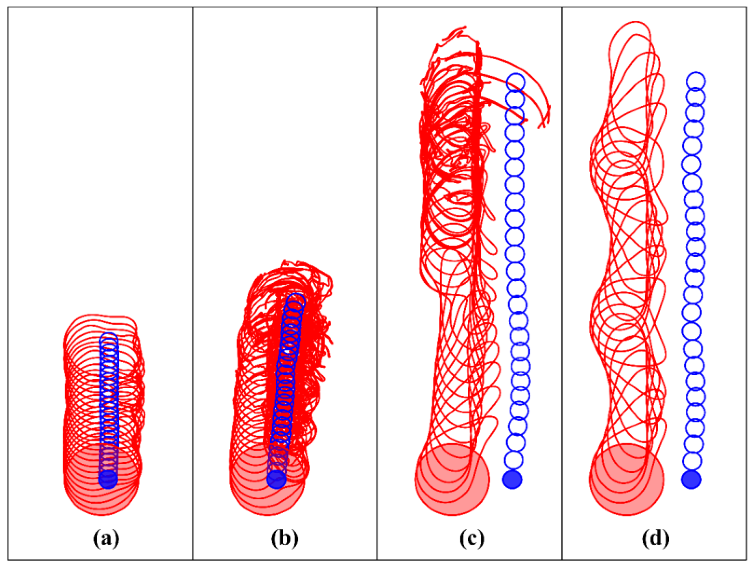
• A two-layer vortex with a vertical axis, consisting of a large-scale cyclone of the upper layer and a sufficiently large anticyclone of the middle layer, can be unstable with respect to small perturbations of the shape of the vortex patches and decompose into smaller two-layer vortex structures. In the case when the intratermocline anticyclone is of the order of Rd₁, the two-layer vortex behaves stably (Section 3.1). Note that such a vortex structure consisting of point vortices is also always stable.
• If the centers of the cyclone of the upper layer and the anticyclonic lens of the middle layer are spaced, then such a two-layer vortex can either move forward (when its total effective vorticity is zero) or rotate relative to the center of vorticity (when its total effective vorticity is nonzero). These properties are also characteristic of point vortices. For finite-core vortices, in addition, there is a certain interval of distances between their centers, in which the motion of the vortex patches is accompanied by a partial destruction of the surface cyclone and a deviation from the trajectory predicted by the theory of point vortices occurs (Section 3.2).
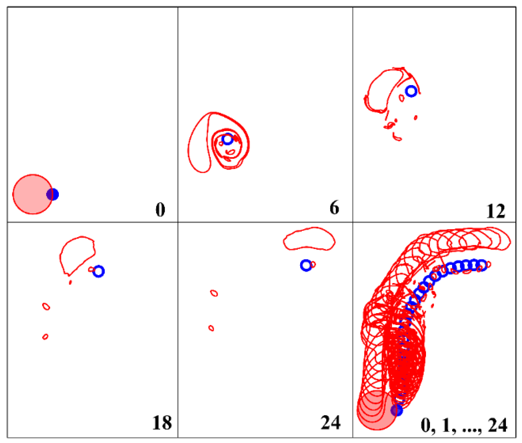
• If intrathermocline dipole is initially located below the surface vortex core, the formation of a such new type of vortex structure occurs when most of the surface cyclone core is left behind and two of its fragments pair up with the lenses and drift away. The two-layer structure including the lenses has a complex form: one part consists of two cyclonic vortex patches in the upper and middle layers, and the second part has a hetonic nature (Section 4.1).
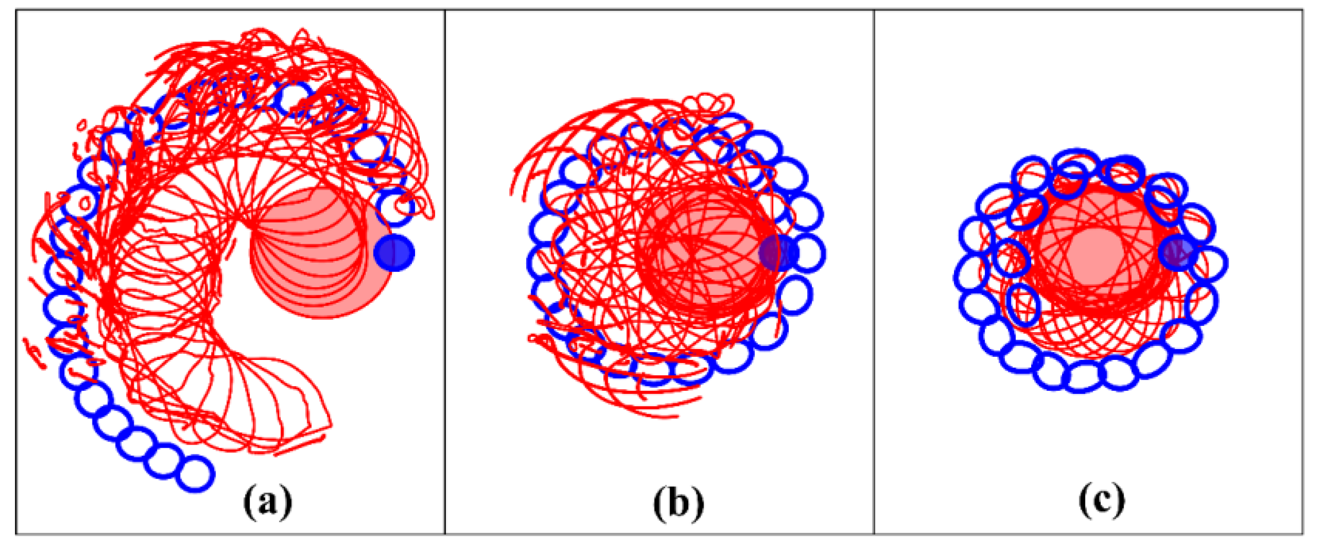
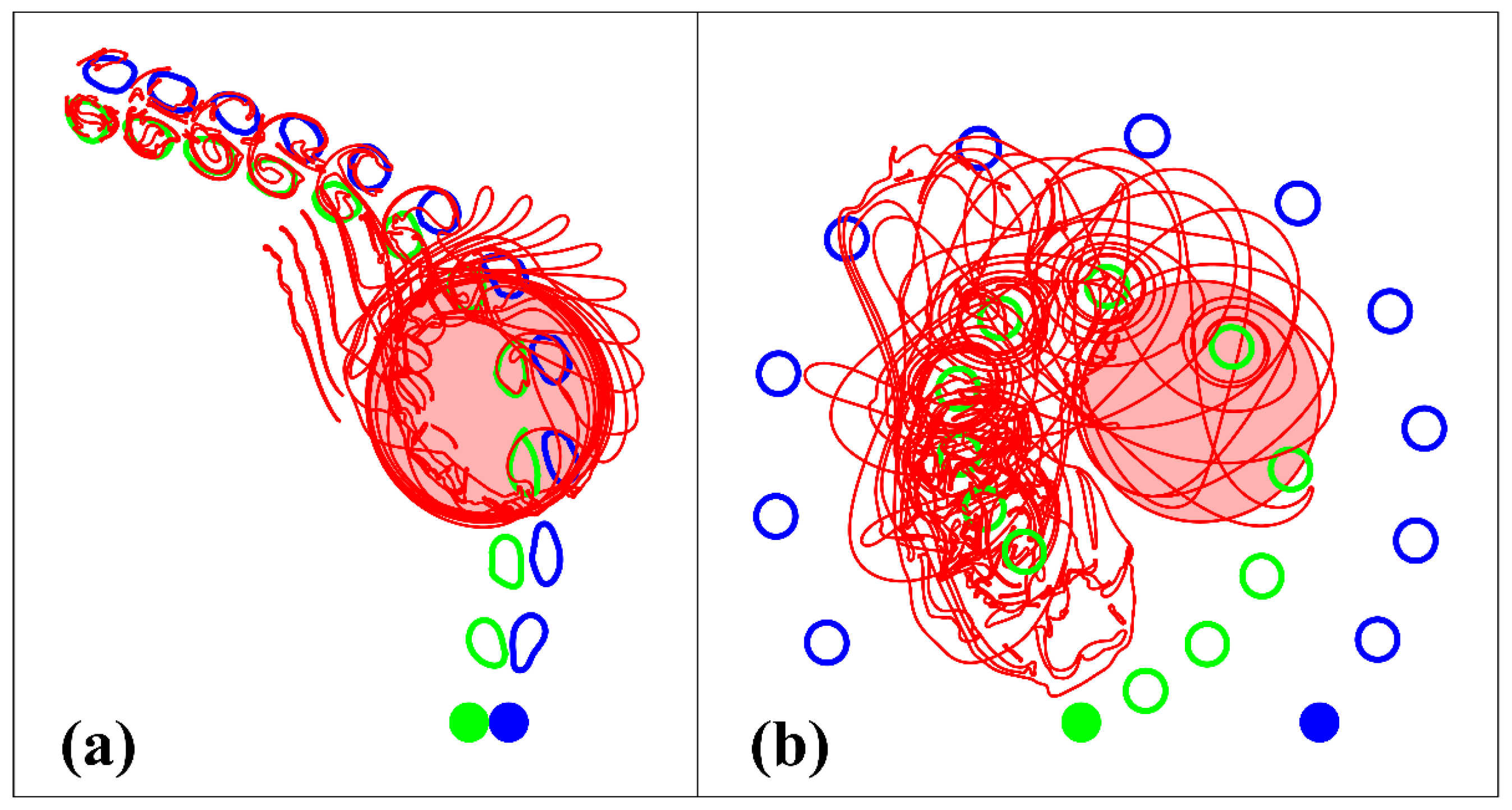
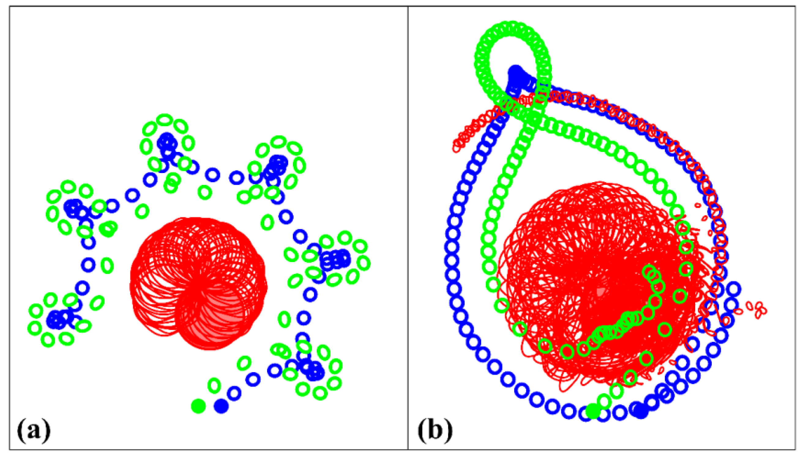
• If the intrathermocline dipole is running onto the surface vortex, then (like in the point vortex case [19]) we have two regimes: (a) the pair passes under the surface vortex, changing its direction in its vicinity and capturing part of its mass; (b) the cyclonic vortex of the intrathermocline dipole is captured by the surface cyclone, and the anticyclonic lens rotates at the periphery of the newly formed bilayer cyclonic structure; and, unlike the case of point vortices, the dipole of the middle layer cannot leave the vicinity of the surface cyclone. (Section 4.2.1).
• If an asymmetry in the distribution of potential vorticity is observed in a vortex structure incident on a surface cyclone, then it makes loop-like movements and, at the same time, rotates around the cyclone of the upper layer. It is striking that in the case of finite-core vortices (depending on the initial distance between them), states can be formed that resemble the modal structures obtained for point vortices (19) as quasi-stationary solutions (Section 4.2.2).

These findings from vortex dynamics deserve further measurements at sea, both from intensive surveys and with Lagrangian floats. It is noteworthy that since cyclonic eddies, as a rule, are weaker than anticyclonic ones at intermediate depths in the ocean [15,17], loop-shaped trajectories enveloping a surface cyclone can be most probable in nature. Further work will investigate the databases of surface drifter trajectories and of deep Argo float trajectories as an oceanographic application of this paper.

References

1. Basdevant, C.; Legras, B.; Sadourny, R.; Béland, M. A Study of Barotropic Model Flows: Intermittency, Waves and Predictability. J. Atmos. Sci. 1981, 38, 2305–2326. [Google Scholar] [CrossRef] [Green Version]
2. Benzi, R.; Patarnello, S.; Santangelo, P. Self-Similar Coherent Structures in Two-Dimensional Decaying Turbulence. J. Phys. A 1988, 21, 1221–1237. [Google Scholar] [CrossRef]
3. Melander, M.V.; Zabusky, N.J.; McWilliams, J.C. Asymmetric Vortex Merger in Two Dimensions: Which Vortex is “Victorious”? Phys. Fluids 1987, 30, 2610–2612. [Google Scholar] [CrossRef]
4. Dritschel, D.G.; Waugh, D.W. Quantification of the Inelastic Interaction of Unequal Vortices in Two-Dimensional Vortex Dynamics. Phys. Fluids A 1992, 4, 1737–1744. [Google Scholar] [CrossRef] [Green Version]
5. Yasuda, I.; Flierl, G.R. Two-Dimensional Asymmetric Vortex Merger: Contour Dynamics Experiment. J. Oceanogr. 1995, 51, 145–170. [Google Scholar] [CrossRef]
6. Trieling, R.R.; Velasco Fuentes, O.U.; van Heijst, G.J.F. Interaction of Two Unequal Corotating Vortices. Phys. Fluids 2005, 17, 087103. [Google Scholar] [CrossRef] [Green Version]
7. Brandt, L.K.; Cichocki, T.K.; Nomura, K. Asymmetric Vortex Merger: Mechanism and Criterion. Theor. Comput. Fluid Dyn. 2010, 24, 163–167. [Google Scholar] [CrossRef] [Green Version]
8. Brandt, L.K.; Nomura, K. Characterization of the Interactions of Two Unequal Co-Rotating Vortices. J. Fluid Mech. 2010, 646, 233–253. [Google Scholar] [CrossRef] [Green Version]
9. Ozugurlu, E.; Reinaud, J.N.; Dritschel, D.G. Interaction between Two Quasi-Geostrophic Vortices of Unequal Potential Vorticity. J. Fluid Mech. 2008, 597, 395–414. [Google Scholar] [CrossRef]
10. Charney, J. Geostrophic Turbulence. J. Atmos. Sci. 1971, 28, 1087–1095. [Google Scholar] [CrossRef] [Green Version]
11. McWilliams, J.C. Statistical Properties of Decaying Geostrophic Turbulence. J. Fluid Mech. 1989, 198, 199–230. [Google Scholar] [CrossRef]
12. McWilliams, J.C. The Vortices of Geostrophic Turbulence. J. Fluid Mech. 1990, 219, 387–404. [Google Scholar] [CrossRef]
13. Treguier, A.M.; Hua, B.L. Oceanic Quasi-Geostrophic Turbulence Forced by Stochastic Wind Fluctuations. J. Phys. Oceanogr. 1987, 17, 397–411. [Google Scholar] [CrossRef] [Green Version]
14. Treguier, A.M.; Hua, B.L. Influence of Bottom Topography on Stratified Quasi-Geostrophic Turbulence in the Ocean. Geophys. Astrophys. Fluid Dyn. 1988, 43, 265–305. [Google Scholar] [CrossRef]
15. Carton, X.; Daniault, N.; Alves, J.; Chérubin, L.; Ambar, I. Meddy Dynamics and Interaction with Neighboring Eddies Southwest of Portugal: Observations and Modeling. J. Geophys. Res. 2010, 115, C06017. [Google Scholar] [CrossRef] [Green Version]
16. Filyushkin, B.N.; Sokolovskiy, M.A. Modeling the Evolution of Intrathermocline Lenses in the Atlantic Ocean. J. Mar. Res. 2011, 69, 191–220. [Google Scholar] [CrossRef]
17. L’Hégaret, P.; Carton, X.; Ambar, I.; Menesguen, C.; Hua, B.L.; Chérubin, L.; Aguiar, A.; Le Cann, B.; Daniault, N.; Serra, N. Evidence of Mediterranean Water Dipole Collision in the Gulf of Cadiz. J. Geophys. Res. Oceans. 2014, 119, 5337–5359. [Google Scholar] [CrossRef] [Green Version]
18. Haynes, P.H.; McIntyre, M.E. On the Conservation and Impermeability Theorems for Potential Vorticity. J. Atmos. Sci 1990, 47, 2021–2031. [Google Scholar] [CrossRef] [Green Version]
19. Sokolovskiy, M.A.; Carton, X.J.; Filyushkin, B.N. Mathematical Modeling of Vortex Interaction Using a Three-Layer Quasigeostrophic Model. Part 1: Point-Vortex Approach. Mathematics 2020, 8, 1228. [Google Scholar] [CrossRef]
20. Sokolovskiy, M.A.; Filyushkin, B.N.; Carton, X.J. Dynamics of Intrathermocline Vortices in a Gyre Flow over a Seamount Chain. Ocean Dyn. 2013, 63, 741–760. [Google Scholar] [CrossRef]
21. Kamenkovich, V.M.; Koshlyakov, M.N.; Monin, A.S. Synoptic Eddies in the Ocean; Kamenkovich, V.M., Ed.; Kluwer Academic Publisher: Dordrecht, The Netherlands, 1986; p. 444. [Google Scholar]
22. Sokolovskiy, M.A.; Carton, X.J.; Filyushkin, B.N.; Yakovenko, I.O. Interaction between a Surface Jet and Subsurface Vortices in a Three-Layer Quasi-Geostrophic Model. Geophys. Astrophys. Fluid Dyn. 2016, 110, 201–223. [Google Scholar] [CrossRef]
23. Vallis, G.K. Atmospheric and Oceanic Fluid Dynamics. In Fundamentals and Large-Scale Circulation, 2nd ed.; Cambridge University Press: Cambridge, UK, 2017; p. 964. ISBN 9781107065505. [Google Scholar]
24. Kamenkovich, V.M.; Larichev, V.D.; Kharkov, B.V. A Numerical Barotropic Model for Analysis of Synoptic Eddies in the Open Ocean. Oceanology 1982, 21, 549–558. [Google Scholar]
25. Kozlov, V.F. The Method of Contour Dynamics in Model Problems of the Ocean Topographic Cyclogenesis. Izv. Atmos. Oceanic Phys. 1983, 19, 635–640. [Google Scholar]
26. Sokolovskiy, M.A. Modeling Triple-Layer Vortical Motions in the Ocean by the Contour Dynamics Method. Izv. Atmos. Ocean. Phys. 1991, 27, 380–388. [Google Scholar]
27. Makarov, V.G. Computational Algorithm of the Contour Dynamics Method with Changeable Topology of Domains under Study. Model. Mekh. 1991, 5, 83–95. [Google Scholar]
28. Sokolovskiy, M.A. Stability of an Axisymmetric Three-Layer Vortex. Izv. Atmos. Ocean. Phys. 1997, 33, 16–26. [Google Scholar]
29. Sokolovskiy, M.A. Stability Analysis of the Axisymmetric Three-Layered Vortex Using Contour Dynamics Method. Comput. Fluid Dyn. J. 1997, 6, 133–156. [Google Scholar]
30. Hogg, N.G.; Stommel, H.M. The heton, an Elementary Interaction Between Discrete Baroclinic Geostrophic Vortices, and its Implications Concerning Eddy Heat-Flow. Proc. R. Soc. Lond. A 1985, 397, 1–20. [Google Scholar] [CrossRef]
Figure 1. The average annual vertical density profile (solid magenta line) characteristic for the Atlantic [21] and its piecewise constant approximation (solid black line). Dashed lines indicate undisturbed interfaces between layers.
Mathematics 08 01267 g001
Figure 2. A plane section of the vortex patches which cuts the vertical axes of all three cylindrical vortices for the case when the vortices of the middle layer dipole are located under a large-scale surface vortex. The cyclone of the upper layer is colored red, and the cyclonic and anticyclonic vortices of the middle layer are green and blue, respectively. The dashed lines depict the cross-section of the deformable interface (14) between the layers under the influence of vorticity, as well as solid upper and lower surfaces.
Mathematics 08 01267 g002
Figure 3. Neutral stability curve of the two-layer axisymmetric structure composed of the synoptic surface cyclonic vortex and the anticyclonic middle-layer lens for the mode m = 2 on the plane of variables ( r 2 ; Π 2 ) with r 1 = 4 and Π 1 = 0.25 . The designations S and U correspond to stable and unstable regions. The round marker corresponds to the parameters used in the experiment shown in Figure 4.
Mathematics 08 01267 g003
Figure 4. Horizontal projections of the synchronous configurations of the vortex-patch contours of the upper (red) and middle (blue) layers at the dimensionless moments indicated on each subplot, for ( r 1 ; Π 1 ) = ( 4 ; 0.25 ) and ( r 2 ; Π 2 ) = ( 3 ; 0.60 ) , i.e., a ratio of “effective” vorticity, Ρ 1 / Ρ 2 = 0.4444 . The round marker in the region of instability in Figure 3 corresponds to this experiment.
Mathematics 08 01267 g004
Figure 5. The translational velocity V   vs .   L of the vortex structure composed of the point vortices in upper and middle layers (green line) [19] and finite-area vortex patches in the same layers (black-red line) at r 1 = 4 ; Ρ 1 = 0.6 and r 2 = 1 ; Ρ 2 = 0.6 on the distance L between vortices in the first case and their centers in the second case. The part of the curve in which the surface vortex loses its compactness and partially collapses is marked in red. Markers on the black ( L = 0.71 , L = 7.00 ) and red ( L = 1.00 , L = 6.50 ) lines correspond to the experiments presented in Figure 6.
Mathematics 08 01267 g005
Figure 6. Gallery of the superposed vortex contours in the upper layer (red lines) and middle layer (blue lines) for r 1 = 4 , r 2 = 1 and Ρ 1 = Ρ 2 = 0.6 at times t = 0 ,   1 ,   2 ,   ,   24 , and different distances between the vortices: (a) L = 0.71 ; (b) L = 1.0 ; (c) L = 6.5 ; (d) L = 7.0 (the markers in Figure 5 correspond to these values of L). Vortex patches at t = 0 are filled. The time evolution goes from bottom to top in each panel.
Mathematics 08 01267 g006
Figure 7. Motion of a two-layer heton (vertical dipolar vortex), with the same parameters r 1 , r 2 , Ρ 1 , Ρ 2 , as in Figure 6, but with L = 4 at the indicated dimensionless times.
Mathematics 08 01267 g007
Figure 8. This figure is like the last panel of Figure 8 (for which Ρ 2 = 0.6 ). Here we have (a) Ρ 2 = 0.3 , (b) Ρ 2 = 0.15 , (c) Ρ 2 = 0.075 .
Mathematics 08 01267 g008
Figure 9. Interaction of a surface cyclonic vortex with P 1 = 0.6 and the pair of vortex patches located in the middle layer with r 2 1 = r 2 2 = 1 , Ρ 2 1 = Ρ 2 2 = 0.01875 at L = 1 . The contour of the cyclonic/anticyclonic vortex in the middle layer is in green/blue: (a) r 1 = 4 , (b) r 1 = 6 .
Mathematics 08 01267 g009
Figure 10. An intrathermocline dipole, approaching the surface cyclone at P 1 = 0.6 , r 1 = 6 , r 2 1 = r 2 2 = 1 , Ρ 2 1 = Ρ 2 2 = 0.3 , y 2 1 = y 2 2 = 16 at t = 1 ,   2 ,   ,   12 : (a) L = 1 , (b) L = 6 .
Mathematics 08 01267 g010
Figure 11. Sets of superimposed vortex patches contour at r1=6, r 2 1 = r 2 2 = 1 , Ρ 2 1 / Ρ 2 2 = 1 / 2 , Ρ 2 1 / Ρ 1 1 = 1 / 2 , y 2 1 = y 2 2 = 16 , and (a) L = 2 , (b) L = 4 .
Mathematics 08 01267 g011