Static and Dynamic Properties of a Few Spin 1/2 Interacting Fermions Trapped in a Harmonic Potential

Abstract

We provide a detailed study of the properties of a few interacting spin $1/2$ fermions trapped in a one-dimensional harmonic oscillator potential. The interaction is assumed to be well represented by a contact delta potential. Numerical results obtained by means of direct diagonalization techniques are combined with analytical expressions for both the non-interacting and strongly interacting regime. The $N=2$ case is used to benchmark our numerical techniques with the known exact solution of the problem. After a detailed description of the numerical methods, in a tutorial-like manner, we present the static properties of the system for $N=2,3,4$ and 5 particles, e.g., low-energy spectrum, one-body density matrix, ground-state densities. Then, we consider dynamical properties of the system exploring first the excitation of the breathing mode, using the dynamical structure function and corresponding sum-rules, and then a sudden quench of the interaction strength.

1. Introduction

The theoretical study of one-dimensional systems has always attracted a lot of attention. Very early in the development of quantum mechanics it was recognized that reducing the dimensionality of the systems enhances the quantum effects and gives origin to a plethora of interesting phenomena, see for instance Ref. [1] and references therein. After the pioneering work of Tonks, who investigated the equation of state of hard-rods, hard disks and hard-spheres in one, two and three dimensions, respectively [2], Girardeau established the map between impenetrable bosons and free fermions in one dimension [3]. However, it took a long time until the experimental realization of these systems became a reality [4,5,6]. This experimental breakthrough took place in the context of the ultracold gases that have developed a frenetic experimental and theoretical activity during the last years achieving unbelievable possibilities to control the geometry, the interactions and the number of particles for many types of setups [7,8,9,10]. More recently, the groundbreaking experiments of Jochim’s group in Heildelberg, have opened new theoretical challenges to study one-dimensional fermionic systems. They have been able to precisely control the number of atoms and the strength of the interactions [11]. These experiments have provided deep insight in the expected phenomena of fermionization of two distinguishable fermions [12], i.e., with different third spin component. In addition, they have been able to change the number of particles, going from few to many particles, and being able to study the appearance of correlations in the many-body wave function. In fact, by adding particles to the system one by one, it was shown how the many-body correlated system is built [13]. These experiments used ${}^6$Li atoms and took advantage of the Feshbach resonance mechanism to modulate the interactomic interaction [14]. Consequently, many theoretical problems have been addressed and few- and many-body techniques for ab-initio descriptions used in other fields have been specially tailored for these many-body one-dimensional systems. The impurity problem, the presence of pairing phenomena in few-fermion systems [15], the behaviour of two fermions in a double-well potential [16], the realization of an antiferromagnetic spin chain of few cold atoms [17], all belong to the long list of theoretical challenges that the experimental advances are offering to theoreticians. They are looking at those systems as a very versatile laboratory where they apply ab-initio techniques, without the complexity of the inter-particle interactions that appear in other fields, as for instance in nuclear physics [18,19]. Reciprocally, the technological control is such that ultracold atomic systems can also be used as quantum simulators to solve very intricate condensed-matter problems [9]. Although we will not pay attention to them in this paper it is worth mentioning that trapping and control of the interactions have been extended also to mixtures of different nature and statistics: mixtures of bosons, and bosons and fermions [20,21,22,23,24,25].

In this work, we consider a system of a few spin-$1/2$ fermions trapped in a one-dimensional harmonic trap. The interaction between the fermions is modeled by a contact potential. In the literature there are some studies under similar conditions [25,26,27,28,29,30,31,32,33]. We pay attention both to the ground state and energy spectrum of the system and also to the dynamical properties of few-fermion systems depending on the interaction strength and the number of particles [34,35].

The structure of this work is the following. In Section 2, we present the theoretical description of the fermionic system, composed by a fixed number of atoms with spin up and down. In particular, we write down the full Hamiltonian both in first and second quantized form. Some limiting scenarios are considered, e.g., both zero and strong interaction. In Section 3, we describe the numerical tools used to study the ground state and low-excited states of the fermionic mixture. The main method employed is direct diagonalization of the Hamiltonian matrix in a truncated Hilbert space. In Section 4, we study the ground state of the system for different number of fermions and polarizations. In Section 5 we turn our attention to the lower part of the spectrum, computing the spectra for the same few-fermion systems considered. In Section 6, we compute the response of the system to two different external perturbations. Finally in Section 7 we provide the main conclusions of our work.

2. Theoretical Approach

In this section we introduce the theoretical tools to describe a system composed of a few fermions trapped in a one dimensional harmonic oscillator potential. The goal is to provide a self-contained explanation of the methods employed, detailing the numerical subtleties encountered.

2.1. The Hamiltonian of the System

The Hamiltonian of the system can be split in two parts, the non-interacting single-particle part, which describes particles trapped in a harmonic oscillator potential, and the two-body interaction part, which describes the interactions between the fermions. The Hamiltonian, in first quantized form, can be written as [33,35]

$$H=H_{\mathrm{ho}}+\sum _{i<j}^N{V}_{\mathrm{int}}(x_i-x_j),$$

(1)

where $H_{\mathrm{ho}}={\sum }_i{h}_{\mathrm{ho}}\left(i\right)$ is the sum of single-particle harmonic oscillator Hamiltonians. The Hamiltonian, $h_{\mathrm{ho}}$, is a one-body operator, which includes the kinetic- and the harmonic-potential energy,

$$h_{\mathrm{ho}}=-\frac{{\hslash }^2}{2m}\frac{{\partial }^2}{\partial x^2}+\frac{1}{2}m{\omega }^2{x}^2,$$

(2)

where m is the particle mass and $\omega$ is the harmonic oscillator frequency. The eigenvalues of this Hamiltonian are well known,

$$e_n=\left(n+\frac{1}{2}\right)\hslash \omega n=0,1,2,\dots ,$$

(3)

and the corresponding eigenfunctions are written as,

$${\Phi }_n\left(x\right)=\frac{1}{\sqrt{2^{n}n!}}{\left(\frac{m\omega }{\pi \hslash }\right)}^{1/4}{e}^{-\frac{m\omega x^2}{2\hslash }}{H}_n\left(\sqrt{\frac{m\omega }{\hslash }}x\right),$$

(4)

where $H_n\left(x\right)$ is the n-th Hermite polynomial. These single-particle wave functions will be used to build the many-body basis. All these wave functions have a similar structure: a Gaussian function multiplied by a Hermite polynomial with a normalization factor, that depends on n.

We consider identical spin $1/2$ fermions, i.e., with two possible spin states: $|1/2,m\rangle$, $m=1/2,-1/2$, where m is the spin projection on the z-axis. Sometimes, these two spin states are denoted by: |↑〉 and |↓〉, respectively. The fermions are assumed to interact via a contact spin-independent delta potential [36]. Therefore two fermions interact only if they are at the same position. However, the many-body wave function of a system of identical fermions should be antisymmetric, preventing two fermions with the same spin from being at the same position. Therefore, fermions with the same spin projection do not interact, and thus the contact interaction is only acting between fermions with different spin projection.

In any case, the total wave function including the spin degree of freedom should be antisymmetric. This requirement allows the system to have two particles with different spin projection in the same position.

The interaction term of Equation (1) is a contact interaction, which is expressed as [36]

$$V_{\mathrm{int}}(x_i-x_j)=g\delta (x_i-x_j),$$

(5)

where g characterizes the strength of the interaction and $\delta$ is a Dirac delta function.

Taking into account the identity [34]

$$\sum _{i=1}^N{x}_i^2=N{X}^2+\frac{1}{N}\sum _{i<j}{(x_i-x_j)}^2,$$

(6)

where $X=\frac{1}{N}{\sum }_i{x}_i$ is the center of mass coordinate, the Hamiltonian can be split in two pieces,

$$H=H_{\mathrm{CM}}+H_{\mathrm{r}},$$

(7)

where $H_{CM}$ in harmonic oscillator units reads:

$$H_{CM}=-\frac{1}{2N}\frac{d^2}{d{X}^2}+\frac{N}{2}{X}^2,$$

(8)

and governs the center-of-mass motion. $H_r$ affects only the relative coordinates and is translationally invariant.

One way to create a one-dimensional trap is using a cigar-shaped trapping potential, with the transverse trap frequency ${\omega }_{\perp }$ (in the radial direction) much larger than the trap frequency $\omega$ in the axial direction. In this situation, the coupling constant g is related to the one-dimensional scattering length ($a_{1\mathrm{d}}$) as [36,37],

$$g=-\frac{{\hslash }^2}{m{a}_{1\mathrm{d}}}.$$

(9)

From the relation between the one-dimensional scattering length and the three-dimensional scattering length [38], we can write the coupling constant as

$$g=\frac{2{\hslash }^2{a}_{3\mathrm{d}}}{m{a}_{\perp }^2}\frac{1}{1-|\xi (1/2)|a_{3\mathrm{d}}/\left(\sqrt{2}{a}_{\perp }\right)},$$

(10)

with $a_{\perp }=\sqrt{\hslash /m{\omega }_{\perp }}$ and $\xi$ is the Riemann zeta function.

In a trap under these conditions, the system can be treated as a one-dimensional system. As the trapping in the transverse dimension is very strong, all particles occupy the lowest state of the transverse harmonic oscillator and the physics takes place in the longitudinal direction [38].

For convenience we use the harmonic oscillator units, in which the energy is measured in $\hslash \omega$ units, the length in units of $\sqrt{\hslash /m\omega }$ and the coupling constant g is expressed in units of $\sqrt{\omega {\hslash }^3/m}$. From this moment on, all magnitudes will be expressed in these units.

2.2. Non-Interacting and Infinite Interaction Limits

In general, it is not possible to solve analytically the Schrödinger equation for an arbitrary value of the interaction strength. However, there are two limits, i.e., the non-interacting and the infinite interaction cases, in which one has explicit analytical solutions [39,40].

For these two limits, one can easily determine the energy and the density profile of the ground state of the system, and explicitly write the wave function.

2.2.1. Non-Interacting Case: Fermi Gas

In the non-interacting case, the system is in a state called Fermi gas. In these conditions, the behavior of the system is given by the single-particle states of the harmonic oscillator with the restriction of the Pauli principle that does not allow two fermions with the same spin projection in the same harmonic oscillator state. More specifically, in the ground state of a system with $N_d$ particles of spin down and $N_u$ particles of spin up, the particles occupy the lowest single-particle energy states, $N_d$ and $N_u$, respectively. Therefore, the energy of the ground state is

$$E_{\mathrm{gs}}(g=0)=\sum _{n=0}^{N_d-1}\left(n+\frac{1}{2}\right)+\sum _{n=0}^{N_u-1}\left(n+\frac{1}{2}\right)=\frac{N_d^2+N_u^2}{2}.$$

(11)

Actually the wave function of the system is given by a Slater determinant built with the lowest $N_u$ and $N_d$ single-particle wave functions with spin up and down, respectively. The total third component of the spin of this wave function is $M=\frac{N_u-N_d}{2}$ and the total spin is the minimum S compatible with M, $S=M$ [41]. For a non-polarized system, $N_u=N_d$, then $M=0$ and $S=0$.

The density profile associated to this wave function is the sum of the probabilities of finding a particle in each occupied state in the position x,

$$\rho \left(x\right)=\sum _{n=0}^{N_d-1}|{\Phi }_n\left(x\right){|}^2+\sum _{n=0}^{N_u-1}{|{\Phi }_n\left(x\right)|}^2,$$

(12)

where ${\Phi }_n\left(x\right)$ are the 1D harmonic oscillator wave functions, Equation (4). The density profile is normalized to the number of particles.

2.2.2. Infinite Interaction Case

In the infinite interaction limit, the system experiences a phenomenon reminiscent of the fermionization process in Bose systems [2,3]. The ground state of the Hamiltonian in the infinite interaction limit for a fully- polarized state is a Slater determinant of the N first harmonic oscillator states, ${\Psi }_A$. For a non fully-polarized case the ground state many-fold is degenerate, with degeneration $D=N!/(N_u!N_d!)$ [33] and total third spin component $M=(N_u-N_d)/2$. The states can be written as [40],

$$\Psi =\sum _{k=1}^D{a}_k\theta (x_{P_k\left(1\right)},\dots ,x_{P_k\left(N\right)}){\Psi }_A(x_1,\dots ,x_N),$$

(13)

where $\theta (x_1,\dots ,x_N)=1$ when $x_1<x_2<\dots <x_N$ and zero otherwise, $P_k$ are the D permutations of the N components and the $a_k$ are the coefficients for each permutation. In this expression we have fixed the first $N_u$ particles to be spin projection up and the remaining $N_d$ particles to have spin projection down. Their energy depends only on the single-particle states present in ${\Psi }_A$,

$$E_{\mathrm{gs}}(g\to \infty )=\sum _{n=0}^{N-1}\left(n+\frac{1}{2}\right)=\frac{{(N_d+N_u)}^2}{2}.$$

(14)

The density profile associated to these wave functions is the sum of the probabilities of finding a particle in each occupied state in the position x [42],

$$\rho \left(x\right)=\sum _{n=0}^{N-1}{|{\Phi }_n\left(x\right)|}^2,$$

(15)

where ${\Phi }_n\left(x\right)$ are the 1D harmonic-oscillator wave functions, Equation (4).

2.3. Second Quantization

When working with several particles, it is useful to use the second-quantization formalism. One of the main ingredients of this formalism is the many-body Fock space. In order to define the Fock space, we need to have a single-particle basis, such as the harmonic oscillator states. The basis of the Fock space is constructed by indicating how many particles occupy each single-particle state. In addition, the antisymmetry rules are implemented by the anticommutation rules fulfilled by the creation and annihilation operators [43].

A particular state is the vacuum state denoted by |0〉. This vector represents a state without particles, i.e., all its occupation numbers are zero. This state has norm equal to 1.

2.3.1. Creation and Annihilation Operators

The main tool in second quantization are the creation $\left(a_i^{†}\right)$ and annihilation $\left(a_i\right)$ operators, which act on the Fock space. Any observable, which is represented by an operator, can be expressed in terms of them [43]. The action of a creation operator on the vacuum state, denoted as $a_i^{†}|0\rangle$, creates a particle in the state i. In general, acting with a creation operator on a Fock space vector, creates a particle in the i-th state, whenever possible. Or in other words, it increases the occupation number of this single-particle state by one. On the other hand, the action of an annihilation operator ($a_i$) on a state destroys a particle in the i-th state, whenever possible. In other words, it decreases the occupation number of the state by one.

In addition, a Fock space vector with N particles can be created by the action of N creation operators on the vacuum space, as follows,

$$|n_1,n_2,n_3,\dots ,n_m\rangle ={\left(a_1^{†}\right)}^{n_1}{\left(a_2^{†}\right)}^{n_2}{\left(a_3^{†}\right)}^{n_3}\dots {\left(a_m^{†}\right)}^{n_m}|0\rangle$$

(16)

with $N={\sum }_i{n}_i$.

In the case of fermions, to satisfy the Pauli principle, i.e., the antisymmetry of the wave function, the creation and annihilation operators should fulfill the following anti-commutation relations

$$\begin{array}{cc}\hfill & \left\{a_i^{†},a_j\right\}={\delta }_{ij}\hfill \\ \hfill & \left\{a_i^{†},a_j^{†}\right\}=\left\{a_i,a_j\right\}=0.\hfill \end{array}$$

(17)

Therefore the occupation number of the Fock basis can take the values $n_i=0$ or $n_i=1$. Finally, the action of the creation and annihilation operators can be written as

$$\begin{array}{cc}\hfill & a_i^{†}|n_1,n_2,\dots n_{i-1},n_i,\dots \rangle ={(-1)}^{N_i}(1-n_i)|n_1,n_2,\dots n_{i-1},(1-n_i),\dots \rangle \hfill \\ \hfill & a_i|n_1,n_2,\dots n_{i-1},n_i,\dots \rangle ={(-1)}^{N_i}{n}_i|n_1,n_2,\dots n_{i-1},(1-n_i),\dots \rangle ,\hfill \end{array}$$

(18)

where $N_i$ is the number of occupied states with index lower than i,

$$N_i=\sum _{k=1}^{i-1}{n}_k.$$

(19)

The phase ${(-1)}^{N_i}$ is due to the anti-commutation relations. Notice that the factor in front of the state becomes zero if one tries to put two particles in the same single-particle state or one tries to annihilate a particle in a single-particle state which is not occupied.

2.3.2. Fock Space

The harmonic oscillator eigenfunctions are used to build the many-body basis of the Fock space. In addition, the spin degrees of freedom are also incorporated to the single particle wave functions which are defined as: ${\phi }_{n,m}(x,s)={\Phi }_n\left(x\right){\chi }_m\left(s\right)$, where ${\Phi }_n\left(x\right)$ is the harmonic oscillator wave function of the level n and ${\chi }_m$ is the spin wave function, where $m=\uparrow (\downarrow )$ is the spin projection.

With these single-particle states, we build the many-body basis of the Fock space:

$$|n_{0\downarrow },n_{0\uparrow },n_{1\downarrow },n_{1\uparrow },\dots \rangle ,$$

(20)

where $n_{i,m}$ indicates the number of particles in the ${\phi }_{i,m}$ single-particle state.

2.3.3. Operators in Second Quantization

In second quantization, operators can be expressed in terms of creation and annihilation operators. A general one-body operator $\widehat{\mathcal{O}}$ is expressed as

$$\widehat{\mathcal{O}}=\sum _{i,j}\langle i|\widehat{O}|j\rangle a_i^{†}{a}_j,$$

(21)

where |i〉 and |j〉 are single-particle states, $\langle i|\widehat{O}|j\rangle =\int {\phi }_i^{*}\left(x\right)O\left(x\right){\phi }_j\left(x\right)dx$ is the one-body matrix element and ${\phi }_i\left(x\right)$ are the single-particle wave functions used to build the Fock space. Notice that the sub-index i stands for all the quantum numbers necessary to specify the single-particle state.

A general two-body operator $\widehat{\mathcal{V}}$ is expressed as

$$\widehat{\mathcal{V}}=\frac{1}{2}\sum _{i,j,k,l}\langle i,j|\widehat{V}|k,l\rangle a_i^{†}{a}_j^{†}{a}_l{a}_k=\frac{1}{2}\sum _{i,j,k,l}{v}_{ij,kl}{a}_i^{†}{a}_j^{†}{a}_l{a}_k,$$

(22)

where $v_{ij,kl}$ is the two-body matrix element defined as

$$v_{ij,kl}=\int {\phi }_i^{*}\left(x_1\right){\phi }_j^{*}\left(x_2\right)\mathcal{V}(x_1,x_2){\phi }_k\left(x_1\right){\phi }_l\left(x_2\right)d{x}_{1}d{x}_2.$$

(23)

2.3.4. The Hamiltonian in Second Quantization

As already mentioned, the Hamiltonian describing the harmonic oscillator is a one-body operator. On the other hand, the interaction term Equation (1) is a two-body operator. In our case, choosing the harmonic-oscillator eigenfunctions as the single-particle basis, the Hamiltonian part corresponding to the harmonic oscillator is diagonal, with eigenvalues ${ϵ}_i=i+1/2$. Therefore in second quantization it reads,

$${\widehat{h}}_{\mathrm{ho}}=\sum _i{ϵ}_i{a}_i^{†}{a}_i=\sum _i{ϵ}_i{\widehat{n}}_i,$$

(24)

where ${\widehat{n}}_i=a_i^{†}{a}_i$ is the number operator associated to the single-particle state |i〉. For the interaction term, the two-body matrix elements are expressed as

$$\begin{array}{cc}\hfill v_{ij,kl}=& \int d{x}_{1}d{x}_2{\phi }_{i,m_i}^{*}(x_1,s_1){\phi }_{j,m_j}^{*}(x_2,s_2)g\delta (x_1-x_2){\phi }_{k,m_k}(x_1,s_k){\phi }_{l,m_l}(x_2,s_l)\hfill \\ \hfill =& g\int dx{\Phi }_i^{*}\left(x\right){\Phi }_j^{*}\left(x\right){\Phi }_k\left(x\right){\Phi }_l\left(x\right)\langle {\chi }_{m_i}{\chi }_{m_j}|{\chi }_{m_k}{\chi }_{m_l}\rangle \hfill \\ \hfill =& g{\delta }_{m_i,m_k}{\delta }_{m_j,m_l}\int dx{\Phi }_i^{*}\left(x\right){\Phi }_j^{*}\left(x\right){\Phi }_k\left(x\right){\Phi }_l\left(x\right).\hfill \end{array}$$

(25)

Notice that the interaction does not affect the spin of the particles, and we have used the orthogonality of the spin functions: $\langle {\chi }_{m_i}{\chi }_{m_j}|{\chi }_{m_k}{\chi }_{m_l}\rangle ={\delta }_{m_i,m_k}{\delta }_{m_j,m_l}$. The calculation of the integral can be found in Section 3.2. Notice that the indices labeling the single-particle states run over the harmonic oscillator wave functions and the spin projections. Finally, the Hamiltonian reads

$$H=\sum _i{\widehat{n}}_i{ϵ}_i+\frac{1}{2}\sum _{ijkl}{v}_{ij,kl}{a}_i^{†}{a}_j^{†}{a}_l{a}_k.$$

(26)

3. Numerical Methods

In this chapter we describe the method named direct diagonalization to find an approximate solution of the many-body Schrödinger equation. The technical aspects on how to construct the matrix Hamiltonian, to choose a suitable many-body basis of the Fock space, and how to calculate the two-body matrix elements are discussed in detail. Finally, we use the two-particle system, that has an analytical solution [44], as a benchmark of our numerical procedure.

3.1. Direct Diagonalization

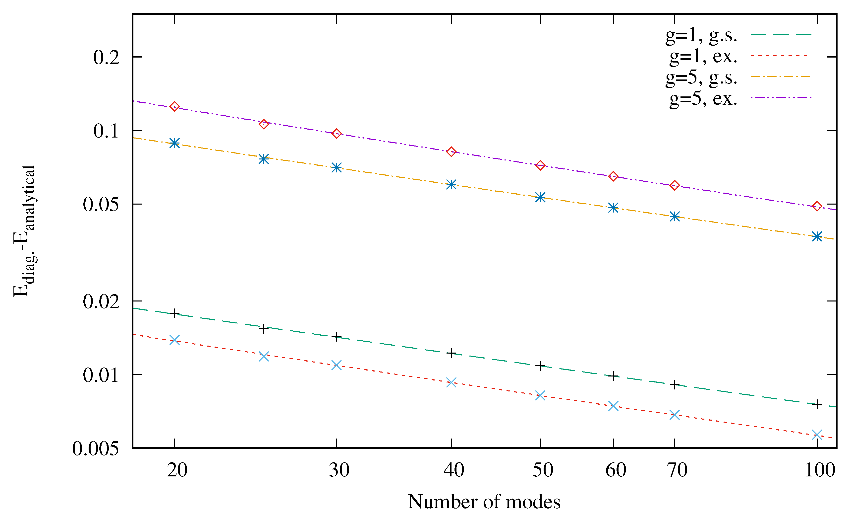
In order to study the ground state and the low-excited states of a system, one has to solve the many-body Schrödinger equation. With this objective, we use a direct diagonalization in a truncated basis space. This method needs to built the Hamiltonian matrix in an appropriate subspace and diagonalize it. In order to obtain accurate results we need to use a large basis, generating large matrices. To diagonalize these large matrices, we use a Lanczos method implemented by the ARPACK package [45]. This method allows us to diagonalize large matrices, and obtain the lowest eigenvalues with high accuracy. Hence, the direct diagonalization method allows one to obtain the ground state and the low-energy spectrum and the corresponding states. Other strategies can also provide the lowest part of the spectrum, such as the Multi Configuration Time Dependent Hartree (MCTDH) [46], used in Ref. [27] for few-fermion systems. In contrast, methods such as Monte Carlo [47], or Density Matrix Renormalization Group (DMRG) [48], are usually used to compute ground state properties.

We consider systems with 2 to 5 fermions. These particles have spin 1/2, therefore for N particles we can have $N+1$ possible total spin projections. As the Hamiltonian commutes with the total third spin component, the Hamiltonian is built in boxes with well defined M. Thus, it is possible to treat each total spin projection independently [33]. The simplest case is when all fermions have spin up, then $M=N/2$, and the wave function factorizes in an antisymmetric spatial wave function and a symmetric spin wave function $\chi (S=N/2,M=N/2)$ for N particles. The antisymmetric spatial wave function is a Slater determinant built with the lowest single-particle states. The antisymmetry of the wave function prevents two particles from being in the same position and the particles in this wave function do not feel the contact interaction. Therefore, its energy is independent of the interaction strength.

The other trivial cases are the negative M values because due to the spin symmetry of the Hamiltonian, the properties of the states do not depend on the sign of the spin projection. The diagonalization of a Hamiltonian box with a given M would provide the same eigenvalues that the box with total spin projection $-M$. Therefore we concentrate in the study of cases with $M\ge 0$.

Basis Truncation

To obtain the exact results, when using a diagonalization method, we would need to use a complete basis. However this is not possible because of the infinite dimension of the Hilbert space. Therefore we are forced to diagonalize the Hamiltonian in a finite subspace. Usually, this procedure does not provide the exact eigenvalue. However, the lowest-energy obtained by diagonalization is still an upper-bound to the ground-state energy. Note this is in contrast to exact diagonalization problems in small and discrete spaces, modelling finite optical lattices [49], where the method provides the exact values within machine precision.

A common way to construct a finite many-body basis is considering a finite number of single-particle states, usually, those with the lowest energy [49]. In our case, we diagonalize the Hamiltonian in a subspace with well-defined total third spin component. We start considering the lowest $N_M$ single-particle states and take into account an energy constraint in the construction of the many-body basis: the energy of the many-body basis states, which is given by the sum of the single-particle energies, should be smaller or equal than a fixed energy $E_{\max }$, this procedure is described in [50,51].

This maximum energy depends on the number of particles and spin configuration. Notice that we consider always $M>0$ therefore, $N_u>N_d$. The maximum energy, $E_{\max }$, corresponds to the energy of a non-interacting many-body state built as follows: one spin-up particle in the maximum single-particle energy state and the remaining ($N_u-1$) spin-up particles in the lowest $N_u-1$ single-particle states. On the other hand the $N_d$ spin-down particles are located in the lowest $N_d$ single-particle states. Therefore, the maximum energy considered in the construction of the many-body basis is

$$E_{\max }={\sum }_{n=0}^{N_d-1}\left(n+\frac{1}{2}\right)+{\sum }_{n=0}^{N_u-2}\left(n+\frac{1}{2}\right)+\left(\left(N_M-1\right)+\frac{1}{2}\right)=\frac{{\left(N_d\right)}^2+{\left(N_u-1\right)}^2}{2}+\left(N_M-\frac{1}{2}\right),$$

(27)

where $N_M$ is the number of single-particle states used.

One can see in

Table 1. Number of single-particle states used in the construction of the many-body basis states in the second column. The number of many-body basis states, with and without energy restriction, are shown in the third and fourth columns, respectively.

	Number of Single-Particle States	Number of Many-Body Basis States
		with Energy Restriction	without Restriction
2 particles, M = 0	100	5050	10,000
3 particles, M = 1/2	50	10,725	61,250
4 particles, M = 0	40	30,800	608,400
4 particles, M = 1	40	19,530	395,200
5 particles, M = 1/2	30	22,923	1,766,100
5 particles, M = 3/2	30	11,349	822,150

that the dimension of the many-body basis is strongly reduced if the energy restriction discussed above is taken into account. Nevertheless, the reduction of the size of the space considered does not affect the quality of the results in the low-energy regime of the spectrum that we are exploring in this paper. The dimension of the many-body basis in the case without energy restriction is

$$\frac{\left(N_M\right)!}{(N_M-N_u)!N_u!}\frac{\left(N_M\right)!}{(N_M-N_d)!N_d!},$$

(28)

which grows very rapidly.

In the table we have omitted the configurations with a maximum value of M, which correspond to trivial cases, with only one configuration built as the product of a symmetric spin function, with all spins parallel and an antisymmetric spatial function built with the lowest single-particle energy wave functions. As has been said previously, these configurations do not feel the effects of a contact interaction.

3.2. The Two-Body Matrix Elements of the Interaction

The evaluation of the two-body interaction on the many-body Fock basis, requires the calculation of two-body interaction matrix elements, Equation (25). These matrix elements contain an integral with four wave functions,

$$\begin{array}{cc}\hfill v_{ij,kl}=& g{\delta }_{m_i,m_k}{\delta }_{m_j,m_l}\int dx{\Phi }_i^{*}\left(x\right){\Phi }_j^{*}\left(x\right){\Phi }_k\left(x\right){\Phi }_l\left(x\right)\hfill \\ \hfill =& g{\delta }_{m_i,m_k}{\delta }_{m_j,m_l}{I}_{ijkl}.\hfill \end{array}$$

(29)

The integral, that we label as $I_{abcd}$ can be solved analytically, because the wave functions are the harmonic oscillator wave functions Equation (4),

$$\begin{array}{cc}\hfill I_{abcd}& ={\int }_{-\infty }^{\infty }{\Phi }_a\left(x\right){\Phi }_b\left(x\right){\Phi }_c\left(x\right){\Phi }_d\left(x\right)dx\hfill \\ \hfill & =\frac{1}{\pi \sqrt{2^{a+b+c+d}a!b!c!d!}}{\int }_{\infty }^{\infty }{e}^{-2x^2}{H}_a\left(x\right)H_b\left(x\right)H_c\left(x\right)H_d\left(x\right)dx.\hfill \end{array}$$

(30)

Let us consider,

$$I_{abcd}^{{}^{\prime }}={\int }_{-\infty }^{\infty }{e}^{-2x^2}{H}_a\left(x\right)H_b\left(x\right)H_c\left(x\right)H_d\left(x\right)dx.$$

(31)

We notice that this integral has to be zero if ($a+b+c+d$) is an odd number. This is because the ${\Phi }_i$ wave functions have well-defined parity. Therefore if the multiplication of the four functions is odd, the integral value is zero. This is why we only calculate the integrals with ($a+b+c+d$) even.

Using the properties [52]

$$\begin{array}{cc}\hfill & {\int }_{-\infty }^{\infty }{e}^{-2x^2}{H}_a\left(x\right)H_b\left(x\right)H_c\left(x\right)=\hfill \\ \hfill & =\frac{2^{(a+b+c-1)/2}}{\pi }\Gamma \left(\frac{a+b-c+1}{2}\right)\Gamma \left(\frac{a-b+c+1}{2}\right)\Gamma \left(\frac{-a+b+c+1}{2}\right),\hfill \end{array}$$

(32)

and

$$H_m\left(x\right)H_n\left(x\right)=2^{n}n!\sum _{r=0}^n\frac{m!}{(n-r)!(m-n+r)!}\frac{H_{m-n+2r}\left(x\right)}{2^{r}r!},n\le m.$$

(33)

We can express the integral $I_{abcd}^{{}^{\prime }}$ as

$$\begin{array}{cc}\hfill I_{abcd}^{{}^{\prime }}=& 2^{d}d!\sum _{r=0}^d\frac{c!}{(d-r)!(c-d+r)!}\frac{1}{2^{r}r!}\frac{2^{(a+b+c-d+2r-1)/2}}{\pi }\hfill \\ \hfill & \times \Gamma \left(\frac{a+b-c+d+1}{2}-r\right)\Gamma \left(\frac{a-b+c-d+1}{2}+r\right)\hfill \\ \hfill & \times \Gamma \left(\frac{-a+b+c-d+1}{2}+r\right).\hfill \end{array}$$

(34)

Notice that the arguments of the gamma functions ($\Gamma$) are half-integers. Because ($a+b+c+d$) is even, then when changing any sign, the result will remain even, and the gamma functions read,

$$\left.\begin{array}{cc}\hfill & \Gamma \left(n+\frac{1}{2}\right)=\sqrt{\pi }\frac{\left(2n\right)!}{2^{n}n!}\hfill \\ \hfill & \Gamma \left(\frac{1}{2}-n\right)=\sqrt{\pi }\frac{{(-4)}^{n}n!}{\left(2n\right)!}\hfill \end{array}\right\},n\ge 0.$$

(35)

Finally, the integral $I_{abcd}$ can be expressed as

$$\begin{array}{cc}\hfill I_{abcd}=& \frac{1}{{\pi }^2\sqrt{2}}\sqrt{\frac{c!d!}{a!b!}}\sum _{r=0}^d\frac{1}{r!(d-r)!(c-d+r)!}\Gamma \left(\frac{a+b-c+d+1}{2}-r\right)\hfill \\ \hfill & \times \Gamma \left(\frac{a-b+c-d+1}{2}+r\right)\Gamma \left(\frac{-a+b+c-d+1}{2}+r\right).\hfill \end{array}$$

(36)

The presence of factorials in the expressions of the harmonic oscillator wave functions can cause fake overflows in the calculation. One possible solution to this problem is by taking logarithms of the expressions to be evaluated. As shown before, a suitable way to write the integrals entering in the two-body matrix elements is

$$\begin{array}{cc}\hfill I_{abcd}=& \sum _{r=0}^d\frac{1}{{\pi }^2\sqrt{2}}\sqrt{\frac{c!d!}{a!b!}}\frac{1}{r!(d-r)!(c-d+r)!}\Gamma \left(\frac{a+b-c+d+1}{2}-r\right)\hfill \\ \hfill & \times \Gamma \left(\frac{a-b+c-d+1}{2}+r\right)\Gamma \left(\frac{-a+b+c-d+1}{2}+r\right).\hfill \end{array}$$

(37)

This expression can be written as $I={\sum }_r^{d}f(a,b,c,d,r)$, where f is a well-behaved function. Furthermore, we can write this result as

$$I_{abcd}=\sum _{r=0}^{d}exp\{log\left[f\right(a,b,c,d,r\left)\right]\},$$

(38)

where f must be positive.

The logarithm $log\left(f\right)$ is given by

$$\begin{array}{cc}\hfill log\left(f\right)=& -\frac{1}{2}log\left(2\right)-2log\left(\pi \right)\hfill \\ \hfill & +\frac{1}{2}\left(log(c!)+log(d!)-log(a!)-log(b!)\right)\hfill \\ \hfill & -log\left((d-r)!\right)-log\left((c-d+r)!\right)-log(r!)\hfill \\ \hfill & +log\left(\Gamma \left(\frac{a+b-c+d+1}{2}-r\right)\right)\hfill \\ \hfill & +log\left(\Gamma \left(\frac{a-b+c-d+1}{2}+r\right)\right)\hfill \\ \hfill & +log\left(\Gamma \left(\frac{-a+b+c-d+1}{2}+r\right)\right).\hfill \end{array}$$

(39)

Notice that due to the presence of the gamma functions, the previous expression could require the evaluation of a logarithm of a negative quantity. For this reason, we calculate instead $log(|\Gamma \left(n\right)|)$, and compute the associated phase separately. This phase is introduced in the final expression after the exponentiation. Thus, the final expression of the integral taking into account the possible negative values of gamma functions reads

$$I_{abcd}=\sum _{r=0}^{d}pexplog\left\{\right[f(a,b,c,d,r)\left]\right\},$$

(40)

where p is the phase, given by $p={\prod }_{n=1}^3{p}_n$, with $p_n$ being the phase generated by each gamma function. The logarithm of the gamma functions and the associated phases are calculated as

$$\left.\begin{array}{c}log\left(\Gamma \left(n+\frac{1}{2}\right)\right)=\frac{1}{2}log\left(\pi \right)+log\left(\left(2n\right)!\right)-nlog\left(2\right)-log\left(\left(n\right)!\right),p=1\hfill \\ log\left(\left|\Gamma \left(\frac{1}{2}-n\right)\right|\right)=\frac{1}{2}log\left(\pi \right)+2nlog\left(2\right)+log\left(\left(n\right)!\right)-log\left(\left(2n\right)!\right),p={(-1)}^n\hfill \end{array}\right\},n\ge 0.$$

(41)

The logarithm of a factorial is calculated as:

$$log(N!)=\sum _{n=1}^{N}log\left(n\right).$$

(42)

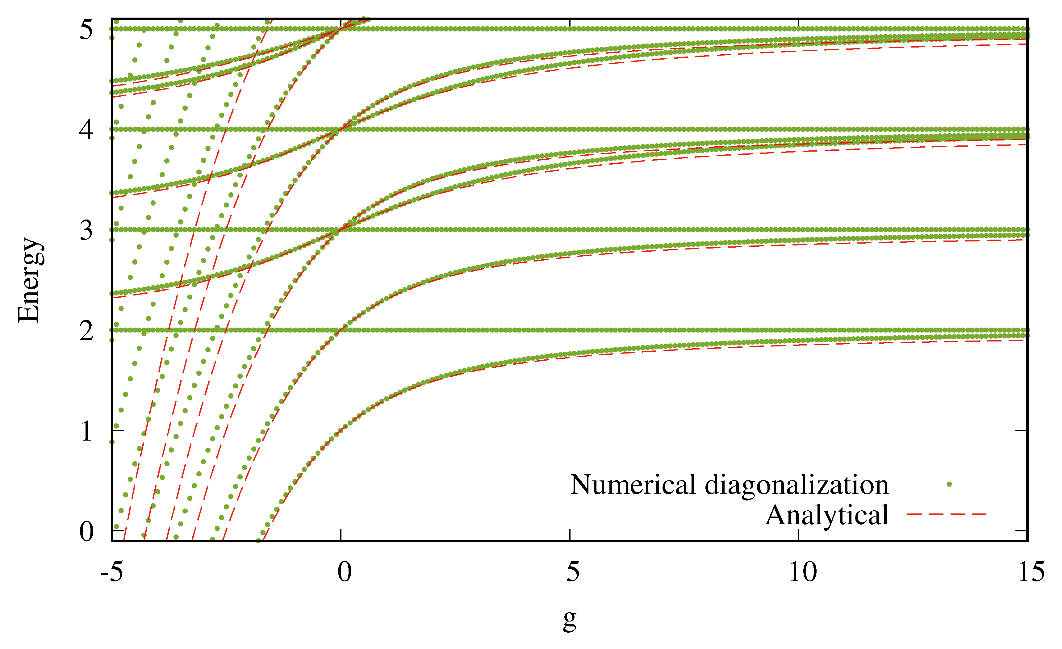
3.3. A Benchmark for the Two-Particle Case

In general, it is not possible to solve exactly the energy spectrum. In our case, to determine the energy spectrum we have to diagonalize the Hamiltonian in a large Hilbert space by using sophisticated numerical techniques. However the case of two particles has been analytically solved in the literature [44].

3.3.1. Theoretical Spectrum for Two Particles

For two fermions with opposite spin, $M=0$, the energies of the relative motion are obtained by solving the transcendental equation [44]

$$\frac{\Gamma (-E_r/2+3/4)}{\Gamma (-E_r/2+1/4)}=-\frac{g}{2^{3/2}},$$

(43)

where $\Gamma$ are gamma functions, $E_r$ is the energy of the relative system and g is the interaction strength.

In addition, the center-of-mass motion is governed by an harmonic oscillator Hamiltonian Equation (8), and its energy is given by Equation (3). Then, the energy of a two-body state is the sum of its relative and center-of-mass energies. Therefore, each relative state has its corresponding center-of-mass excitations.

These analytical results are used as a test for our numerical calculations and allow us to critically analyze the dependence of the numerical results on the size of the Fock subspace used in the diagonalization. As g increases one needs a larger subspace.

3.3.2. Comparison of Analytical and Numerical Results

In Figure 1 we report as a function of g the low-energy part of the two-particle energy spectrum calculated by diagonalization in a truncated basis space (green dots) and the spectrum obtained by solving Equation (43). Notice that this equation provides the energies of the relative motion to which we add the possible energies of the center of mass: $E_{CM}$. For the ground state, $E_{CM}=1/2$. On the contrary, the diagonalization provides the total energies of the system. The diagonalization has been performed using 100 single-particle modes that translates when the energy restriction is taken into account into a dimension of 5050 of the matrix to be diagonalized.

We explore both the attractive and the repulsive interaction regimes. In general, for small values of $|g|$, both attractive and repulsive, the agreement between both types of calculations is very good. Apparently, the quality of the results deteriorates faster for attractive interaction. The calculations discussed in this paper will consider mainly repulsive interactions which will be explored up to the interaction strength limit which is almost reached for the highest values of g considered, $g=15$.

In the plot, we also include the horizontal lines which are energies of states not affected by the interaction. The first one corresponds to the state with $S=1$ and $M=1$ whose wave function can be decomposed as an antisymmetric wave function in coordinate space built with the single-particle states: $n=0,1$ times the triplet spin state with $M=1$. The energy of this state, $E=2$, does not depend on g. In fact, all the states described by horizontal lines in the figure, are eigenstates of the Hamiltonian with $M=1$. Notice also that in the limit $g\to \infty$ states with $M=0$ become degenerate with states with $M=1$.

To complete the study of the accuracy of our calculations we investigate the convergence of the energy of the ground state and first excited state of the two particle system as a function of the number of harmonic oscillator modes used ($N_M$). Note that for $N=2$, the energy constraint for the construction of the two-body basis is given by the maximum energy $E_{\max }=1/2+(N_M-1/2)=N_M$.

To this end, in Figure 2 we report the difference between the ground-state energy obtained by the diagonalization procedure and the analytical ones, for two values of the interaction strength. The figure also reports the difference of the first excited state. For $N=2$, it is possible to establish the dependence of the dimension of the Hilbert space on $N_M$, which is given by $N_M(N_M+1)/2$. As expected, the difference between the calculated and the exact value decreases with the number of modes. Following Ref. [53], we fit functions of the type $C_1/N_M^{1/2}+C_2/N_M$ with excellent results. In addition, for large values of $N_M$, the convergence of the energy goes as $1/N_M^{1/2}$. This dependence indicates a slow convergence of the numerical results by increasing the number of single-particle modes. As expected, the differences are larger for the larger strength, but in both cases the differences are very small. In all cases the difference is positive, indicating that the numerical results are upper bounds to the exact ones.

4. Ground State Properties

In this section we discuss and analyze different observables characterizing the ground state of the system. This analysis is done for several numbers of particles and total spin projections, devoting special attention to the two-particle system, as it is the only one with analytical solution.

As the interaction is spin independent, the Hamiltonian for a given number of particles is calculated in a subspace with a well-defined total spin projection M. After diagonalization of the Hamiltonian, the lowest eigenvalue and its corresponding eigenvector is identified as the ground state of the system for this spin projection.

The ground state is written in the Fock basis as

$$|\Psi \rangle =\sum _n{C}_n|{\psi }_n\rangle ,$$

(44)

where $|{\psi }_n\rangle$ is a vector of the many-body basis of the Fock space, all with the same spin projection and constructed with the single particle eigenstates of the harmonic oscillator.

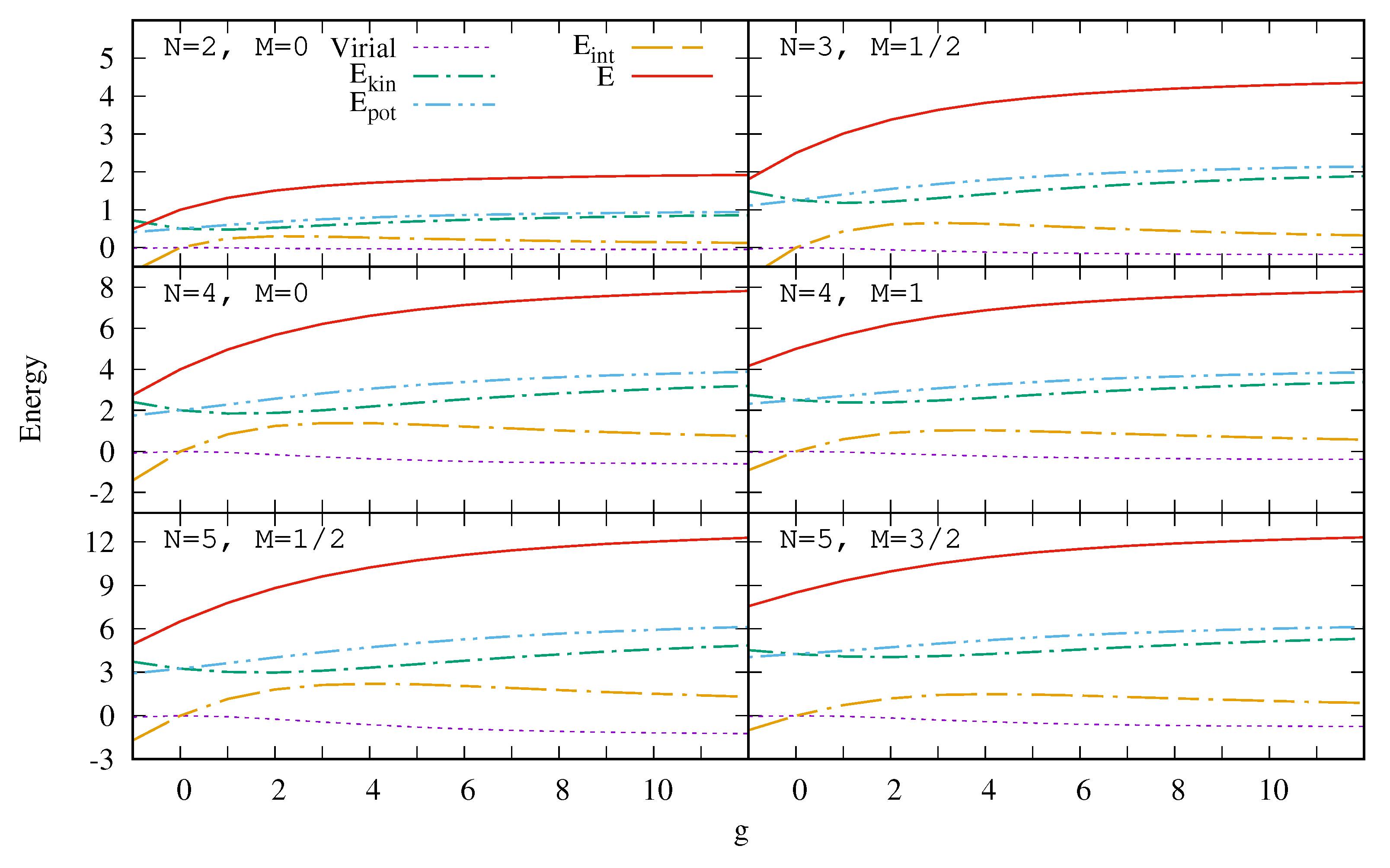
4.1. Energy and Virial Theorem

The energy of the ground-state as a function of the interaction strength g for several number of particles and spin configurations is shown in Figure 3. The first thing to observe is that for each number of particles the states with maximum spin projection are not affected by the interaction. In fact, the wave function of these states can be factorized as a symmetric spin function, with all spins up and an antisymmetric spatial wave function. Due to the Pauli principle, this spatial wave function is built with the first N single-particle harmonic oscillator states. As discussed in Section 2 its energy is given by $E=N^2/2$. In all other cases, the ground-state energy grows when g increases and tends to saturate when $g\to \infty$. More precisely, for the $N=2$, $M=0$, the energy evolves from $E=1$ at $g=0$, to $E=2$ in the limit $g\to \infty$. Later in this section, we will discuss the structure of both the spatial and the spin part of the wave function in both limits. For $N=3$, $M=1/2$ the energy goes from $E=5/2$, to the $E=9/2$ for $g\to \infty$. In a similar way, for $N=4$, $M=0$ the energy goes from $E=4$ at $g=0$ to $E=8$ at $g\to \infty$ while for $N=4$, $M=1$ the energy goes from $E=5$ to $E=8$. Notice that in the limit $g\to \infty$ the energy depends only on the number of particles and it is the same for the different spin projections. The values of the energy at $g\to \infty$ were predicted by Equation (14), $E={(N_d+N_u)}^2/2$ where $N_d$ and $N_u$ are the number of particles with spin up and down respectively. On the other hand, in the case of an attractive interaction, the binding energy increases as the interaction becomes more attractive. In this case the energies belonging to different number of particles cross in the figure, as the systems with more particles can accumulate more attraction.

In Figure 3 we also show the results for the cases $N=3$, $M=1/2$, $N=4$, $M=0$ and $N=4$, $M=1$ reported in Ref. [54] for the repulsive regime. For small interaction strengths, $g\lesssim 5$, both calculations agree fairly well, but for larger interactions we can appreciate that our calculations provide larger energy values due to the use of a truncated basis. This effect is more pronounced in the four particles case, which is performed with less harmonic oscillator single-particle states.

After this general view of the dependence of the ground-state energy on the strength of the interaction for different systems, we are going to analyse in more detail the two-particle system with $M=0$, which energy as a function of g is plotted in Figure 3. In the non-interacting case, the wave function can be factorized

$${\Psi }_{g=0}(1,2)={\Phi }_0\left(x_1\right){\Phi }_0\left(x_2\right)\chi (S=0,M=0),$$

(45)

as a symmetric function in space with both particles in the same single-particle state and the two-body spin function corresponding to a singlet state which is antisymmetric: then the total wave function is antisymmetric and its energy is $E=1$. In the limit of a very strong interaction, the wave function can be factorized as [3]

$${\Psi }_{g=\infty }(1,2)=\frac{1}{\sqrt{2}}|{\Phi }_0\left(x_1\right){\Phi }_1\left(x_2\right)-{\Phi }_1\left(x_1\right){\Phi }_0\left(x_2\right)|\chi (S=0,M=0)$$

(46)

i.e., the absolute value of the determinant built with the ground and first excited single-particle states of the confining harmonic oscillator times the singlet two-particle spin function. In this case, the presence of the absolute value ensures that the spatial part of the wave function is symmetric. Notice also that this wave function does not allow two particles to be at the same position and therefore the two particles do not feel the interaction. The final energy of this wave function is the sum of the single-particle energies, $E=1/2+3/2=2$. However, even if the wave function of Equation (46) looks rather simple, due to symmetry arguments, the diagonalization procedure requires a very large Fock space to asymptotically approach the solution.

It is also interesting to study the decomposition of the energy in different pieces: kinetic, harmonic-oscillator potential energy and interaction energy, which are constrained by the virial relation:

$$2\langle T\rangle -2\langle V_{\mathrm{ho}}\rangle +\langle V_{\mathrm{int}}\rangle =0.$$

(47)

The fulfilment of this relation reinforces the accuracy of the calculations. The derivation of the virial relation can be found in the Appendix A, and the evaluation of the kinetic energy and the harmonic trapping potential energy in Appendix B.

In Figure 4 we report, as a function of the interaction strength, the different contributions to the ground-state energy, for different number of particles and total third-spin component. The total energy is also reported. In general, for all cases considered, the behavior of the different contributions is rather similar. For a repulsive interaction, the total energy increases. In the repulsive interaction range, both the kinetic energy and the oscillator-potential energy are similar. Actually, they are equal at $g=0$ and also tend to the same value in the limit of infinite interaction. The oscillator-potential energy is greater than the kinetic energy in this range. The interaction energy starts from zero in the non-interacting case, has a maximum, and goes to zero as the interaction strength tends to infinity.

Obviously, the virial theorem is trivially respected for the systems with maximum spin projection, as in these cases the interaction energy is zero and therefore the kinetic and harmonic potential energy coincide. In general the virial theorem is well fulfilled, although it deteriorates a little when the interaction strength is increased. The behavior of the different contributions to the total energy can be explained by taking into account the virial theorem and knowing the non-interacting and infinite-interacting limits. In the non-interacting case, the kinetic energy is equal to the oscillator potential energy. In the infinite interaction limit, the wave function is given by Equation (46), that prevents two particles from having the same position, therefore, the interaction energy is zero. As a consequence, the kinetic and the harmonic oscillator energies are also equal and fulfill the virial relation. For intermediate interactions, the interaction energy is positive, and the kinetic energy is lower than the oscillator-potential energy in agreement with the virial theorem. The continuity of the interaction energy between zero and infinite interaction allows us to predict the existence of a maximum of the interaction energy as a function of g. On the other hand, when the interaction is attractive, the interaction energy takes negative values, increasing the binding energy as the interaction becomes more attractive. At the same time, the kinetic energy grows and the harmonic potential energy decreases, as a consequence of the decrease of the size of the system.

4.2. One Body Density Matrix

The one-body density matrix (OBDM) provides a non-trivial insight on the many-body structure of the system. The OBDM allows one to obtain the natural orbits, i.e., the eigenvectors of the OBDM, the momentum distribution and the density profile of the system. In second quantization, the matrix elements of the OBDM associated to $|\Psi \rangle$ are defined as,

$${\rho }_{ij}=\langle \Psi |a_j^{†}{a}_i|\Psi \rangle =\sum _{n,m}{C}_n^{*}{C}_m\langle {\psi }_n|a_j^{†}{a}_i|{\psi }_m\rangle .$$

(48)

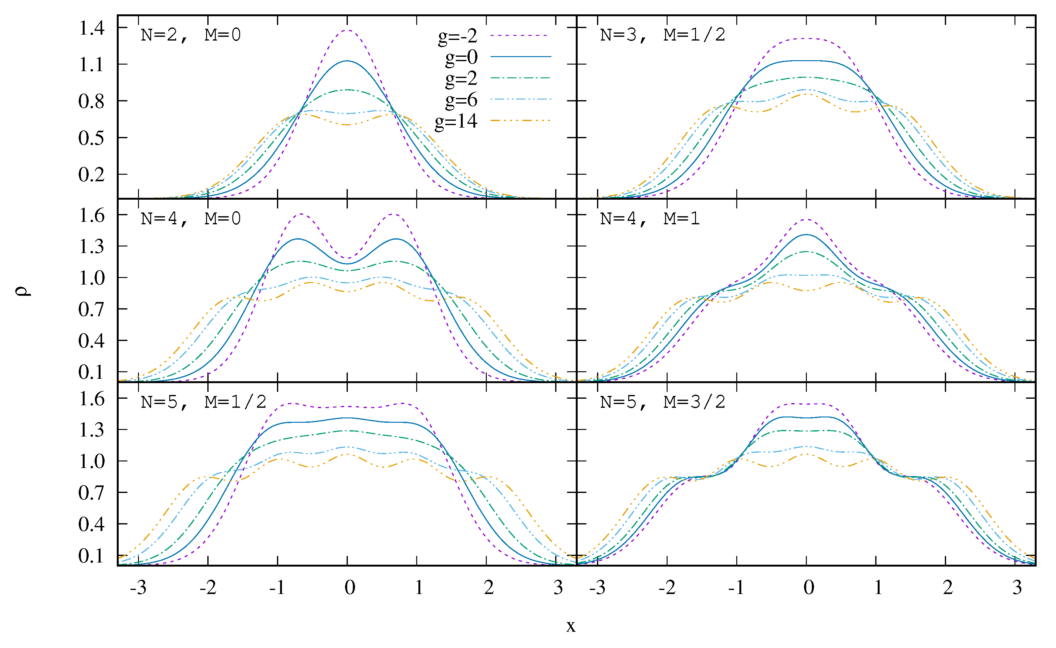
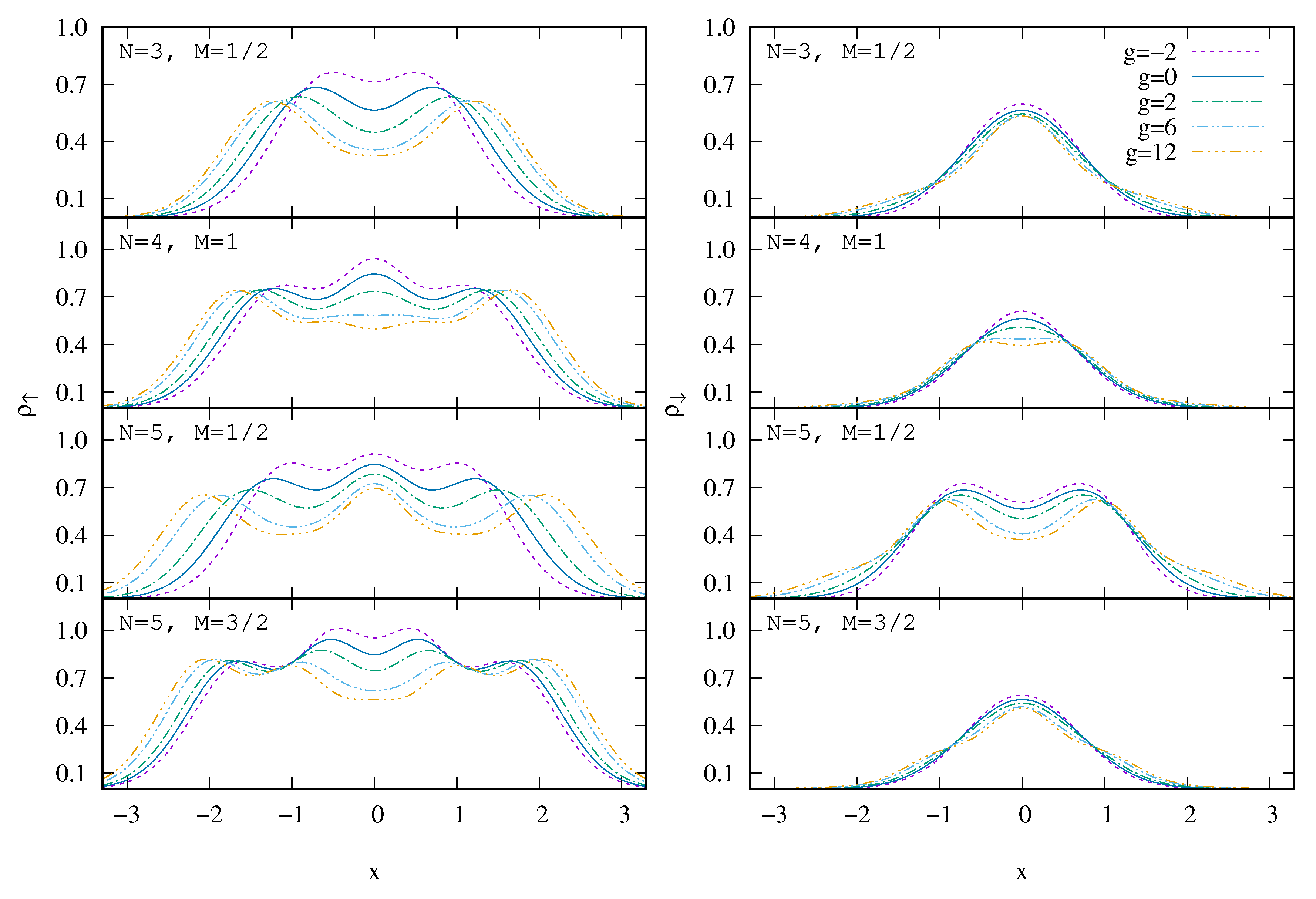
4.2.1. Density Profile

The first observable to be calculated is the density profile of the ground state of the system, that provides information on how the particles are spatially distributed in the trap.

The density profile in terms of the matrix elements of the OBDM is given by,

$$\rho \left(x\right)=\sum _{i,j}{\Phi }_i^{*}\left(x\right){\rho }_{ij}{\Phi }_j\left(x\right),$$

(49)

where ${\Phi }_n\left(x\right)$ are the single-particle wave functions used to construct the many-body basis. This expression corresponds to the diagonal elements of the one-body density matrix in spatial representation.

In Figure 5 we report the density profile of the ground state of the system for different number of particles and spin configurations and for several values of the interaction strength. As expected, the density profiles at $g=0$ for the different systems fully agree with the analytical expressions given in Equation (12). For large values of g, $g=14$ in the figure, the density profiles are very close to the ones predicted in Equation (15). The small differences are due to the finite value of g and also to the finite size of the Hilbert space where we are diagonalizing the Hamiltonian. In any case, both for the energy and the spatial distribution of the particles, $g=14$ can be considered a strongly interacting regime. Notice, that for the same number of particles and different spin configurations the density profiles are rather different, when g is small. However, for $g\to \infty$ the profile for a given number of particles does not depend on the spin projection. In the strongly interacting limit, the density profile shows as many peaks as the number of particles, i.e., the particles try to be distributed equidistantly to minimize the repulsion. The size of the system also increases with the interaction strength. For attractive interactions, $g=-2$ is shown in the figure, the density profile is narrower and reaches higher values than in the repulsive case.

In Figure 6 we report the densities of the spin up and spin down particles. The cases $N=2$, $M=0$ and $N=4$, $M=0$ are not reported, because these cases have the same particles with spin up and spin down, and for symmetry reasons, the densities of both types of particles are equal and these cases do not provide new information. For the remaining cases, we can see that in every density profile there are the same number of peaks as particles with the correspondent spin projection. As the interaction increases, the peaks separate to mimimize the interaction energy.

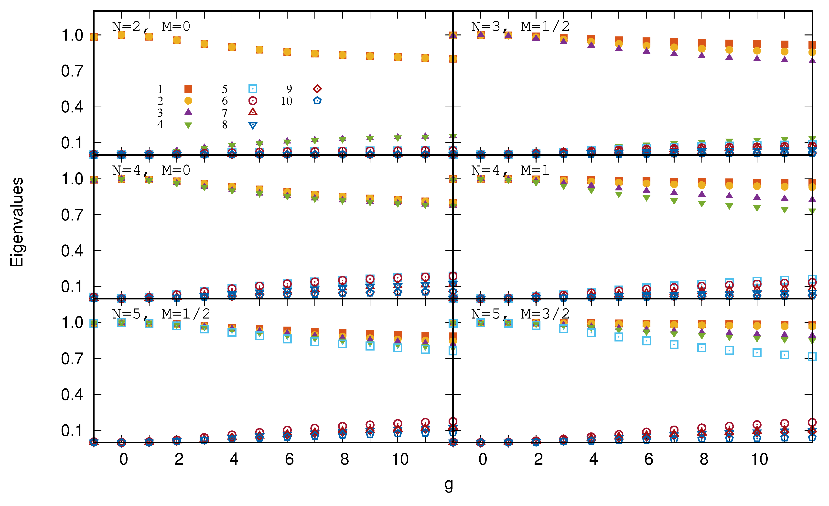
4.2.2. Natural Orbits

The diagonalization of the density matrix provides its eigenvectors, i.e., natural orbits, and its eigenvalues, which can be interpreted as the occupation number of the natural orbits. The sum of the eigenvalues of the natural orbits is normalized to the total number of particles.

In the non-interacting case, the ground state of an N-particle system, which corresponds to a Slater determinant built with N single-particle harmonic oscillator functions with their spin projection, produces an OBDM with N-natural orbits with eigenvalue 1 and the all others with eigenvalue zero. In these cases the natural orbits can be identified with the single-particle wave functions used in the construction of the Slater determinant. When turning on the interaction, one gets a set of N-natural orbits with eigenvalues smaller than 1 and additional natural orbits with eigenvalues significantly smaller. The natural orbits are expressed as linear combinations of the harmonic oscillator single-particle basis and the Slater determinant built with the N natural orbits with the highest eigenvalues define the wave function of this type with largest overlap with the ground state. However, this condition does not imply that the energy corresponding to this wave function is the minimum energy for a wave function built with a single Slater determinant. The fact that the OBDM has eigenvalues smaller than 1 points out the existence of correlations beyond the mean-field in the ground-state of the system which translate into the impossibility to express the ground-state wave function as a single Slater determinant of single-particle wave functions.

The eigenvalues associated to the natural orbits can be interpreted as the occupation numbers of the single-particle states defined by the natural orbits. Notice also that a given natural orbit does not mix single particle states with different parity or spin projection.

In Figure 7 we report the dependence of the ten largest eigenvalues of the one-body density matrix as a function of the interaction strength for the ground-state of systems with different number of particles and spin projections. As explained above, at $g=0$ we have N, where N is the number of particles, eigenvalues equal to unity, and the rest equal to zero. When the interaction increases, the highest eigenvalues decrease indicating the presence of correlations in the system. Then as the eigenvalues are normalized to N, the smaller eigenvalues start to increase, indicating the impossibility to describe the wave function with only one Slater determinant. The fact that the eigenvalues of the OBDM could be the same, does not necessarily imply that the natural orbits are the same. However, for $N=2$ and $M=0$ the eigenvalues appear doubly degenerate independently of the value of g. One corresponds to spin up and the other to spin down that have identical natural orbits and also the same spatial distribution. The same is true for the $N=4$ and $M=0$ case. For $g=0$ we have four natural orbits, two corresponding to the single-particle state $n=0$, both with spin up and spin down and the other to $n=1$ also with both spin projections, all with eigenvalue equal to unity. Then when the interaction increases, the natural orbits mix higher excited harmonic oscillator states but do not mix the spin projection. The natural orbits are independent of the spin projection and the eigenvalues separate in two groups each one with degeneracy two. They have not only the same eigenvalue but also the same spatial structure. Instead, for $N=3$ and $M=1/2$ the natural orbits of each spin projection are different.

The reason behind the previous observations is that the OBDM is constructed in boxes of well defined third spin component,

$$\left(\begin{array}{cc}\hfill {\rho }_{\uparrow \uparrow }& {\rho }_{\downarrow \uparrow }\hfill \\ \hfill {\rho }_{\uparrow \downarrow }& {\rho }_{\downarrow \downarrow }\hfill \end{array}\right)=\sum _{n,m}{C}_n^{*}{C}_m\langle {\psi }_n|\left(\begin{array}{cc}\hfill a_{\uparrow }^{†}{a}_{\uparrow }& a_{\downarrow }^{†}{a}_{\uparrow }\hfill \\ \hfill a_{\downarrow }^{†}{a}_{\uparrow }& a_{\downarrow }^{†}{a}_{\downarrow }\hfill \end{array}\right)|{\psi }_m\rangle .$$

(50)

However, the crossed terms are zero and only the diagonal terms contribute. Therefore the matrix separates in two pieces, one with spin up and the other with spin down. If the system is symmetric in the third spin component, both subspaces are equal and the eigenvalues and spatial eigenfunctions of each subspace are also equal.

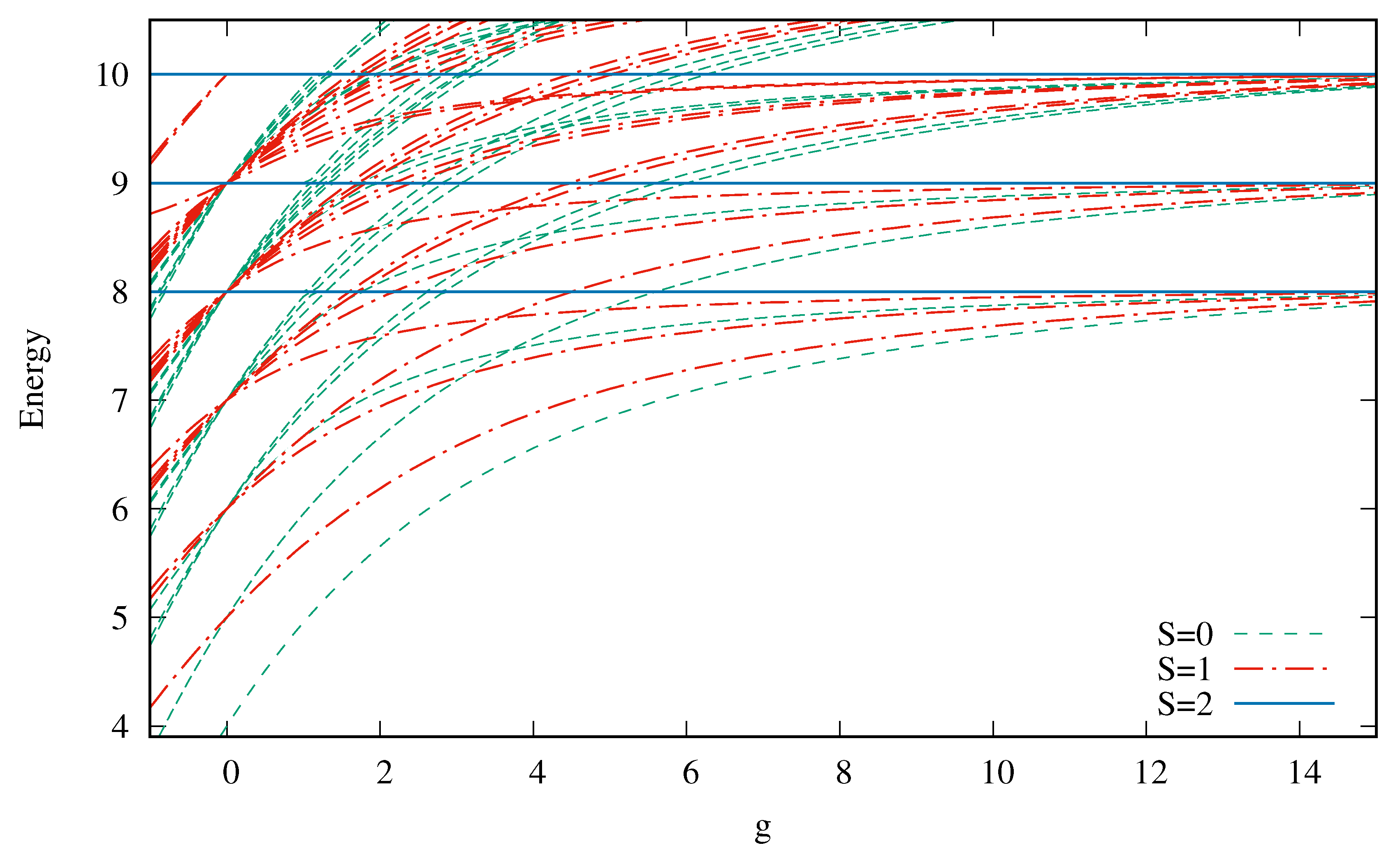
5. Low-Energy Excited States

To complete the study of the structure of the few-body fermion systems, in this section we discuss the low energy excitation spectrum which will be useful to understand the dynamics and the response of the system to an external perturbation. In this section we present an algorithmic procedure to assign quantum labels to the different states, a more formal study of the symmetries in few-atom systems with examples for three to five atoms is given in Ref. [32].

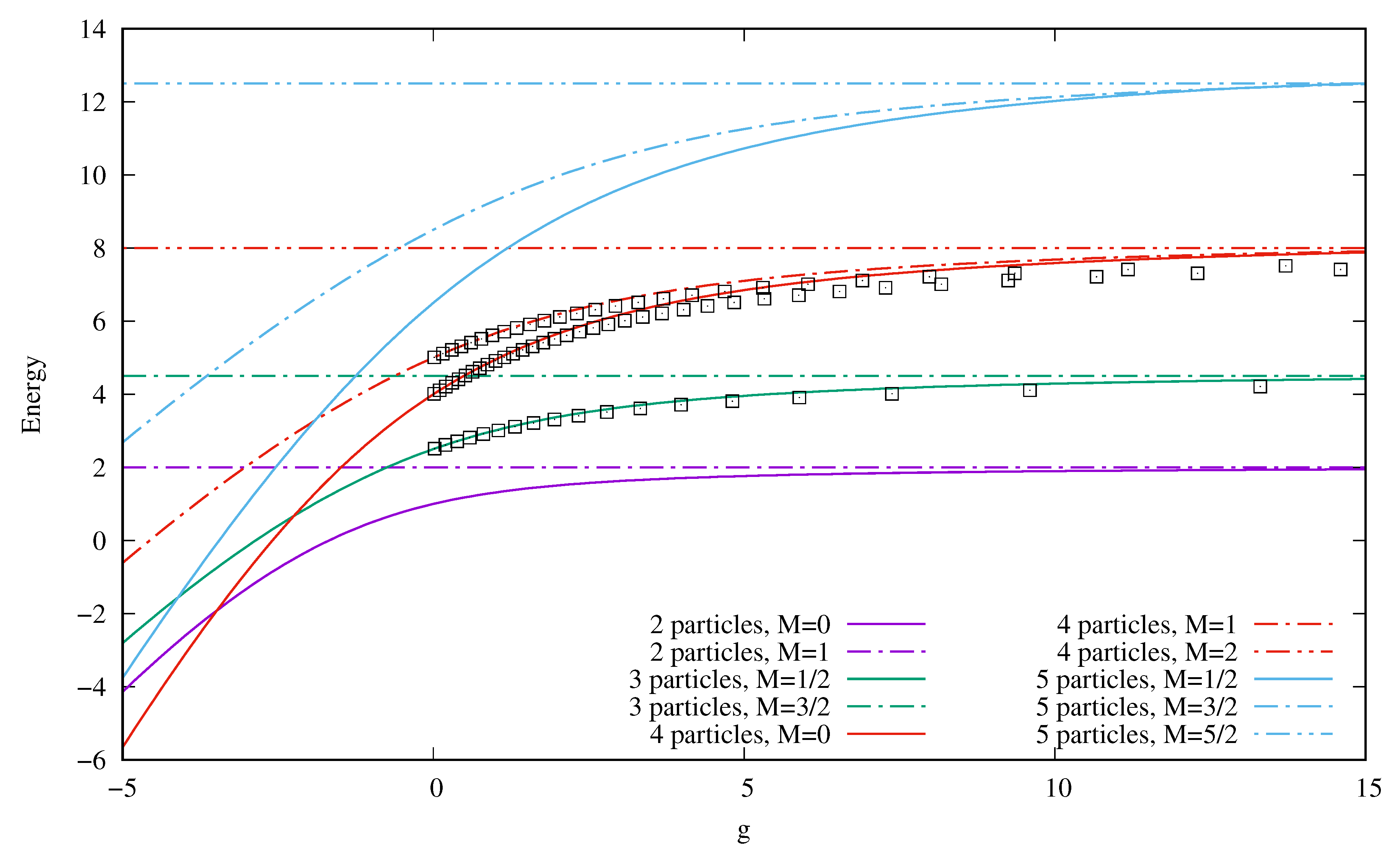
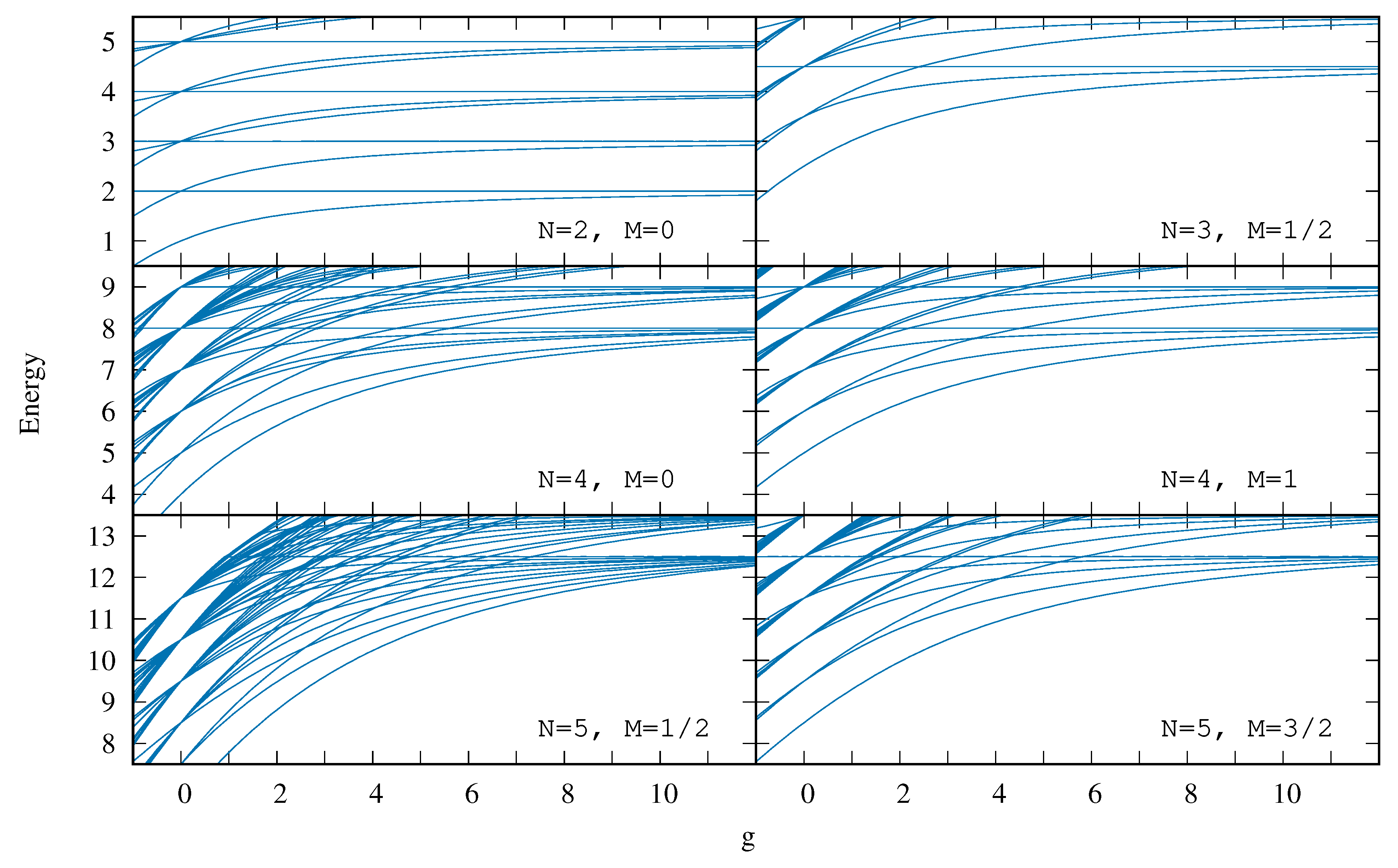
5.1. Energy Spectrum

Once the Hamiltonian for a given number of particles (N) and total third spin component (M) has been diagonalized, we have access to the spectrum and the structure of the eigenstates. We pay particular attention to the dependence on the interaction strength of the low-energy part of the spectrum, which is shown in Figure 8 for several particles and spin configurations.

The first observation is the existence of states which are not affected by the interaction and therefore appear as horizontal lines in the plots. These states correspond to antisymmetric wave functions in space and give zero probability of having two particles in the same position. Actually, these wave functions can be factorized in an antisymmetric wave function in space and a spin symmetric wave function. Later on, in Section 5.2 we discuss how to assign the total spin quantum number to the different eigenstates.

Another general observation is the existence of excitations with a constant energy shift independent of the interaction strength which is associated to excitations of the center of mass of the system. Notice that the interaction which is invariant under space translations does not affect the center-of-mass motion.

An interesting feature is that the energy of all states saturates when the interaction strength tends to infinity. Actually, some states merge to the same energy when $g\to \infty$ increasing the degeneracy of the energy levels in this limit.

Once more, let us analyze more carefully the case $N=2$ and $M=0$. As explained in the previous section, the non-interacting ground state corresponds to

$$\Psi (1,2)={\Phi }_0\left(x_1\right){\Phi }_0\left(x_2\right)\chi (S=0,M=0),$$

(51)

with energy $E=1$. The two first excited levels have the same energy, $E=2$ at $g=0$, one corresponds to a state

$$\Psi (1,2)=\frac{1}{\sqrt{2}}({\Phi }_0\left(x_1\right){\Phi }_1\left(x_2\right)-{\Phi }_1\left(x_1\right){\Phi }_0\left(x_2\right))\chi (S=1,M=0),$$

(52)

which is a product of an antisymmetric function in coordinate space and a symmetric one in spin. This state is not affected by the contact interaction and its energy is independent of g. The energy of this state merges with the ground state energy when $g\to \infty$. As the Hamiltonian commutes with the spin, this state is degenerate with states having the same spatial wave function and the spin functions corresponding to $S=1$ but $M=0,\pm 1$.

The other excited state at $g=0$ corresponds to

$$\Psi (1,2)=\frac{1}{\sqrt{2}}({\Phi }_0\left(x_1\right){\Phi }_1\left(x_2\right)+{\Phi }_1\left(x_1\right){\Phi }_0\left(x_2\right))\chi (S=0,M=0),$$

(53)

which is symmetric in spatial coordinates and antisymmetric in spin. It can be shown that this state corresponds to the first excitation of the center of mass times the intrinsic wave function of the ground state described above. In the ground state, the center of mass is always in the ground state of $H_{\mathrm{CM}}$. However, in the state we are considering the center of mass occupies the first excited state of $H_{\mathrm{CM}}$. This is true for all values of g and the energy of this state can be written as $E=E_{g.s.}+1$ for all values of g. This state has degeneracy one. Actually, the wave function of this state can be written as the ground-state wave function at a given g times the wave function of the first excited state of $H_{\mathrm{CM}}$.

This type of arguments explain the full spectrum for $N=2$. It is worth reminding that our numerical procedure is constructed in the Fock space using single-particle wave functions, without decomposing the Hamiltonian in the center of mass and intrinsic parts. Therefore the proper localization of the center of mass excitations provides a test on the numerical accuracy of the calculations.

We continue our analysis by considering the case for $N=3$ and $M=1/2$. The ground state at $g=0$ has an energy $E=1/2+1/2+3/2=5/2$, which corresponds to a state that populates the single-particle harmonic-oscillator states: $\{0\uparrow ,0\downarrow ,1\uparrow \}$, that results in $M=1/2$. Then when g increases, the state mixes more complicated configurations, the energy increases monotonously and tends to $E_{g\to \infty }=1/2+3/2+5/2=9/2$. The spin of the ground state is $S=1/2$, which is the minimum compatible with the value of $M=1/2$ and its parity is negative all along the values of g. At $g\to \infty$ the ground state merges with the state with $S=3/2,M=1/2$ which is a state built with a Slater determinant with the single-particle harmonic-oscillator states: $n=0,1,2$ times the symmetric wave function of three spins $S=3/2,M=1/2$. The particles in this state do not feel a contact interaction and the energy of this state is independent of the interaction strength. Notice also the existence of two states at $g=0$ with $M=1/2$ built with the single-particle harmonic-oscillator states $\{0\uparrow ,0\downarrow ,2\uparrow \}$ and $\{0\uparrow ,1\downarrow ,1\uparrow \}$ which give origin at $g=0$ to two states with total energy $E=7/2$. One describes an excitation of the center of mass built on top of the ground state which evolves with g keeping always the same energy shift respect to the ground state, and the other state merges with the ground state when $g\to \infty$.

Next, we discuss the case $N=4$ and $M=0$. Of course, the number of levels increases with the number of particles and the number of levels is larger when the total spin projection, M is smaller. One immediately detects states not affected by the interaction. In particular, the lowest one that corresponds to a state with $S=2$, the maximum spin for $N=4$ and $M=0$. This state is described by a wave function that is the product of an antisymmetric wave function given by a Slater determinant built with the single-particle harmonic-oscillator states: $n=0,1,2,3$ and a symmetric spin function of four particles with $S=2$ and $M=0$. The total energy of this state, $E=1/2+3/2+5/2+7/2=8$, is given by the sum of the first four single-particle energies of the harmonic-oscillator trapping potential.

The ground state is a state with $S=0$, i.e., the minimum total spin compatible with the value of M. The energy of the state at $g=0$, $E=4$, corresponds to the occupation of the single particle levels: $\{0\uparrow ,0\downarrow ,1\uparrow ,1\downarrow \}$. The energy gets more repulsive as g increases and for $g\to \infty$ the energy merges with the energy $E=8$ of the previously discussed state. The parity of the ground-state is positive. One can also identify the excitations of the center of mass characterized by a constant shift of the energy respect to the ground-state or on top of a given state. For instance, the first one corresponds to a center of mass excitation of one unit of energy of the Hamiltonian associated to the center of mass, $H_{\mathrm{CM}}$. There are other levels whose quantum numbers can be identified and many of them merge together when $g\to \infty$.

Similar comments apply to the case $N=4,M=1$. One can also identify states not affected by the interaction. In particular, the lowest one corresponds to $S=2,M=1$, that has the same energy as the state $S=2,M=0$ of the previous panel. Actually, both states $S=2,M=1$ and $S=2,M=0$ can be built from the state $S=2,M=2$ constructed with an antisymmetric space wave function times a symmetric spin wave function with all spins up. These states are obtained by applying the ladder operator $S_{-}$ to the state $S=2,M=2$. When the Hamiltonian commutes with $S_{-}$ this operation does not change the energy of the state. These arguments are discussed at length in Section 5.2. In this $M-$box, the ground state starts with $E=5$ at $g=0$ which corresponds to the Slater determinant built with the single-particle states: $\{0\uparrow ,0\downarrow ,1\uparrow ,2\uparrow \}$ and when $g\to \infty$ merges with several states that tend to $E=1/2+3/2+5/2+7/2=8$.

Finally let us discuss very briefly the case $N=5,S=1/2$. In this case, there are many levels below the first level which is not sensitive to the interaction strength, with an energy $E=1/2+3/2+5/2+7/2+9/2=25/2$ and $S=5/2,M=1/2$. The ground state, has $S=1/2$, and positive parity. At $g=0$ it has an energy $E=13/2$ and when $g\to \infty$ it merges with the state that is non-sensitive to the interaction discussed above, with an energy $E=25/2$.

For the case with $M=3/2$ there are considerably fewer levels. The ground state at $g=0$ has more energy than the ground state for $M=1/2$, basically due to the Pauli principle. In fact, at $g=0$ the ground-state is built with the single particle states $\{0\uparrow ,0\downarrow ,1\uparrow ,2\uparrow ,3\uparrow \}$, which gives an energy $E=17/2$. However, when g is increased the state merges with the state $S=5/2,M=3/2$ which is also degenerate with the sate $S=5/2,M=1/2$ discussed in the previous panel.

Whenever possible, we have compared our results with the ones provided in Ref. [33] obtaining a good agreement in all cases considered. In fact our results, which provide upper bounds, are in general slightly below the results of Ref. [33].

Finally, let us point out that in the limit of large interaction several groups of states merge to the same energy giving rise to an increase of the energy degeneracy. In particular, for the ground state this degeneracy is expressed as $D=\frac{N!}{N_u!N_d!}$.

5.2. Spin Determination

As the Hamiltonian does not depend on the spin, it commutes with the spin operators and should be possible to assign a total spin to the eigenstates of the Hamiltonian. In particular, it commutes with the ladder lowering $S_{-}$ and raising $S_{+}$ spin operators. Therefore, if we have a state with a total spin S and spin projection M with energy E, due to the commutation relations of $S_{+(-)}$ with the Hamiltonian, it turns out that by applying the operators $S_{+(-)}$ to this state one obtains a state with the total spin projection increased (reduced) by 1, i.e., $M\pm 1$, with the same energy E. Therefore, for each eigenstate with a well-defined spin, there will be $2S+1$ states with the same energy. We can use this fact to determine the total spin of the states. The argument is as follows: Given N fermions, we start considering the maximum possible spin projection, that will be the state with all spins pointing up, with $M=N/2$. In this case, the wave function factorizes in a spatial antisymmetric wave function times a symmetric spin wave function. This wave function has a well defined spin which coincides with the maximum value of the spin projection, $S=N/2$. Then if we apply $2S$ times to this state the operator $S_{-}$, we will get the remaining states belonging to this spin multiplet, all having the same energy and all of them factorized as an antisymmetric wave function in space times a spin symmetric wave function. Obviously, these states are found in different M-box subspaces. In fact, if we consider the Hamiltonian in the box with $M=S-1$, among the energies obtained in this box, we find the previous energy attributed to $S=N/2$, corresponding in this case to the state with $M=N/2-1$.

Besides, if the remaining states in this M-box are not degenerate, one can assume that the total spin of each one will be the minimum S compatible with the value of M, i.e., $S=N/2-1$. One can have more than one state with this spin and one would need another quantum number to distinguish between them. Next, we take the box of the Hamiltonian associated to the value of M, $M=N/2-2$. Here we immediately identify the energies obtained for the previous spin values and again the rest of states have a spin that is the minimum compatible with the value of M. One can continue this process until the total spin projection has the positive lowest half-integer value for odd N or zero value in case of even N.

To illustrate this procedure, we consider the lowest-energy states of the case $N=4$ shown in Figure 9 as a function of the interaction strength. The maximum possible spin projection is $N/2=2$. The wave functions with $S=2$ and $M=2$ can be factorized in an antisymmetric spatial wave function times a spin wave function with all spins pointing up. In particular, the lowest energy for this states ($S=2$ and $M=2$), $E=8$, is the sum of the first four single-particle harmonic oscillator energies, $E=1/2+3/2+5/2+7/2$. In addition, this state is not affected by the interaction and therefore appears as the lowest horizontal line in figure. This energy level corresponds also to the energy of the different possible $2S+1$ states of the $S=2$ multiplet. In the next step we consider the box with $M=1$. First we identify the previous energy and find out several non-degenerate eigenstates which can all be associated to $S=1$ (dot-dashed red lines in the figure). Notice that all of them have different energies, but $S=1$. For instance, at $g=4$ we find three $S=1$ levels with energies below $E=8$. In the next step we diagonalize the subspace with $M=0$ and identify the $M=0$ states corresponding to $S=2$ and to the $S=1$ states detected before. The rest of levels have $S=0$. At $g=5$, we find three $S=0$ levels below $E=8$, all with different energy, and non degenerate. Notice that one of them corresponds to a center of mass excitation and that merges with other levels at $E=9$ when $g\to \infty$. Using these types of arguments one can assign the spin to the eigenstates of the Hamiltonian even if the total wave function could be complicated and most of the times non-factorizable in a spin and a space part.

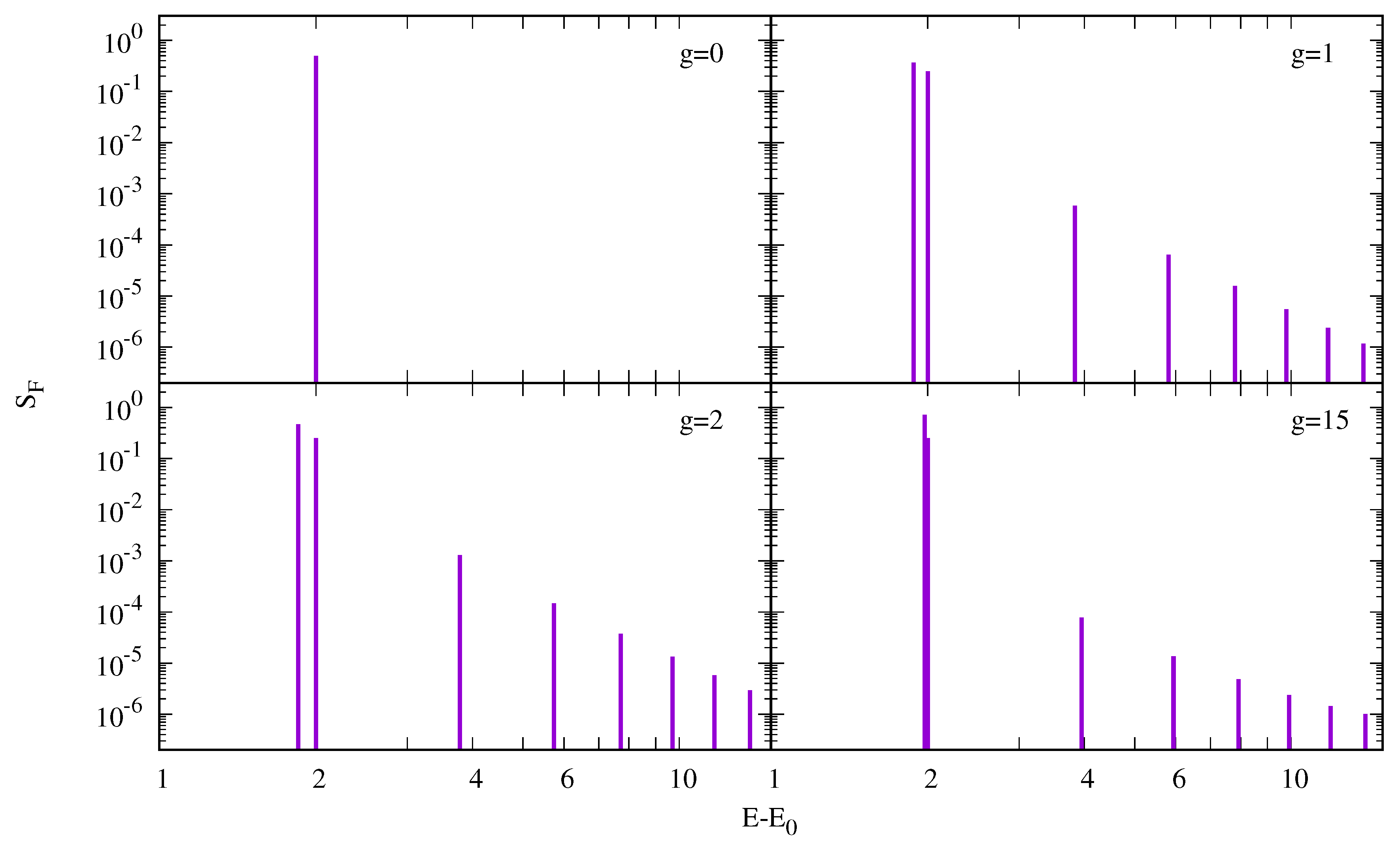
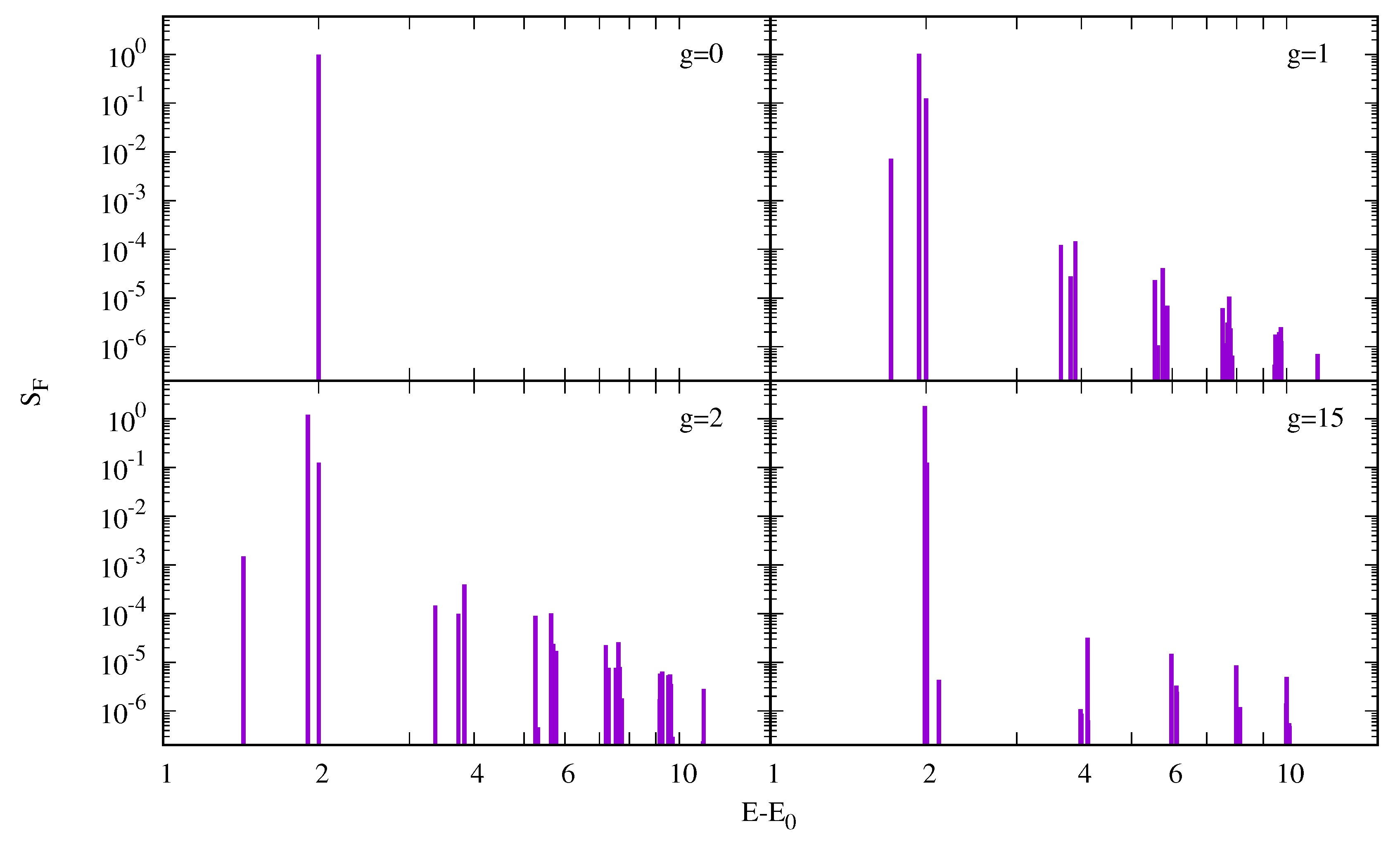
6. Dynamical Excitation

In Section 4 and Section 5 we have concentrated on the static properties of the fermionic system. In particular, we have analyzed the ground state and also the main features of the low-energy spectrum. In the present section we turn our attention to the dynamics of the fermionic system in the harmonic trap. Simulating the dynamics of quantum many-body systems is important for current quantum technological applications where one could for instance design quantum systems to produce desired many-body states after a certain evolution [55,56,57]. A second relevant aspect is that the dynamics of the system reflects in many ways its internal structure. In this sense, one can devise a dynamical evolution in order to unveil the spectral structure of the system [58]. This is the main goal of this section. To this aim we consider two different perturbations to the ground state of the system, which are sensitive to the low-energy spectra presented before. The first is a sudden change in the trap frequency. This perturbation excites both center-of-mass and relative modes of the system and can be analyzed by computing the dynamic structure function. In the second one, we numerically obtain the time evolution of the system after a sudden quench of the interaction strength. In this case, the center-of-mass modes are not excited and we look for traces of the internal structure on the time evolution of the central density of the cloud.

6.1. Sudden Change in the Trap Frequency: Breathing Mode

A well-known way to study the internal structure of a quantum many-body system trapped in a harmonic oscillator is by exciting the so called breathing mode. In contrast with the Kohn (dipole) mode, where the cloud is initially displaced from the minimum of the harmonic potential [59], in our case we study the response of the system to a change in the trapping frequency. For the two particle case there are studies such as [60,61], and using different confining potential such as [62]. The main tool we consider is the dynamic structure function associated to the mono-polar excitation operator

$$\widehat{F}=\sum _j^N{x}_j^2.$$

(54)

This perturbation preserves spin and parity, therefore, it only connects the ground state of the system with other excited states with the same total spin and parity.

This operator can be separated in two pieces: a center-of-mass and an intrinsic one, i.e., $\widehat{F}=N{X}_{\mathrm{CM}}^2+\frac{1}{N}{\sum }_{j<i}{(x_i-x_j)}^2$. The center of mass of the system is described by an harmonic oscillator Hamiltonian, and the wave functions associated to this part are the harmonic oscillator wave functions. Note that this perturbation can excite the center of mass or the intrinsic part, but not both at the same time.

6.1.1. Dynamic Structure Function

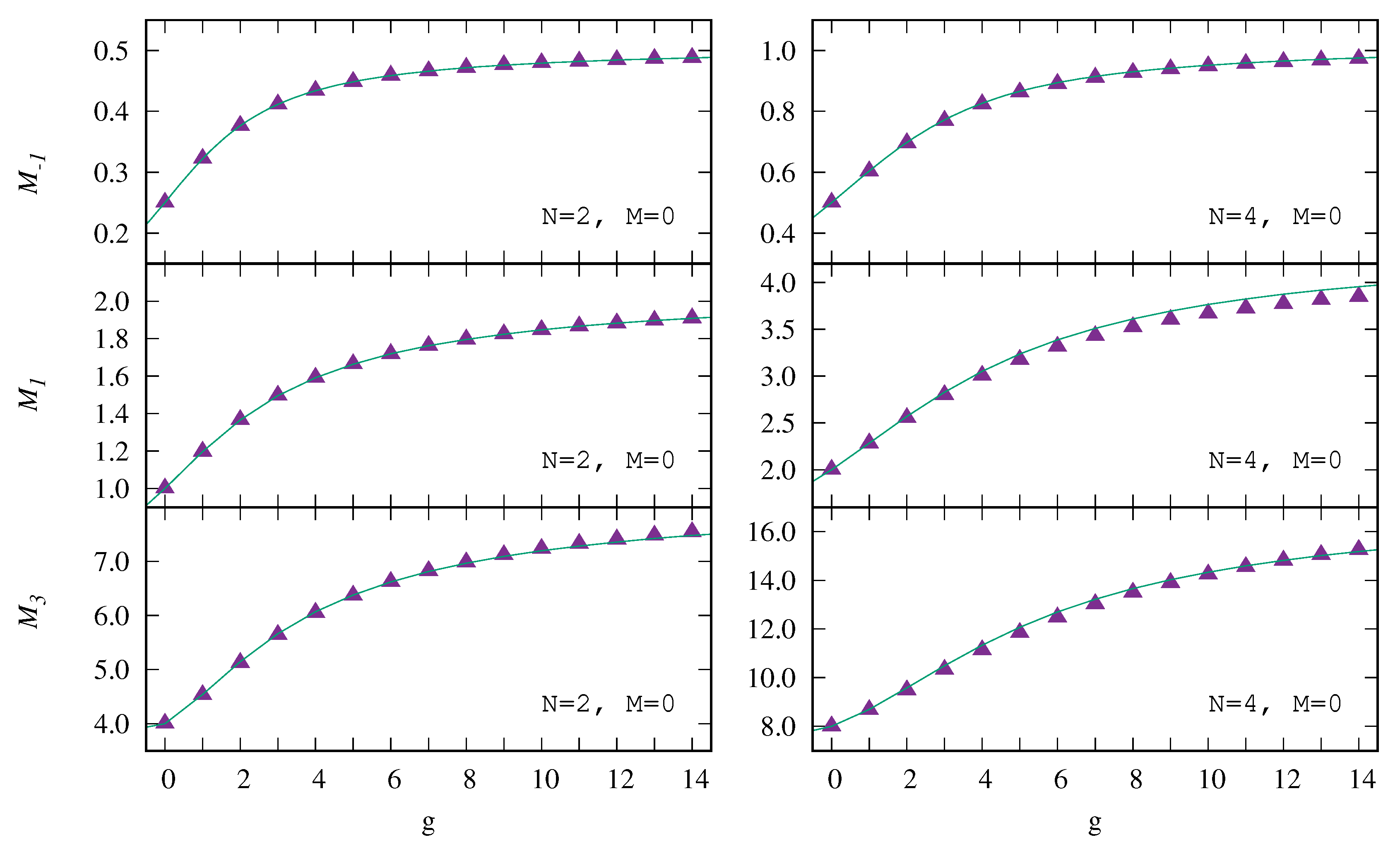
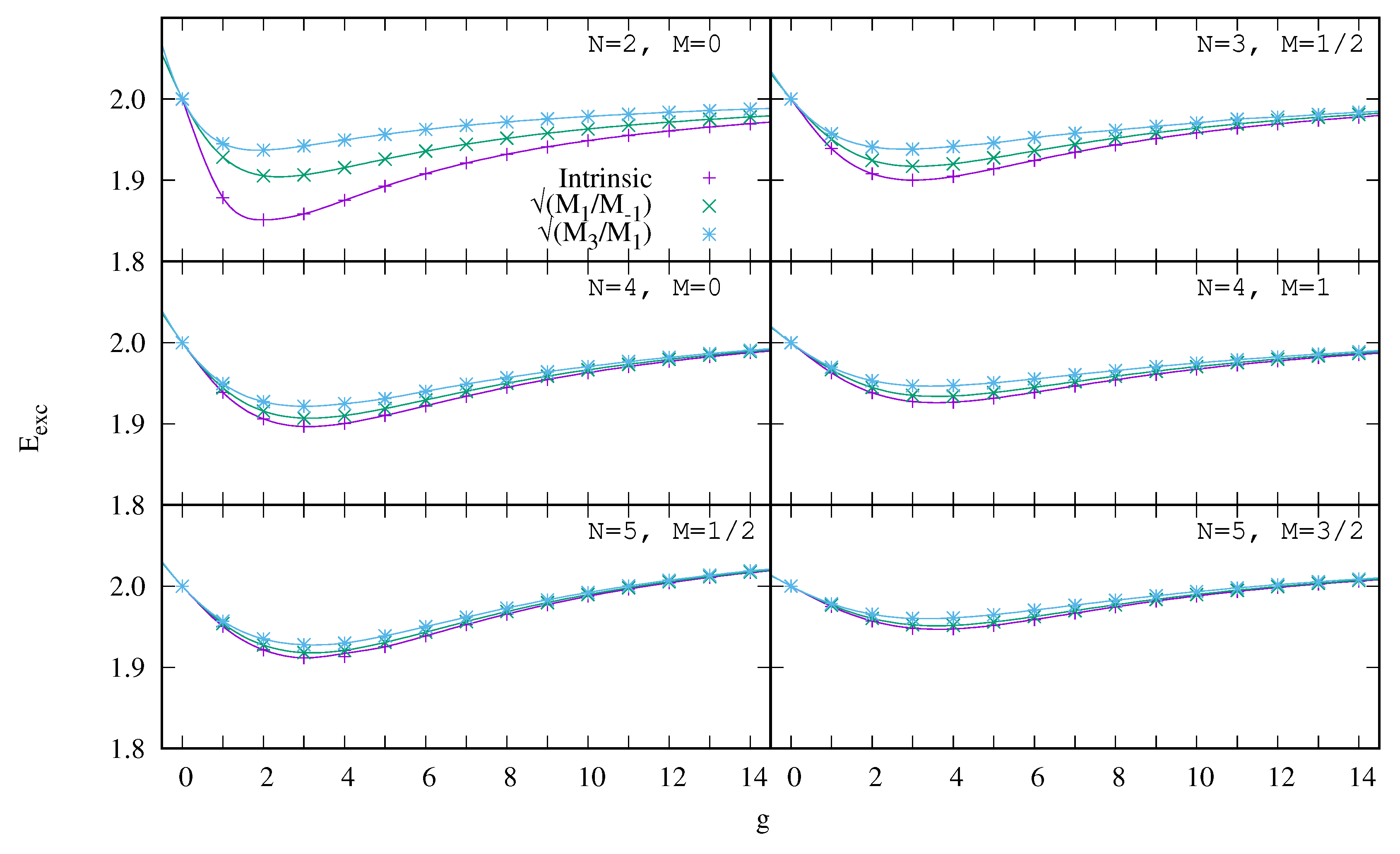
The dynamic structure function, normalized to the number of particles, is defined as

$$S_F\left(E\right)=\frac{1}{N}\sum _{i>0}{|\langle {\Psi }_i|\widehat{F}|{\Psi }_0\rangle |}^2\delta \left(E-(E_i-E_0)\right),$$

(55)

where $\widehat{F}$ is the excitation operator associated to the external perturbation, see Equation (54), $|{\Psi }_0\rangle$ is the ground state of the unperturbed system and $|{\Psi }_i\rangle$ are its excited states.

In the second quantization formalism, the structure function reads,

$$S_F\left(E\right)=\frac{1}{N}\sum _{i>0}{|\sum _{n,m}{C}_{n,0}{C}_{m,i}^{*}\sum _{k,l}\langle k|x^2|l\rangle \langle {\psi }_m|a_k^{†}{a}_l|{\psi }_n\rangle |}^2\delta \left(E-(E_i-E_0)\right),$$

(56)

where |k〉 and |l〉 are harmonic-oscillator single-particle states and $|{\psi }_n\rangle$ are the Fock states of our basis. For the center of mass, the $\langle i_{\mathrm{CM}}|X_{\mathrm{CM}}^2|j_{\mathrm{CM}}\rangle$ are different from zero only when $i_{\mathrm{CM}}=j_{\mathrm{CM}}$ or $i_{\mathrm{CM}}=j_{\mathrm{CM}}\pm 2$. This implies that the center of mass can be excited at most by two energy quanta.

In some limiting cases we know the analytic value of the dynamic structure function. These cases can be used to benchmark our numerical calculations [34]. For the non-interacting case, we expect a single peak in the dynamic structure function with an energy $E-E_0=2$. The intensity of this peak depends on the number of particles and the total spin projection. Likewise, in the infinite interaction limit, we also expect a single peak in the dynamical structure function with energy $E-E_0=2$. In addition, a peak with energy $E-E_0=2$ is expected for any value of the interaction strength, due to the center-of-mass excitation, with a constant intensity as a function of the interaction strength. In the range of repulsive interaction, we expect more peaks associated to states with the same spin and parity as the ground state. These correspond to intrinsic excitations.

In Figure 10 we present the dynamic structure function for the two fermions, for the non-interacting case and for values of the interaction strength $g=1$, $g=2$, and $g=15$. We are considering the total spin projection $S=0$, i.e., the ground state and all the states excited by the monopolar operator to have total $S=0$ and even parity. As expected, for the non-interacting case we only have one peak at excitation energy $E-E_0=2$. For any interaction strength there is a peak at $E-E_0=2$ with the excitation energy associated to the center-of-mass excitation with an intensity independent of the interaction strength. The rest of the peaks observed are associated to intrinsic excitations. In addition, for large interaction strengths, we recover only one peak at $E-E_0=2$, and the rest of the peaks vanish. The intensity of the excitations decreases for the states with more energy, and there is a dominant peak near the energy of the center-of-mass excitation. In the non-interacting case, the single peak has two contributions: the center of mass, and the dominant intrinsic peak. When we turn on the interaction, the dominant intrinsic peak moves to a lower energy, but for large interaction, returns to the same energy than the center of mass excitation. This re-entrant behaviour, reported for bosons in Ref. [63], is also reflected in the energy spectrum for the two particles case. For the remaining excitations, we can identify the correspondent states via the energy spectrum: all of them are excitations of the relative motion, with the same spin and parity than the ground state. Notice that the good location of the center-of-mass excitation is a good test on the numerical evaluation of $S_F\left(E\right)$, which in Equation (56) is expressed in terms of single-particle matrix elements and the Fock basis. It is also worth mentioning that in this case $S_F\left(E\right)$ for two particles with $M=0$ is the same as if the particles were two bosons Ref. [34]. In the case of $N=2$ with $M=0$, it has been possible to identify the center-of-mass and intrinsic excitations, because we know the analytic spectrum [44]. This is not the case for the rest of configurations. The $N=4$ with $M=0$ configuration is a good example to explore the behaviour of the dynamic structure function of the breathing mode in a more complex case.

In Figure 11 we report the dynamic structure function associated to the breathing mode for $N=4$ with $M=0$, for different values of the interaction strength, concretely, for the non-interacting case ($g=0$), for $g=1$, $g=2$ and $g=15$. As in the case of two particles, in the non-interacting case, there is only one peak with energy $E-E_0=2$. In the interacting case, there is a peak at energy $E-E_0=2$ with a constant intensity, which we identify with a center-of-mass excitation. All the peaks present can be associated to excitations of the ground state to states with the same spin and parity as the ground state. Using this information, we verify that the spin determinations in Section 5.2 are in agreement with the results obtained here. Note that not all the states that verify these conditions (have the same spin and parity as the ground state) are excited. This is because the state has to be an intrinsic excitation or a center-of-mass excitation. In addition, in this case we also observe a dominant peak with a re-entrant behaviour. This is common to all the cases with a different number of particles and total spin projection we have considered. Finally, we can see that in the limit of strong interaction, the intensity of all the peaks, except the dominant and the center of mass, decrease, tending to zero for the infinite interaction limit.

6.1.2. Sum Rules

The energy momenta of the dynamic structure function are a useful tool to analyze the response of the system to an excitation. They are defined as

$$M_n=\int E^n{S}_F\left(E\right)dE,$$

(57)

where E is the excitation energy. They can be explicitly computed from the definition of $S_F\left(E\right)$, Equation (56), by using the second quantization formalism as:

$$M_n=\frac{1}{N}\sum _{i>0}{|\sum _{n,m}{C}_{n,0}{C}_{m,i}^{*}\sum _{k,l}\langle k|x^2|l\rangle \langle {\psi }_m|a_k^{†}{a}_l|{\psi }_n\rangle |}^2{(E_i-E_0)}^n.$$

(58)

If the dynamic structure function is known, the energy momenta can be computed directly using Equation (57). In general however, the dynamic structure function is difficult to calculate and is not exactly known. In these situations there are useful theorems that allow us to compute $M_n$ using only ground state properties [64]. These relations are named sum rules.

For the monopolar excitation operator, the lowest sum rules can be simply expressed as the following expectation values on the ground state [34]

$$\begin{array}{cc}\hfill & M_{-1}={\left.-\frac{1}{2}\frac{1}{N}\frac{{\partial }^2{E}_0\left(\lambda \right)}{\partial {\lambda }^2}\right|}_{\lambda =0}\hfill \\ \hfill & M_1=\frac{4}{N}\langle V_{\mathrm{ho}}|\hfill \\ \hfill & M_3=\frac{4}{N}\left(T+3\langle V_{\mathrm{ho}}|\right).\hfill \end{array}$$

(59)

Using perturbation theory, we have an alternative expression for $M_{-1}$,

$$M_{-1}={\left.-\frac{1}{2}\frac{1}{N}\frac{\partial }{\partial \lambda }\langle \overline{0}|\widehat{F}|\overline{0}\rangle \right|}_{\lambda =0},$$

(60)

where $|\overline{0}\rangle$ and $E_0\left(\lambda \right)$ are the ground state and its corresponding energy of the perturbed Hamiltonian ${\widehat{H}}^{{}^{\prime }}=\widehat{H}+\lambda \widehat{F}$.

In Figure 12 we report the energy momenta $M_{-1}$, $M_1$ and $M_3$ as a function of the interaction strength. The sum rule $M_{-1}$ has been calculated only using the explicit values of the dynamic structure function. For $M_1$ and $M_3$, the two methods, direct integration of the dynamic structure function and sum rules, are in perfect agreement for the case of two particles. For $N=4$ the agreement between both methods is also very good. In all cases, the three momenta considered grow monotonically as the interaction strength is increased.

The sum rules can also be used to obtain approximate values of the excitation energies. This is a tool which is for instance of interest for quantum Monte Carlo methods, where the low-energy spectrum of the system cannot be computed, see for instance the bosonic case in [63]. Indeed, if only one peak appears in the dynamic structure function, we can compute its excitation energy by $\sqrt{M_n/M_{n-2}}$ [64]. In a more general case this ratio can at least be used as an estimation of the energy of the main peak.

In Figure 13 we report the ratios $\sqrt{M_1/M_{-1}}$, $\sqrt{M_3/M_1}$ and excitation energy of the main contribution, which is associated to an intrinsic excitation, as a function of the interaction strength. We can observe that in the case of two particles, both estimations, $\sqrt{M_1/M_{-1}}$ and $\sqrt{M_3/M_1}$, differ and neither have the same energy of the intrinsic one, indicating that there is more than one peak in the dynamic structure function. At $g=0$, there is only one peak in which two states coexist, i.e., an intrinsic and a center-of-mass excitation, both estimates coincide and provide the exact excitation energy. Then the differences grow, indicating the existence of more than one peak in $S_F\left(E\right)$. In fact, there are higher intrinsic excitations whose strength decrease quickly besides the center-of-mass excitation which is fixed in the excitation energy 2. The behavior of this difference is a consequence of the re-entrance phenomena mentioned above. For large g the differences decrease again and for $g\to \infty$ both estimations coincide and provide the exact excitation energy which again is the same for the center of mass and the only excited intrinsic state, similarly to the non-interacting case Figure 10. When the number of particles increases, the strength of the center-of-mass peak decreases and the two ratios provide closer estimates which in turn are close to the main intrinsic excitation energy. This can be seen in Figure 11, where the intrinsic excitation is clearly dominant over the rest of excitations. Similar to the two particle case, the interaction strength region where the estimates are worse is where the intrinsic excitation energy takes its lower value.

6.2. Interaction Quench

An alternative way to explore the internal excitations of an interacting many-body system is by performing an instantaneous quench of the interaction strength, which for the two particle case has been studied in [65,66], and for different confining potential in [67]. In current experiments in ultracold atomic gases this is feasible. Indeed, a great control on the interaction strength is achieved by means of Feshbach resonances [14].

A possible protocol is to prepare the system in its ground state for a certain value of the interaction strength, then the latter is suddenly changed and as a consequence the original state is non-stationary anymore and evolves in time, populating the new set of eigenstates corresponding to the new value of the interaction strength.

This way to probe the system has similarities with the breathing mode. It also preserves spin and parity. However, due to the invariance of the interaction under translations, there are no center-of-mass excitations.

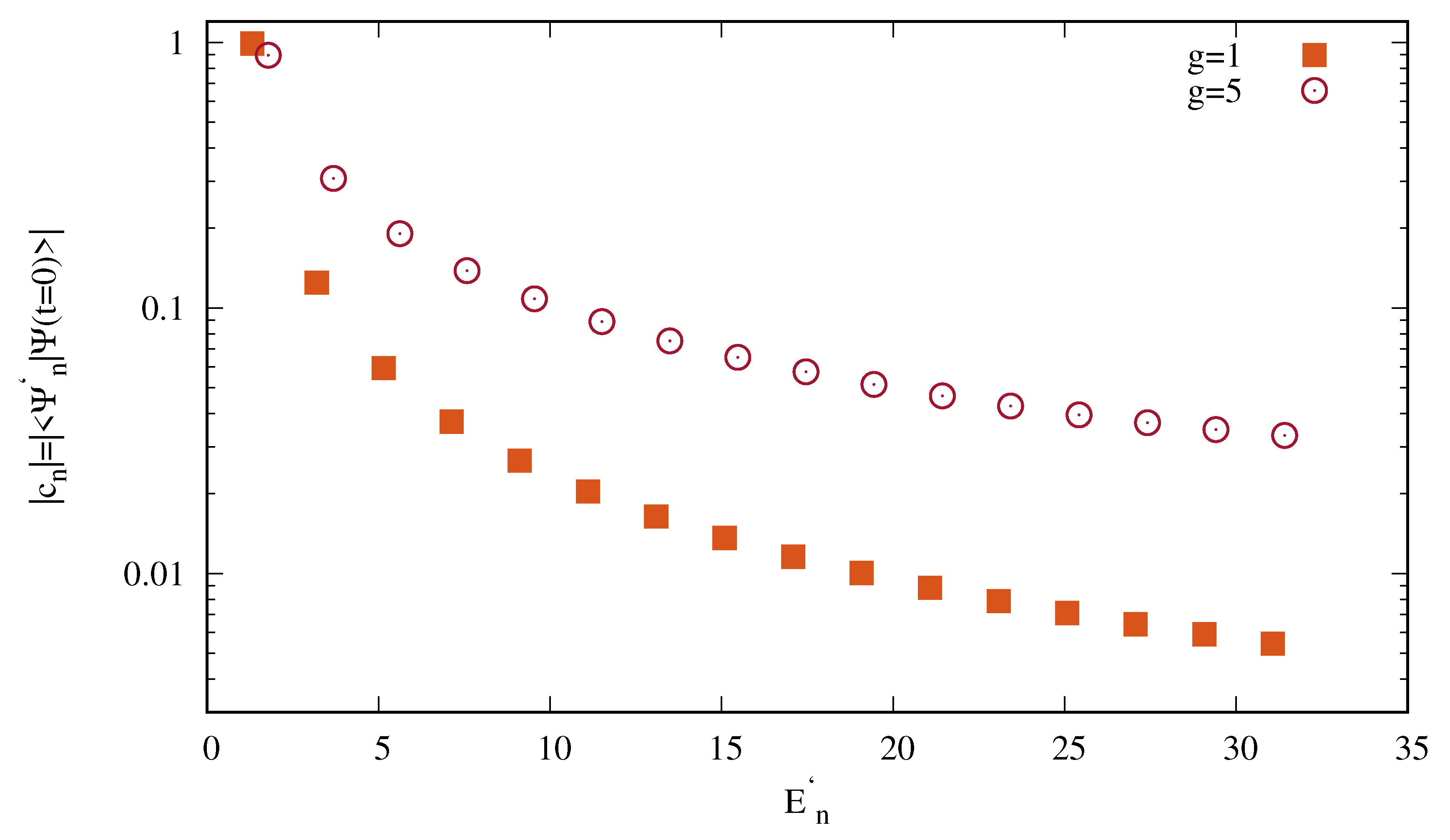
6.2.1. Time Evolution of the Perturbed System

We want to study the time evolution of the ground state corresponding to a given value of g after performing a sudden quench of the interaction strength to a new value $g_{\mathrm{new}}$. The initial ground state is no longer the ground state of the new Hamiltonian. However we can express the old ground state in terms of the eigenvectors of the new Hamiltonian and calculate its time evolution:

$$|\Psi (t=0)\rangle =\sum _n{c}_n|{\Psi }_n^{{}^{\prime }}\rangle ,$$

(61)

where $|\Psi (t=0)\rangle$ is the ground state of the Hamiltonian before the quenching, and the states $|{\Psi }_n^{{}^{\prime }}\rangle$ are the eigenfunctions of the Hamiltonian after the quenching

$$H^{{}^{\prime }}|{\Psi }_n^{{}^{\prime }}\rangle =E_n^{{}^{\prime }}|{\Psi }_n^{{}^{\prime }}\rangle ,$$

(62)

with eigenenergies $E_n^{{}^{\prime }}$. The coefficients $c_n$ can be computed as:

$$c_n=\langle {\Psi }_n^{{}^{\prime }}|\Psi (t=0)\rangle .$$

(63)

The time evolution of the state after the quenching is calculated by taking into account that the states $|{\Psi }_n^{{}^{\prime }}\rangle$ are the eigenstates of the new Hamiltonian,

$$|\Psi \left(t\right)\rangle =\sum _n{c}_n{e}^{-i{E}_n^{{}^{\prime }}t}|{\Psi }_n^{{}^{\prime }}\rangle .$$

(64)

In turn, the eigenstates $|{\psi }_n^{{}^{\prime }}\rangle$ can be expressed in terms of the many-body basis used to describe our system:

$$|{\Psi }_n^{{}^{\prime }}\rangle =\sum _i{C}_{n,i}|{\psi }_i\rangle ,$$

(65)

where $|{\psi }_i\rangle$ is a state of the many-body basis.

Knowing the time evolution of the state we can study the time dependence of any observable. In particular we are going to consider the time evolution of the central density of our system:

$$\rho (x=0,t)=\sum _{i,j}\sum _{k,l}\sum _{n,m}{c}_n^{*}{c}_m{e}^{-i(E_m^{{}^{\prime }}-E_n^{{}^{\prime }})t}{C}_{n,k}^{*}{C}_{m,l}\langle {\psi }_k|a_j^{†}{a}_i|{\psi }_l\rangle {\Phi }_i^{*}\left(0\right){\Phi }_j\left(0\right),$$

(66)

where ${\Phi }_i\left(x\right)$ are the single-particle harmonic oscillator wave functions. Notice that the time evolution of the system is governed by $E_m^{{}^{\prime }}-E_n^{{}^{\prime }}$, involving all energy differences of the states of the new Hamiltonian that have non-zero overlap with the ground-state of the old Hamiltonian. In addition, it is important to realize that the relevance of a given frequency $2\pi {\nu }_{n,m}=E_n-E_m$ depends on the product of the projection coefficients $c_n^{*}{c}_m$.

For instance, it is plausible to think that, for a small change of g, the original ground state should have a large overlap with the new ground state. In this situation the dominant frequencies will be associated to the differences $E_n^{{}^{\prime }}-E_0^{{}^{\prime }}$. In this sense, the frequencies would be similar to the frequencies involved in the calculation of the dynamical structure function associated to the breathing mode of $H^{{}^{\prime }}$, with the exception that the excitations of the center of mass are not present.

In Figure 14, we report, for the two-particle system, the projections of the ground state of the non-interacting system to the eigenstates of $H^{{}^{\prime }}(g=1)$. We also report the projection for the quench $g=0\to 5$. In the case $g=1$ (small g) there is a dominant projection into the ground state of $H^{{}^{\prime }}$ and then the value of the projections decreases rather quickly. For the case $g=5$, the largest projection is smaller than in the previous case but the projections to higher states decrease more slowly. Therefore for $g=5$ one also has relevant projections into higher excited states.

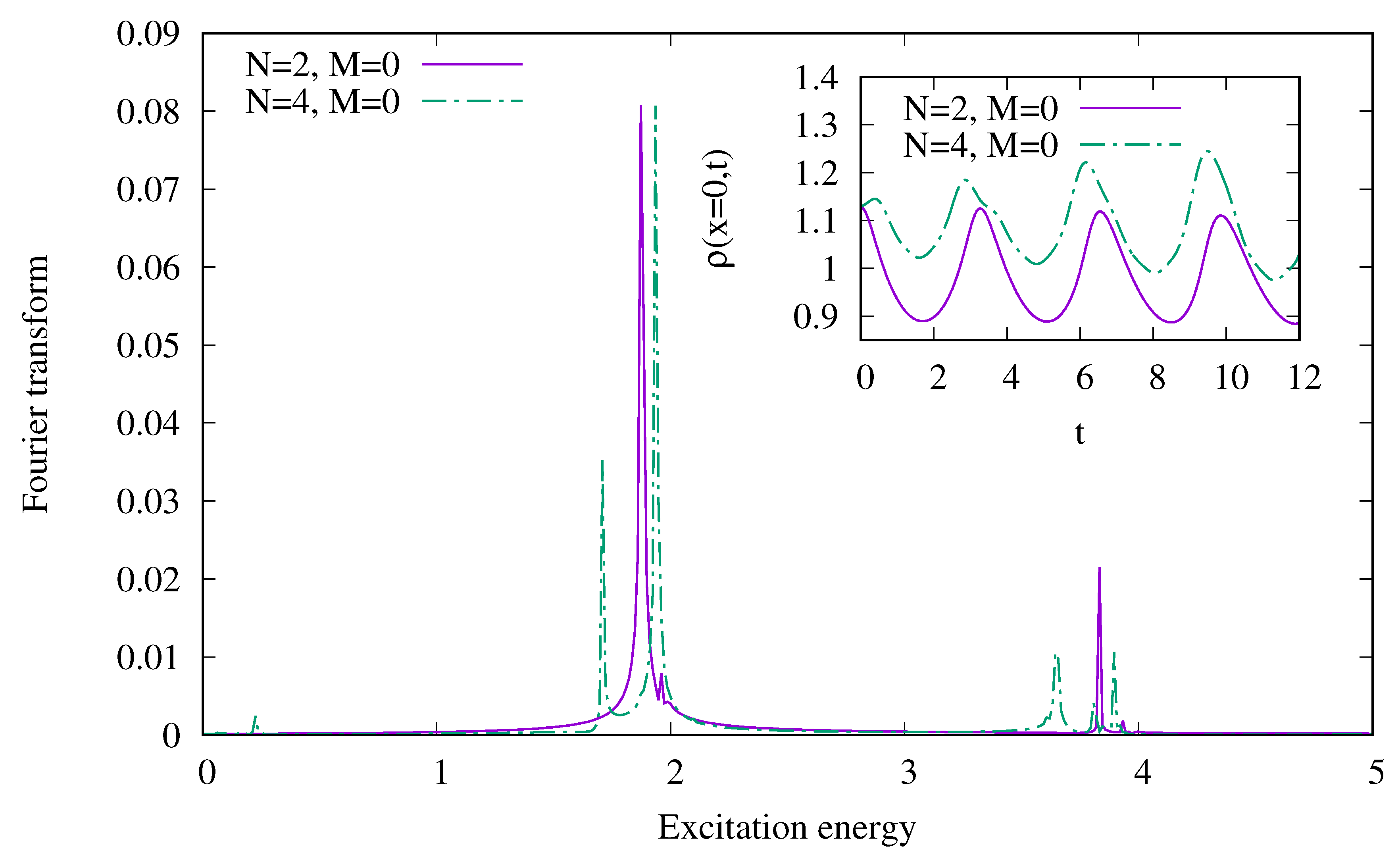
6.2.2. Central Density Oscillations

In this section we propose a method to determine the low energy spectrum of a trapped few-body system, by applying a sudden quench of the strength of the interatomic interactions. In principle, the procedure can be implemented experimentally.

One can prepare a system with N particles trapped in a harmonic potential without interactions. Then apply to the system a sudden quench of the interaction, let the system evolve and measure the central density as a function of time. One should observe an oscillatory behavior.

In order to obtain information about the energy spectrum of the system at $g=1$ (the final value of the quench), we perform a Fourier analysis of the central density as a function of time, see Figure 15. In this way one obtains the characteristic oscillation frequencies which in turn are related to differences of the energies of the system for $g=1$. Therefore, from the frequencies of the Fourier analysis one can reconstruct the excitation energies $\Delta E=2\pi \nu$, mainly with respect to the ground state. To extract the frequencies by Fourier analysis one needs to know the time evolution of the central density in an interval of time much longer than the one shown in the inset of Figure 15. Notice also that it is convenient to subtract the average value of the central density in order to avoid a peak with zero frequency in the Fourier analysis. Actually, this peak at $\nu =0$ does not provide any physical information about the excitation energy spectrum and could overlap with other peaks at low frequencies. We observe a dominant peak at low energy, and more peaks with smaller intensity at higher energies. Although the time interval used to perform the Fourier analysis is very large, the Fourier frequencies still come out with an uncertainty width.

The location of the peaks allows us to recover the excitation energies of the low-excited states with respect to the ground state corresponding to $g=1$. However, to find the absolute energies of these states would be necessary to have access also to the ground-state energy of the system.

The figure reveals the existence of a dominant peak at an excitation energy a little smaller than 2, and other two main visible peaks at energies a little smaller than 4 and 6, with much smaller strength. All these peaks correspond to energy differences of the first excited states, which have non-zero overlap with the non-interacting ground state ($g=0$), and the ground state of the system corresponding to $g=1$, respectively. Notice that the re-entrance phenomenon, discussed in the previous section, is reflected in the fact that the excitation energies are a little smaller than 2, 4, and 6 respectively. It is also worth mentioning the existence of a smaller but distinguishable peak, very close to the excitation energy 2, that corresponds to the difference between the second and first intrinsic excitations (see Figure 8). No center-of-mass excitations affect this analysis.

In the same figure, Figure 15, we present also the case of four particles and spin projection $M=0$. The shape of $\rho (x=0,t)$ shows also an oscillatory behavior, which should be determined by several frequencies. There are two dominant peaks which can be identified, by looking at the excitation spectrum of this system for $g=1$ in Figure 9, with the lowest excitation energies with respect to the ground state. Actually, the small peak that appears at very low energy, corresponds to the energy difference of these two dominant peaks. Notice also that as the ground state has $S=0$, and the interaction is spin independent, the quench cannot connect states with different spins and therefore they do not participate in the time dependence of $\rho (x=0,t)$. As explained for the two-particle case, due to the translation invariance of the interaction, the center-of-mass excitations do not play any role in the analysis. A similar procedure for the time dependence of the mean square radius of the system leads to a determination of the excitation energies consistent with the ones obtained by the analyzing the time dependence of the maximum of the density.

7. Summary and Conclusions

In this paper we have presented a quantum microscopic description of few spin $1/2$ fermions trapped in a 1D harmonic oscillator potential. The fermions interact through a contact interaction that, due to the Pauli principle, is active only between particles with opposite spin. Along the paper, we have mainly concentrated on repulsive interactions. These types of systems have already been realized experimentally and new experiments concerning the structure and mainly the dynamics are expected for the near future. Our main objective has been to study both static and dynamic properties of the system as a function of the interaction strength. This interaction, which provides a good modelization of real interactions, can be experimentally controlled by means of Feshbach resonances.

After a brief introduction, in the second section, we have described the Hamiltonian of the system, that includes both the harmonic oscillator confining potential and the interaction between the fermions. Furthermore, two analytical limits have been discussed in detail: the non-interacting and the infinite interacting limits. In both cases, the many-body wave function, the energy and the density profile of the ground state have been derived. In addition, the second quantization formalism has been introduced as the framework for the calculation of the Hamiltonian.

In the third section we have described in detail the numerical procedures used in the paper, mainly the exact diagonalization techniques. Special attention has been devoted to the convergence problems associated with the dimension of the subspaces of the Hilbert space used to diagonalize the Hamiltonian. The benchmark of the analytical results for the two-particle system has been used to test the accuracy of the numerical methods.

In the next section, we have studied several static properties of the ground state of the system, mainly the total energy and their contributions. The energy contributions have been used to check the fulfillment of the virial relation, obtaining very good results for repulsive interaction, specially in the low-interacting regime. The fulfilment of the virial relation reinforced the consistency of the calculations. We also have discussed the density profile of the ground state. In the non-interacting and the infinite interacting cases our calculations are in perfect agreement with the analytical results presented in the first section. In the next step, we have computed the natural orbits and its eigenvalues. Their analysis reveals the presence of important correlations beyond mean field in the system when the interaction is turned on.

In the last section, we have studied several dynamical properties. First we have studied the response of the system to a mono-polar excitation over the ground state. We have computed the dynamic structure function associated to this perturbation, and using the knowledge of the energy spectra obtained in the previous section, we have identified the excited states. The spin assignment was useful to identify the excited states by the breathing mode. We have also calculated the energy momenta ($M_n$) associated to the dynamic structure function and used the ratios $\sqrt{M_n/M_{n-2}}$ to estimate the average excitation energies. The differences between the ratios $\sqrt{M_n/M_{n-2}}$ for different n indicates the presence of more than one excited state in the dynamic structure function. In fact, for the two particle case there is more than one dominant peak in the response of the system. However, for larger number of particles, even if there are more excited states, the strength of the response is mainly concentrated in one dominant peak.

Finally, we have studied the effect of a quench of the interaction strength on the system. We have discussed the similarities and the differences between the quench and the breathing mode. In addition, we have proposed a possible experimental procedure to measure the excitation energies based on the measurement of the time evolution of the central density of the system after a quench of the interaction. Analyzing the frequencies of the Fourier transform of the time dependence of the oscillation of the central density after the quench one can obtain information about the excitation energies. We expect that the methods and results presented in the paper stimulate the use of exact diagonalization methods to study the dynamics and time evolution of systems with a few fermions in more complicated geometries and different interactions.

References

1. Giamarchi, T. Quantum Physics in One Dimension; Clarendon: Oxford, UK, 2004. [Google Scholar]
2. Tonks, L. The complete equation of state of one, two and three-dimensional gases of hard elastic spheres. Phys. Rev. 1936, 50, 995. [Google Scholar] [CrossRef]
3. Girardeau, M. Relationship between Systems of Impenetrable Bosons and Fermions in One Dimension. J. Math. Phys. 1960, 1, 516. [Google Scholar] [CrossRef]
4. Kinoshita, T.; Wenger, T.; Weiss, D.S. Observation of a one-dimensional Tonks-Girardeau gas. Science 2004, 305, 1125–1128. [Google Scholar] [CrossRef] [PubMed]
5. Paredes, B.; Widera, A.; Murg, V.; Mandel, O.; Fölling, S.; Cirac, I.; Shlyapnikov, G.V.; Hänsch, T.W.; Bloch, I. Tonks—Girardeau gas of ultracold atoms in an optical lattice. Nature 2004, 429, 277–281. [Google Scholar] [CrossRef] [PubMed]
6. Kinoshita, T.; Wenger, T.; Weiss, D.S. Local pair correlations in one-dimensional Bose gases. Phys. Rev. Lett. 2005, 95, 190406. [Google Scholar] [CrossRef] [PubMed]
7. Dalfovo, F.; Giorgini, S.; Pitaevskii, L.P.; Stringari, S. Theory of Bose-Einstein condensation in trapped gases. Rev. Mod. Phys. 1999, 71, 463. [Google Scholar] [CrossRef] [Green Version]
8. Giorgini, S.; Pitaevskii, L.P.; Stringari, S. Theory of ultracold atomic Fermi gases. Rev. Mod. Phys. 2008, 80, 1215. [Google Scholar] [CrossRef] [Green Version]
9. Bloch, I.; Dalibard, J.; Zwerger, W. Many-body physics with ultracold gases. Rev. Mod. Phys. 2008, 80, 885. [Google Scholar] [CrossRef] [Green Version]
10. Lewenstein, M.; Sanpera, A.; Ahufinger, V. Ultracold Atoms in Optical Lattices: Simulating Quantum Many Body Physics; Oxford University Press: Oxford, UK, 2012. [Google Scholar]
11. Serwane, F.; Zürn, G.; Murmann, S.; Brouzos, I.; Lompe, T.; Jochim, S. Deterministic preparation of a tunable few-fermion system. Science 2011, 332, 336–338. [Google Scholar] [CrossRef] [Green Version]
12. Zürn, G.; Serwane, F.; Lompe, T.; Wenz, A.N.; Ries, M.G.; Bohn, J.E.; Jochim, S. Fermionization of two distinguishable fermions. Phys. Rev. Lett. 2012, 108, 075303. [Google Scholar] [CrossRef] [PubMed]
13. Wenz, A.; Zürn, G.; Murmann, S.; Brouzos, I.; Lompe, T.; Jochim, S. From few to many: Observing the formation of a Fermi sea one atom at a time. Science 2013, 342, 457–460. [Google Scholar] [CrossRef] [PubMed] [Green Version]
14. Chin, C.; Grimm, R.; Julienne, P.; Tiesinga, E. Feshbach Resonances in Ultracold Gases. Rev. Mod. Phys. 2010, 82, 1225. [Google Scholar] [CrossRef]
15. Zürn, G.; Wenz, A.N.; Murmann, S.; Bergschneider, A.; Lompe, T.; Jochim, S. Pairing in few-fermion systems with attractive interactions. Phys. Rev. Lett. 2013, 111, 175302. [Google Scholar] [CrossRef] [Green Version]
16. Murmann, S.; Bergschneider, A.; Klinkhamer, V.M.; Zürn, G.; Lompe, T.; Jochim, S. Two fermions in a double well: Exploring a fundamental building block of the Hubbard model. Phys. Rev. Lett. 2015, 114, 080402. [Google Scholar] [CrossRef] [Green Version]
17. Murmann, S.; Deuretzbacher, F.; Zürn, G.; Bjerlin, J.; Reimann, S.M.; Santos, L.; Lompe, T.; Jochim, S. Antiferromagnetic Heisenberg spin chain of a few cold atoms in a one-dimensional trap. Phys. Rev. Lett. 2015, 115, 215301. [Google Scholar] [CrossRef] [PubMed]
18. Hammer, H.-W.; Nogga, A.; Schwenk, A. Three-body forces: From cold atoms to nuclei. Rev. Mod. Phys. 2013, 85, 197. [Google Scholar] [CrossRef] [Green Version]
19. Ring, P.; Schuck, P. The Nuclear Many-Body Problem; Springer: Berlin/Heidelberg, Germany, 1980. [Google Scholar]
20. Truscott, A.G.; Strecker, K.E.; McAlexander, W.I.; Partridge, G.B.; Hulet, R.G. Observation of Fermi Pressure in a Gas of Trapped Atoms. Science 2001, 291, 2570. [Google Scholar] [CrossRef] [Green Version]
21. Blume, D. Few-body physics with ultracold atomic and molecular systems in traps. Rep. Prog. Phys. 2012, 75, 046401. [Google Scholar] [CrossRef] [Green Version]
22. Mistakidis, S.I.; Katsimiga, G.C.; Koutentakis, G.M.; Schmelcher, P. Repulsive Fermi polarons and their induced interactions in binary mixtures of ultracold atoms. New J. Phys. 2019, 21, 043032. [Google Scholar] [CrossRef] [Green Version]
23. Zöllner, S.; Meyer, H.-D.; Schmelcher, P. Correlations in ultracold trapped few-boson systems: Transition from condensation to fermionization. Phys. Rev. A 2006, 74, 063611. [Google Scholar] [CrossRef] [Green Version]
24. Cheiney, P.; Cabrera, C.R.; Sanz, J.; Naylor, B.; Tanzi, L.; Tarruell, L. Bright Soliton to Quantum Droplet Transition in a Mixture of Bose-Einstein Condensates. Phys. Rev. Lett. 2018, 120, 135301. [Google Scholar] [CrossRef] [PubMed] [Green Version]
25. Sowinski, T.; Garcia-March, M.A. One-dimensional mixtures of several ultracold atoms: A review. Rep. Prog. Phys. 2019, 82, 104401. [Google Scholar] [CrossRef] [Green Version]
26. Laird, E.K.; Shi, Z.-Y.; Parish, M.M.; Levinsen, J. SU(N) fermions in a one-dimensional harmonic trap. Phys. Rev. A 2017, 96, 032701. [Google Scholar] [CrossRef] [Green Version]
27. Brouzos, I.; Schmelcher, P. Two-component few-fermion mixtures in a one-dimensional trap: Numerical versus analytical approach. Phys. Rev. A 2013, 87, 023605. [Google Scholar] [CrossRef] [Green Version]
28. Lindgren, E.J.; Rotureau, J.; Forssén, C.; Volosniev, A.G.; Zinner, N.T. Fermionization of two-component few-fermion systems in a one-dimensional harmonic trap. New J. Phys. 2014, 16, 063003. [Google Scholar] [CrossRef] [Green Version]
29. Andersen, M.E.S.; Dehkharghani, A.S.; Volosniev, A.G.; Lindgren, E.J.; Zinner, N.T. An interpolatory ansatz captures the physics of one-dimensional confined Fermi systems. Sci. Rep. 2016, 6, 28362. [Google Scholar] [CrossRef] [PubMed] [Green Version]
30. Pęcak, D.; Dehkharghani, A.S.; Zinner, N.T.; Sowiński, T. Four fermions in a one-dimensional harmonic trap: Accuracy of a variational-ansatz approach. Phys. Rev. A 2017, 95, 053632. [Google Scholar] [CrossRef] [Green Version]
31. Gordillo, M.C. One-dimensional harmonically confined SU(N) fermions. Phys. Rev. A 2019, 100, 023603. [Google Scholar] [CrossRef] [Green Version]
32. Harshman, N.L. Spectroscopy for a few atoms harmonically trapped in one dimension. Phys. Rev. A 2014, 89, 033633. [Google Scholar] [CrossRef] [Green Version]
33. Sowinski, T.; Grass, T.; Dutta, O.; Lewenstein, M. Few interacting fermions in one-dimensional harmonic trap. Phys. Rev. A 2013, 88, 033607. [Google Scholar] [CrossRef] [Green Version]
34. Ledesma, D.; Romero-Ros, A.; Polls, A.; Juliá-Díaz, B. Dynamic structure function of two interacting atoms in 1D. EPL 2019, 127, 56001. [Google Scholar] [CrossRef]
35. Pyzh, M.; Kronke, S.; Weitenberg, C.; Schmelcher, P. Spectral properties and breathing dynamics of a few-body Bose-Bose mixture in a 1D harmonic trap. New J. Phys. 2018, 20, 015006. [Google Scholar] [CrossRef]
36. Olshanii, M. Atomic scattering in the presence of an external confinement and a gas of impenetrable bosons. Phys. Rev. Lett. 1998, 81, 938. [Google Scholar] [CrossRef] [Green Version]
37. Haller, E.; Gustavsson, M.; Mark, M.J.; Danzl, J.G.; Hart, R.; Pupillo, G.; Nagerl, H.-C. Realization of an Excited, Strongly Correlated Quantum Gas Phase. Science 2009, 325, 1224. [Google Scholar] [CrossRef] [PubMed] [Green Version]
38. Yin, X.Y.; Yan, Y.; Smith, D.H. Dynamics of small trapped one-dimensional Fermi gas under oscillating magnetic fields. Phys. Rev. A 2016, 94, 043639. [Google Scholar] [CrossRef] [Green Version]
39. Guan, L.; Chen, S.; Wang, Y.; Ma, Z. Exact solution for infinitely strongly interacting Fermi gases in tight waveguides. Phys. Rev. Lett. 2009, 102, 160402. [Google Scholar] [CrossRef] [Green Version]
40. Volosniev, A.G.; Fedorov, D.V.; Jensen, A.S.; Valiente, M.; Zinner, N.T. Strongly interacting confined quantum systems in one dimension. Nat. Commun. 2014, 5, 5300. [Google Scholar] [CrossRef] [Green Version]
41. Lieb, E.H.; Mattis, D. Theory of ferromagnetism and the ordering of electronic energy levels. Phys. Rev. 1962, 125, 164. [Google Scholar] [CrossRef]
42. Decamp, J.; Armagnat, P.; Fang, B.; Albert, M.; Minguzzi, A.; Vignolo, P. Exact density profiles and symmetry classification for strongly interacting multi-component Fermi gases in tight waveguides. New J. Phys. 2016, 18, 055011. [Google Scholar] [CrossRef]
43. Dickhoff, W.H.; van Neck, D. Many-Body Theory Exposed! World Scientific: Singapore, 2008. [Google Scholar]
44. Busch, T.; Englert, B.G.; Rzazewski, K.; Wilkens, M. Two cold atoms in an harmonic trap. Found. Phys. 1998, 28, 549. [Google Scholar] [CrossRef]
45. Wu, K.; Simon, H. Thick-restart Lanczos method for large symmetric eigenvalue problems. SIAM J. Matrix Anal. Appl. 2000, 22, 602. [Google Scholar] [CrossRef]
46. Meyer, H.D.; Manthe, U.; Cederbaum, L.S. The multi-configurational time-dependent Hartree approach. Chem. Phys. Lett. 1990, 165, 73. [Google Scholar] [CrossRef]
47. Rammelmüller, L.; Porter, W.J.; Braun, J.; Drut, J. Evolution from few- to many-body physics in one-dimensional Fermi systems: One- and two-body density matrices and particle-partition entanglement. Phys. Rev. A 2017, 96, 033635. [Google Scholar] [CrossRef] [Green Version]
48. Bellotti, F.F.; Dehkharghani, A.S.; Zinner, N.T. Comparing numerical and analytical approaches to strongly interacting two-component mixtures in one dimensional traps. Eur. Phys. J. D 2017, 71, 37. [Google Scholar] [CrossRef] [Green Version]
49. Raventos, D.; Grass, T.; Lewenstein, M.; Juliá-Díaz, B. Cold bosons in optical lattices: A tutorial for Exact Diagonalization. J. Phys. B At. Mol. Opt. Phys. 2017, 50, 113001. [Google Scholar] [CrossRef] [Green Version]
50. Plodzien, M.; Wiater, D.; Chrostowski, A.; Sowinski, T. Numerically exact approach to few-body problems far from a perturbative regime. arXiv 2018, arXiv:1803.08387. [Google Scholar]
51. Chrostowski, A.; Sowiński, T. Efficient construction of many-body Fock states having the lowest energies. Acta Phys. Pol. A 2020, 136, 566. [Google Scholar] [CrossRef]
52. Titchmarsh, E.C. Some integral Involving Hermite Polynomials. J. Lond. Math. Soc. 1948, 23, 15. [Google Scholar] [CrossRef]
53. Grining, T.; Tomza, M.; Lesiuk, M.; Przybytek, M.; Musial, M.; Massignan, P.; Lewenstein, M.; Moszynski, R. Many interacting fermions in a one-dimensional harmonic trap: A quantum-chemical treatment. New J. Phys. 2015, 17, 115001. [Google Scholar] [CrossRef]
54. Gharashi, S.E.; Blume, D. Correlations of the upper branch of 1d harmonically trapped two-component Fermi gases. Phys. Rev. Lett. 2013, 111, 045302. [Google Scholar] [CrossRef]
55. Li, X.; Pecak, D.; Sowinski, T.; Sherson, J.; Nielsen, A.E.B. Global optimization for quantum dynamics of few-fermion systems. Phys. Rev. A 2018, 97, 033602. [Google Scholar] [CrossRef] [Green Version]
56. Fang, B.; Carleo, G.; Bouchoule, I. Quench-induced breathing mode of one-dimensional Bose gases. Phys. Rev. Lett. 2014, 113, 035301. [Google Scholar] [CrossRef] [PubMed] [Green Version]
57. Menotti, C.; Stringari, S. Collective oscillations of a 1D trapped Bose gas. Phys. Rev. A 2002, 66, 043610. [Google Scholar] [CrossRef] [Green Version]
58. Moritz, H.; Stoferle, T.; Kohl, M.; Esslinger, T. Exciting Collective Oscillations in a Trapped 1D Gas. Phys. Rev. Lett. 2003, 91, 250402. [Google Scholar] [CrossRef] [PubMed] [Green Version]
59. Kohn, W. Cyclotron Resonance and de Haas-van Alphen Oscillations of an Interacting Electron Gas. Phys. Rev. 1961, 123, 1242. [Google Scholar] [CrossRef]
60. Ebert, M.; Volosniev, A.; Hammer, H.-W. Two Cold Atoms in a Time-Dependent Harmonic Trap in One Dimension. Ann. Phys. 2016, 528, 698. [Google Scholar] [CrossRef] [Green Version]
61. Gharashi, S.E.; Blume, D. Broken scale-invariance in time-dependent trapping potentials. Phys. Rev. A 2016, 94, 063639. [Google Scholar] [CrossRef] [Green Version]
62. Kwasniok, J.; Mistakidis, S.I.; Schmelcher, P. Correlated dynamics of fermionic impurities induced by the counterflow of an ensemble of fermions. Phys. Rev. A 2020, 101, 053619. [Google Scholar] [CrossRef]
63. Gudyma, A.I.; Astrakharchik, G.E.; Zvonarev, M.B. Reentrant behavior of the breathing-mode-oscillation frequency in a one-dimensional. Phys. Rev. A 2015, 92, 021601. [Google Scholar] [CrossRef] [Green Version]
64. Bohigas, O.; Lane, A.M.; Martorell, J. Sum rules for nuclear collective excitations. Phys. Rep. 1979, 51, 267. [Google Scholar] [CrossRef]
65. Sowinski, T.; Brewczyk, M.; Gajda, M.; Rzazewski, K. Exact dynamics and decoherence of two cold bosons in a 1D harmonic trap. Phys. Rev. A 2010, 82, 053631. [Google Scholar] [CrossRef] [Green Version]
66. Budewig, L.; Mistakidis, S.I.; Schmelcher, P. Quench Dynamics of Two One-Dimensional Harmonically Trapped Bosons Bridging Attraction and Repulsion. Mol. Phys. 2019, 117, 2043. [Google Scholar] [CrossRef] [Green Version]
67. Erdmann, J.; Mistakidis, S.I.; Schmelcher, P. Phase-separation dynamics induced by an interaction quench of a correlated Fermi-Fermi mixture in a double well. Phys. Rev. A 2019, 99, 013605. [Google Scholar] [CrossRef] [Green Version]
Figure 1. Energy spectrum of the two-particle system as a function of the interaction strength. The calculations are performed using 100 single-particle modes (green dots). The analytical spectrum (dashed red line) is obtained with Equation (43) for the energy of the relative system and adding after the possible energies of the center of mass. Energy given in harmonic oscillator units. The energies obtained via Equation (43) correspond to even-parity states, the corresponding odd-parity states do not depend on the interaction, and result in horizontal lines in close agreement with the numerical ones.
Mathematics 08 01196 g001
Figure 2. Differences between the numerical results and the exact ones as a function of the number of single particle modes, for two values of the interaction strength, g = 1 and g = 5 , for the ground (g.s) and first excited (ex.) state. The lines are fits of the type C 1 / N M 1 / 2 + C 2 / N M to the calculated points. Both axes are in a logarithmic scale.
Mathematics 08 01196 g002
Figure 3. Ground-state energy as a function of the interaction strength for different number of particles and spin configurations. The calculations have been performed by using 100, 50, 40 and 30 single-particle modes to construct the many-body basis for N = 2,3,4 and 5 particles respectively. The black squares are the corresponding results reported in Ref. [54].
Mathematics 08 01196 g003
Figure 4. Different energy contributions to the total ground-state energy, as a function of the interaction strength for different number of particles and total third-spin component. The total energy and the fulfilment of the virial theorem is also shown (Equation (47)). The legend is common to all graphics.
Mathematics 08 01196 g004
Figure 5. Density profiles of the ground state for different number of particles and spin projections. The density profiles are shown for various values of the interaction strength. The legend is common to all panels.
Mathematics 08 01196 g005
Figure 6. Densities of the spin up ( ρ , left panels) and spin down ( ρ , right panels) particles in the ground state. The density profiles are shown for various values of the interaction strength and for different number of particles and spin projection. The legend is common to all panels. The corresponding total densities are reported in Figure 5.
Mathematics 08 01196 g006
Figure 7. The largest 10 eigenvalues of the one-body density matrix (OBDM) of the ground state of systems with different number of particles and spin configurations as a function of the interaction strength.
Mathematics 08 01196 g007
Figure 8. Low-energy spectrum for several number of particles and spin configurations as a function of the interaction strength. Notice that the excitation energies are measured with respect to the ground-state energy of the non-interacting system.
Mathematics 08 01196 g008
Figure 9. Low-energy spectrum of the fermionic system with four particles as a function of the interaction strength. The states are labelled according to their total spin, as explained in the text.
Mathematics 08 01196 g009
Figure 10. Dynamic structure function of a mono-polar excitation for the case of two fermions. The total spin of the ground state and of all excited states connected to it through the mono-polar excitation, are zero. The different panels correspond to four different values of interaction strength. From the non-interacting case, g = 0 to a strongly interacting one g = 15 .
Mathematics 08 01196 g010
Figure 11. Dynamic structure function of a mono-polar excitation for the case of four particles. The total spin of the ground state and of all excited states connected to it through the mono-polar excitation, are zero. The different panels correspond to four different values of interaction strength. From the non-interacting case, g = 0 to a strongly interacting one g = 15 .
Mathematics 08 01196 g011
Figure 12. Values of the three energy momenta M 1 , M 1 and M 3 for the cases of two and four particles as a function of the interaction strength. The calculations done using the explicit value of the dynamic structure function, Equation (57) are represented by dots and the line is the value computed using the sum rules, Equation (59). For M 1 the results from Equations (59) and (60) are indistinguishable on the figure.
Mathematics 08 01196 g012
Figure 13. Ratios of the sum rules M 1 / M 1 and M 3 / M 1 as a function of the interaction strength for several number of particles and spin configurations. The purple + signs correspond to the excitation energy of the main peak of the dynamic structure function.
Mathematics 08 01196 g013
Figure 14. Projection of the initial ground state for g = 0 into the eigenstates of g = 1 and g = 5 as a function of its energy, for a two particles systems with zero total spin. The y axis is in logarithmic scale.
Mathematics 08 01196 g014
Figure 15. Frequency analysis of the time dependence of the central density after an interaction quench from g = 0 to g = 1 . The average density has been subtracted. We consider the cases N = 2 (solid lines) and N = 4 (dot-dashed lines). In the inset we depict the first oscillations of the signal used to compute the Fourier analysis shown in the main panels. For the Fourier analysis we used a time interval, t = 500. All magnitudes in the figure are in harmonic oscillator units.
Mathematics 08 01196 g015