Fractional Order PID Controller Design for an AVR System Using Chaotic Yellow Saddle Goatfish Algorithm

Abstract

This paper presents a novel method for optimal tunning of a Fractional Order Proportional-Integral-Derivative (FOPID) controller for an Automatic Voltage Regulator (AVR) system. The presented method is based on the Yellow Saddle Goatfish Algorithm (YSGA), which is improved with Chaotic Logistic Maps. Additionally, a novel objective function for the optimization of the FOPID parameters is proposed. The performance of the obtained FOPID controller is verified by comparison with various FOPID controllers tuned by other metaheuristic algorithms. A comparative analysis is performed in terms of step response, frequency response, root locus, robustness test, and disturbance rejection ability. Results of the simulations undoubtedly show that the FOPID controller tuned with the proposed Chaotic Yellow Saddle Goatfish Algorithm (C-YSGA) outperforms FOPID controllers tuned by other algorithms, in all of the previously mentioned performance tests.

1. Introduction

The quality of electrical energy is the main demand from consumers in the power system. Since the indicators of the quality are voltage and frequency, these parameters must be maintained at the desired level at every moment. Generally, in every power system, the frequency depends on the active power flow, while the reactive power flow has a greater impact on the voltage level. Additionally, any deviation of the voltage from the nominal value requires the flow of the reactive power, which automatically increases line losses. The fluctuations of the voltage can be repressed using various devices: serial and parallel capacitor banks, synchronous compensators, tap-changing transformers, reactors, Static VAr Compensators (SVC), and Automatic Voltage Regulators (AVR) [1,2]. This paper deals with AVR systems.

The AVR represents the main control loop for the voltage regulation of the synchronous generator (SG), which is the main unit for producing electrical energy in the whole power system. Concretely, the control of the terminal voltage of the synchronous generator is achieved by adjusting its’ exciter voltage. Although the main task of the AVR is to provide stable voltage level at the generator’s terminals, it is also very important in improving the dynamic response of the terminal voltage. Regardless of the fact that the control theory developed many modern control techniques, the traditional PID controller is still the most used in the AVR systems. In general, in this paper, the optimal tuning of the controller is considered.

Enhancing the performance of the PID controller for AVR systems is possible by using fractional calculus. Fractional order PID controller (FOPID) is the general form of the PID controller that uses fractional order of derivatives and integrals, instead of integer order. Moreover, FOPID can provide a better transient response and is more robust and stable compared to the conventional (known as integer order controller) PID controller [3]. Due to the previously mentioned advantages of the FOPID, this paper deals with this type of controller.

The optimal design of the FOPID controller implies determining the parameters to satisfy defined optimization criteria (or fitness/objective function). In the available literature, the most used method for optimal tuning of the FOPID controller is based on metaheuristic algorithms [4,5,6,7,8,9,10,11,12]. Particle Swarm Optimization (PSO) and Genetic Algorithm (GA) are applied in [4,5,8,11] to determine the optimal values of the FOPID parameters. For the same purpose, D. L. Zhang et al. proposed an Improved Artificial Bee Colony Algorithm (CNC-ABC) [6]. Also, it can be found that the authors used Chaotic Ant Swarm (CAS) [7], Multi-Objective Extremal Optimization (MOEO) [9], Cuckoo Search (CS) [10], and Salp Swarm Optimization (SSO) algorithm [12] to determine unknown parameters of the FOPID. Besides the FOPID, many existing studies deal with the optimization of the parameters of the classical PID controller for the AVR systems [13,14,15,16,17,18,19,20,21,22].

Another very important aspect of the optimization process that needs to be particularly reviewed is the choice of the fitness function. Previously mentioned algorithms introduce a huge variety of fitness functions that take into account time-domain (rise time, settling time, overshoot, and steady-state error), as well as frequency domain parameters (gain margin, phase margin, gain crossover frequency, and so on). One of the most common error-based functions is Integrated Absolute Error (IAE) [6]. Another commonly used time-domain criterion is Zwee Lee Gaing’s function originally proposed in [13] for PID controller tuning and applied in [7,10] for optimal tunning of the FOPID controller. Ortiz-Quisbert et al. used the complex function that tends to minimize only time-domain parameters: overshoot, settling time, and maximum voltage signal derivative [11]. One of the most interesting approaches in a fitness function definition is combining error-based functions with time-domain parameters, as presented in [8,9,11]. Concretely, an interesting approach minimizes the Integrated Time Squared Error (ITSE) of the output voltage, energy of the control signal, and ITSE of the load disturbance [8]. The objective function in [9] is composed of IAE, steady-state error, and settling time, while in [11], the objective is to minimize not only IAE, steady-state error, and settling time as previously mentioned, but also the overshoot and the control signal energy. Fitness function that consists only of the frequency domain parameters is proposed in [5] and tends to maximize phase margin and the gain crossover frequency. The trade-off between different frequency domain parameters (phase margin and gain margin) and time-domain parameters (overshoot, rise time, settling time, steady-state error, IAE, and control signal energy) is formulated as an objective function in [4].

Although a large number of FOPID tuning techniques have been proposed in the available literature, the optimal design of the FOPID controller can still be improved by further research. To that end, this paper proposes a novel design approach of the FOPID controller. The contributions of this work are highlighted as follows:

• Firstly, the recently proposed Yellow Saddle Goatfish Algorithm (YSGA) [23] is merged with Chaos Optimization Algorithm [24] in order to obtain novel Chaotic Yellow Saddle Goatfish Algorithm (C-YSGA). Original YSGA can improve the optimization process in terms of accuracy and convergence in comparison to several state-of-the-art optimization methods. The improvement is proven by applying this method on five engineering problems, while the comparison with other methods is carried out by using 27 well-known functions [23]. Additionally, in this paper, the superiority of the original YSGA over several other metaheuristic techniques will be demonstrated on the particular optimization problem. Moreover, an improvement of the YSGA by adding Chaotic Logistic Mapping is introduced. The purpose of merging two algorithms is to additionally improve the convergence speed of the YSGA algorithm. Therefore, the original optimization algorithm for optimal tuning of the FOPID controller will be presented in this paper.
• Afterward, the new objective function that tends to optimize time-domain parameters has been proposed. It is demonstrated that the usage of the proposed objective function provides significantly better results than the other functions proposed in the literature.
• Such an obtained FOPID controller has been compared with those tuned by different optimization algorithms in terms of transient response quality. The conducted analysis clearly demonstrates the superiority of the FOPID controller tuned by C-YSGA.
• Finally, different uncertainties have been introduced to the system in order to examine its behavior. Precisely, the robustness test that implies changing the AVR system parameters is carried out. Also, the ability of the system to cope with the different disturbances (control signal disturbance, load disturbance, and measurement noise) is investigated. During all of the mentioned tests, the FOPID controller tuned by C-YSGA shows significantly better performances compared to the FOPID controller, whose parameters are optimized by the other algorithms considered in the literature.

The organization of this paper is as follows. A brief overview of the AVR system, along with the performance analysis, is provided in Section 2. Section 3 demonstrates the basics of the fractional-order calculus, which is needed for simulating a FOPID controller. Afterward, a compact and wide overview of the available literature related to FOPID parameters optimization is given in Section 4. Section 5 shows the mathematical formulation of the novel C-YSGA algorithm that is presented in this paper. The results of the simulation are given in Section 6. Conclusions are provided in Section 7.

2. Description of the AVR System

The primary function of an AVR system is to maintain the terminal voltage of the generator at a constant level through the excitation system. However, due to the different disturbances in the power system, a synchronous generator does not always work at the equilibrium point. Such oscillations around the equilibrium state can cause deviations of the frequency and the voltage, which can be very harmful to the overall stability of the power system. In order to enhance the dynamic stability of the power system, as well as to provide quality energy to the consumers, excitation systems equipped with AVR are employed. Because of such an important role, the design of an AVR system is a crucial and challenging task.

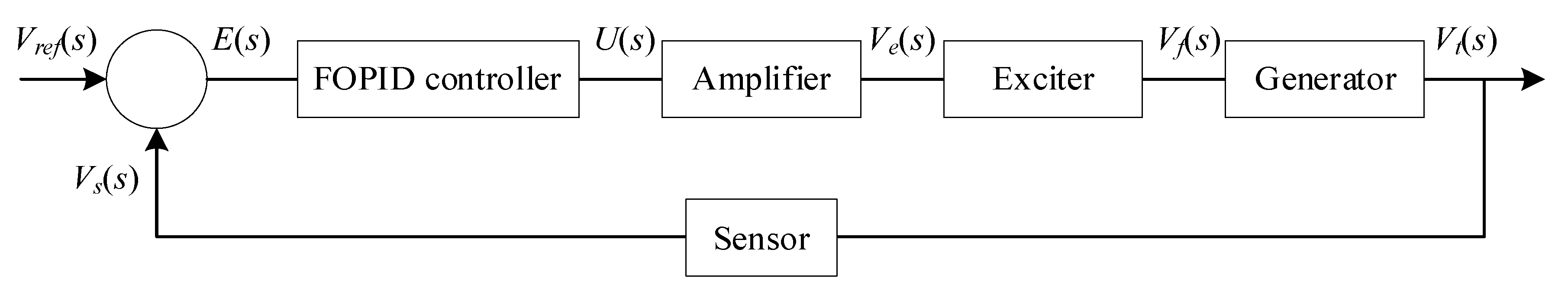
A typical AVR system consists of the following components:

• controller,
• amplifier,
• exciter,
• generator, and
• sensor.

The object that needs to be controlled in this control scheme is a synchronous generator, whose terminal voltage is measured and rectified by the sensor. An error signal, which presents the difference between the desired and the measured voltage value, is formed in the comparator. One of the main components in the AVR scheme that needs to be chosen carefully is the controller. Based on the error signal and the appropriate control algorithm selected, the controller defines the control signal. Very often the controller is realized as a microcontroller unit, whose output power is deficient. Due to this, the existence of the amplifier is necessary in order to increase the power of the control signal. Finally, an amplified signal is used to control the excitation system of the synchronous generator, and therefore, to define the terminal voltage level. The scheme of such a described system is depicted in Figure 1.

In the available literature [4,5,6,7,8,9,10,11,12,13,14,15,16,17,18,19,20,21,22], the components of the AVR (except the controller) are presented as the first-order transfer function, which is composed of gain and time constant.

Table 1. Transfer functions of each AVR system component.

Component	Transfer Function	Range of the Parameters
Amplifier	KA/(1 + sTA)	10 ≤ KA ≤ 400, 0.02 s ≤ TA ≤ 0.1 s
Exciter	KE/(1 + sTE)	1 ≤ KE ≤ 10, 0.4 s ≤ TE ≤ 1 s
Generator	KG/(1 + sTG)	0.7 ≤ KG ≤ 1, 1 s ≤ TG ≤ 2 s
Sensor	KS/(1 + sTS)	1 ≤ KS ≤ 2, 0.001 s ≤ TS ≤ 0.06 s

gives a compact review of the transfer functions and the range of each parameter.

In the previous table, K_A, K_E, K_G, and K_S stand for gains of an amplifier, exciter, generator, and sensor, respectively, while T_A, T_E, T_G, and T_S are time constants of the amplifier, exciter, generator, and sensor. Values that are considered in this paper are K_A = 10, K_E = 1, K_G = 1, K_S = 1, T_A = 0.1, T_E = 0.4, T_G = 1, and T_S = 0.01 [5,6,7,8,9,10,11,12,13,14,15,16,17,18,19,20,21,22]. It is important to mention that the gain of the generator K_G depends on the load of the generator. Namely, K_G can take a value from 0.7 (non-loaded generator) to 1 (nominal loaded generator).

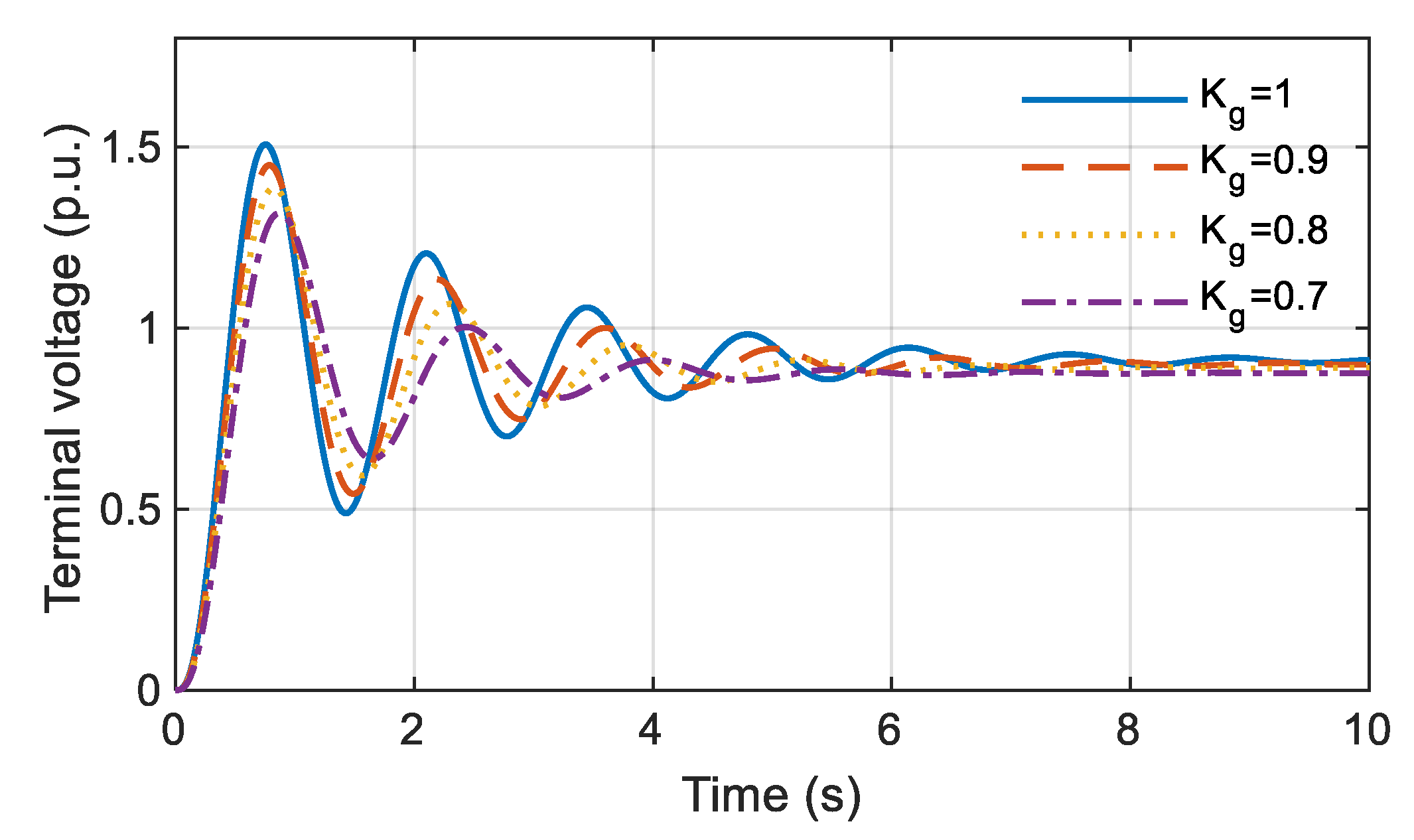
Before including the controller in the system analysis, it is necessary to carry out the analysis of the system in the absence of the controller. To that end, the step response of the AVR system without the controller is given in Figure 2. In order to demonstrate the behavior of the system in the different cases of the load, simulations are conducted for different values of parameter K_G (0.7, 0.8, 0.9, and 1).

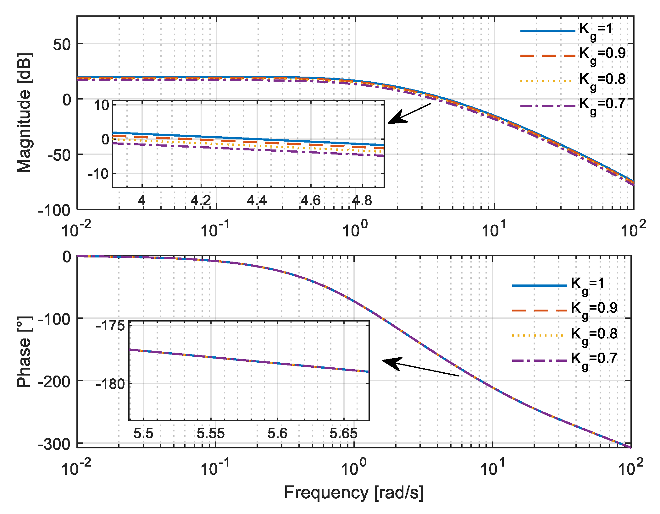
Despite the transient response (time-domain) analysis, it is also very important to take a look at the frequency response of the system. Frequency characteristics or Bode diagrams of the open-loop system can provide information about margins of the stability of the closed-loop system. Precisely, it is important to determine the values of the gain margin and the phase margin, which both need to be positive in order to have a stable system. For the different values of the parameter K_G, frequency responses are shown in Figure 3.

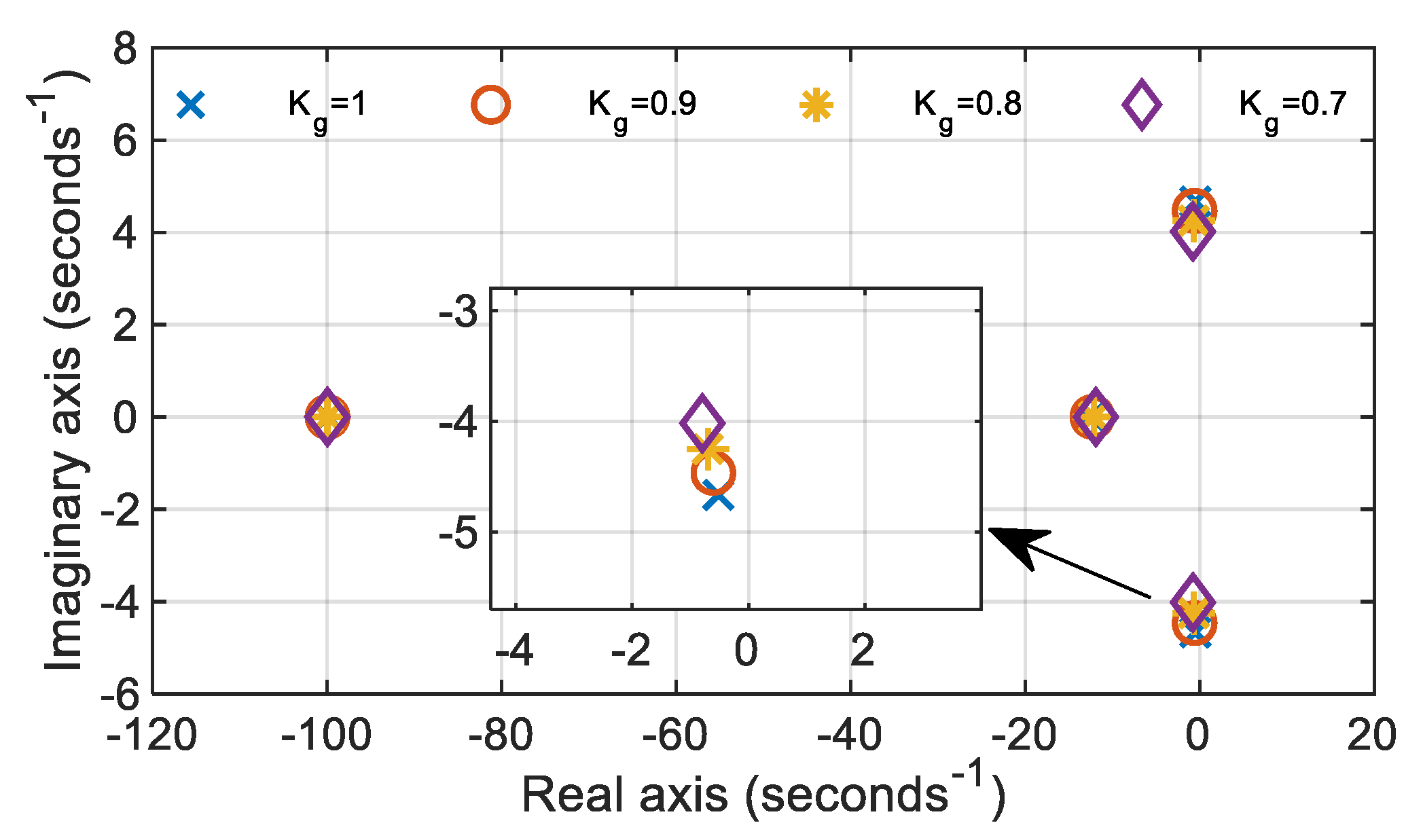
Another essential characteristic of the system, and the main indicator of stability, is the root locus of the closed-loop system. Root locus gives information about the location of the poles of the closed-loop system. As it is well known from control theory, for the stable system, all the poles must be located in the left half-plane. The graphical representation of the location of the poles is given in Figure 4.

Based on the previously presented figures, all-important time domain and frequency domain parameters can be computed. Namely,

Table 2. Values of the transient response and frequency response parameters.

Parameter	KG = 1	KG = 0.9	KG = 0.8	KG = 0.7
Overshoot (%)	65.214	61.3825	55.9051	50.4818
Rise time (s)	0.2613	0.2755	0.2945	0.3171
Settling time (s)	7.0192	6.5237	5.4086	4.9012
Steady-state error (p.u.)	0.0881	0.102	0.1108	0.1249
Closed-loop system poles	−0.51 ± 4.66i −12.48 −99.97	−0.6 ± 4.46i −12.31 −99.97	−0.69 ± 4.25i −12.12 −99.97	−0.79 ± 4.01i −11.92 −99.97
Gain margin (dB)	4.61	5.53	6.55	7.71
Phase margin (o)	16.1	19.56	23.56	28.26

shows transient response indices-rise time (t_r), settling time (t_s), overshoot in percentage (OS), steady-state error (E_ss), frequency response parameters-gain margin (G_m) and phase margin (P_m), as well as the poles of the closed-loop system.

Root locus and frequency characteristics prove that the AVR system is stable, but the margins of the stability are low due to the poles that are very close to the imaginary axis of the complex plane. Also, large values of the overshoot, the settling time, and the steady-state error indicate that the transient response of the AVR system in the absence of the controller is feeble. In fact, the steady-state error varies from 8% to 12% (depending on the load of the generator), which means the AVR cannot complete the main task—maintaining the voltage level at the reference value. All of the aforementioned deficiencies can be eliminated by adding the controller into the system. According to the available literature, the most used control strategies for AVR systems are based on classical or integer-order PID controller, as well as the generic version of the PID controller that is called Fractional-Order PID controller (FOPID).

Integer-order PID controller is presented by the following transfer function:

$$PID\left(s\right)=K_p+\frac{K_i}{s}+K_{d}s,$$

(1)

where K_p is the proportional gain, K_i is the integral gain, and K_d is the derivative gain. Integer-order is a specific case of the PID controller, where the integral and the derivative are first order.

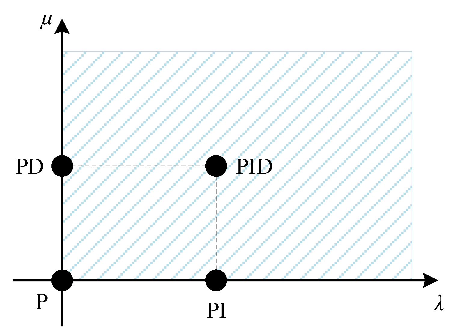
The general type of the PID controller is called Fractional-Order PID controller and is presented using the following transfer function:

$$FOPID\left(s\right)=K_p+\frac{K_i}{s^{\lambda }}+K_d{s}^{\mu },$$

(2)

where λ and μ represent the order of the integral and of the derivative, respectively. As the name of the FOPID indicates, these two numbers can be any real numbers (not strictly integers). The aforementioned facts make the FOPID the most general form of the PID controller. Specific forms of FOPID controllers are PID (λ = 1, μ = 1), PI (λ = 1, μ = 0), PD (λ = 0, μ = 1) and P controller (λ = 0, μ = 0), as illustrated in Figure 5.

3. About the Fractional Order Calculus

Regarding the problem of the fractional-order calculus, many different approaches have been proposed. According to [3], the most commonly used definitions of the fractional-order calculus are Grunwald–Letnikov, Riemann–Liouville, and Caputo definition.

Grundwald–Letnikov’s approach defines the αth order derivative of the function f in the limits from a to t as follows:

$$D^{\alpha }\underset{a}{\overset{t}{|}}=\underset{h\to 0}{\lim }\frac{1}{h^{\alpha }}{\displaystyle \sum _{r=0}^{\left[\frac{t-a}{h}\right]}{\left(-1\right)}^r}\left(\begin{array}{c}n\\ r\end{array}\right)f(t-rh),$$

(3)

where h stands for the time step, and the operator [∙] takes only the integer part of the argument. The variable n must satisfy the condition n−1 < α < n, while the binomial coefficients are defined by:

$$\left(\begin{array}{c}n\\ r\end{array}\right)=\frac{\mathsf{\Gamma }(n+1)}{\mathsf{\Gamma }(r+1)\mathsf{\Gamma }(n-r+1)},$$

(4)

where the definition of the Gamma function is well known:

$$\mathsf{\Gamma }(x)={\displaystyle {\int }_0^{\infty }{t}^{x-1}}{e}^{-t}dt.$$

(5)

Riemann and Liouville proposed the definition of the fractional-order derivative that avoids using limit and sum, but uses integer-order derivative and integral, as follows:

$$D^{\alpha }\underset{a}{\overset{t}{|}}=\frac{1}{\mathsf{\Gamma }(n-\alpha )}{\left(\frac{d}{dt}\right)}^n{\displaystyle {\int }_a^t\frac{f(\tau )}{{(t-\tau )}^{\alpha -n+1}}}d\tau .$$

(6)

Another definition of fractional order derivative is proposed by M. Caputo and is defined by the following Equation:

$$D^{\alpha }\underset{a}{\overset{t}{|}}=\frac{1}{\mathsf{\Gamma }(n-\alpha )}{\displaystyle {\int }_a^t\frac{f^{\left(n\right)}(\tau )}{{(t-\tau )}^{\alpha -n+1}}}d\tau .$$

(7)

However, the aforementioned formal definitions show the lack of applicability in real-time implementation (digital implementation on a computer) [24]. In order to exceed such a problem, A. Oustaloup proposed the recursive approximation of the fractional-order derivative [25]. Such an approach is trendy among the large number of authors that deal with optimal tuning of the FOPID controller [4,5,7,8,11]. Moreover, in practical implementations of the fractional-order calculus, it can be seen that the Oustaloup’s idea dominates over the formal definitions. Because of that, in this paper, Oustaloup’s recursive approximation will be used to model fractional-order derivatives and integrals. Mathematical approximation of the αth order derivative (s^α) is given by Equation (8):

$$s^{\alpha }\approx {{\omega }_h}^{\alpha }{\displaystyle \prod _{k=-N}^N\frac{s+{{\omega }_k}^{\prime }}{s+{{\omega }_k}^{\prime }}},$$

(8)

where the zeros and the poles are defined as follows:

$${\omega }_k={\omega }_b{\left(\frac{{\omega }_h}{{\omega }_b}\right)}^{\frac{\left(k+N+\left(1+\alpha \right)/2\right)}{\left(2N+1\right)}},{{\omega }_k}^{\prime }={\omega }_b{\left(\frac{{\omega }_h}{{\omega }_b}\right)}^{\frac{\left(k+N+\left(1-\alpha \right)/2\right)}{\left(2N+1\right)}}.$$

(9)

Before applying the given recursive filter, it is necessary to define the number N that determines the order of the filter (order is 2N + 1) and the frequency range of the approximation {ω_b, ω_h}. In this study, the order of the filter is chosen to be 9 (N = 4), and the selected frequency range is {10⁻⁴, 10⁴} rad/s.

It is imperative to mention that Equation (8) is valid only for α∈(0, 1). Thus, in the case the fractional-order α is higher than 1, it is necessary to conduct a simple mathematical manipulation. Precisely, fractional-order α can be separated as follows:

$$s^{\alpha }=s^n{s}^{\delta },\alpha =n+\delta ,n\in \mathbb{Z},\delta \in (0,1).$$

(10)

Afterward, Outstaloup’s recursive approximation is applied only on s^δ, since sⁿ is already an integer-order derivative.

4. Overview of the Literature

The problem of optimal design of the FOPID controller means the determination of the parameters K_p, K_i, K_d, λ, and μ so that the certain objective function achieves the minimum (or maximum) value. The most common performance indicators of the tuned FOPID controller are the transient response parameters of the closed-loop system: rise time, settling time, overshoot, and steady-state error. In order to present the results obtained by the recent studies that deal with FOPID tuning,

Table 3. FOPID parameters and transient response parameters from the literature.

Method Number	Reference	Kp	Ki	Kd	μ	λ	tr (s)	ts (s)	OS (%)	|Ess| (pu)
1	[5]	0.408	0.374	0.1773	1.3336	0.6827	1.0083	1.512	0.0221	0.0155
2	[5]	0.9632	0.3599	0.2816	1.8307	0.5491	1.3008	1.6967	6.99	0.0677
3	[5]	1.0376	0.3657	0.6546	1.8716	0.5497	0.0104	1.8796	30.8479	0.0595
4	[6]	1.9605	0.4922	0.2355	1.4331	1.5508	0.1904	1.0259	4.8187	0.0102
5	[7]	1.0537	0.4418	0.251	1.1122	1.0624	0.2133	0.6145	5.2398	0.0153
6	[7]	0.9315	0.4776	0.2536	1.0838	1.0275	0.2259	0.564	3.7006	0.0098
7	[8]	0.9894	1.7628	0.3674	0.7051	0.9467	0.1823	1.8835	58.315	0.0409
8	[8]	0.8399	1.3359	0.3511	0.7107	0.9146	0.1998	1.8727	44.8059	0.0146
9	[8]	0.4667	0.9519	0.2967	0.2306	0.8872	0.3041	1.986	45.2452	0.1768
10	[9]	2.9737	0.9089	0.5383	1.3462	1.1446	0.0769	0.388	8.6266	0.0086
11	[10]	2.549	0.1759	0.3904	1.38	0.97	0.0963	0.9774	3.5604	0.0321
12	[10]	2.515	0.1629	0.3888	1.38	0.97	0.0967	0.9849	3.5141	0.033
13	[10]	2.4676	0.302	0.423	1.38	0.97	0.0902	0.9933	3.2504	0.0283
14	[11]	1.5338	0.6523	0.9722	1.209	0.9702	0.0614	1.3313	22.5865	0.0175
15	[12]	1.9982	1.1706	0.5749	1.1656	1.1395	0.1011	0.5633	13.2065	0.0068

provides optimal values of the FOPID parameters and the corresponding transient response parameters of the acquired AVR system.

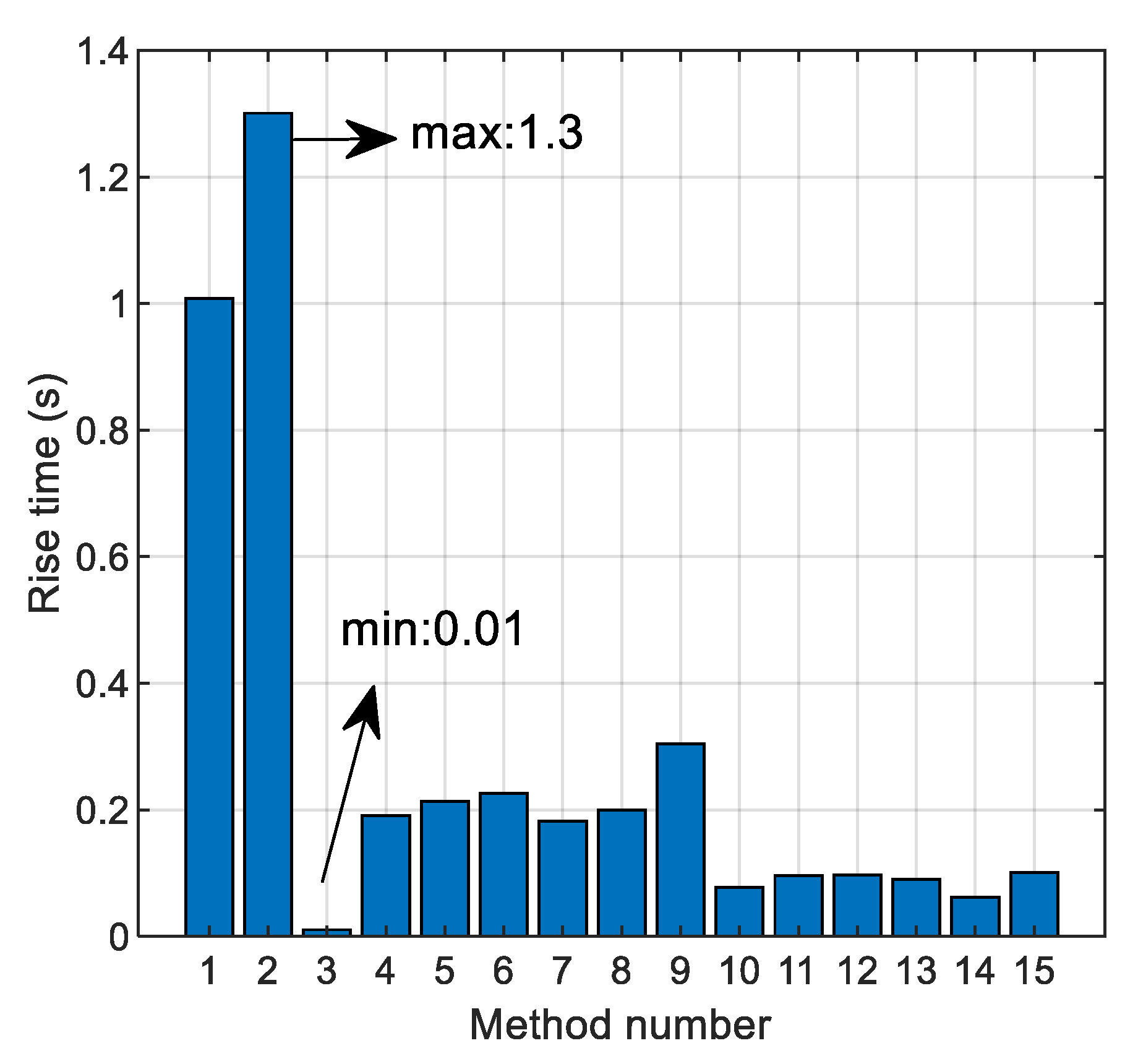
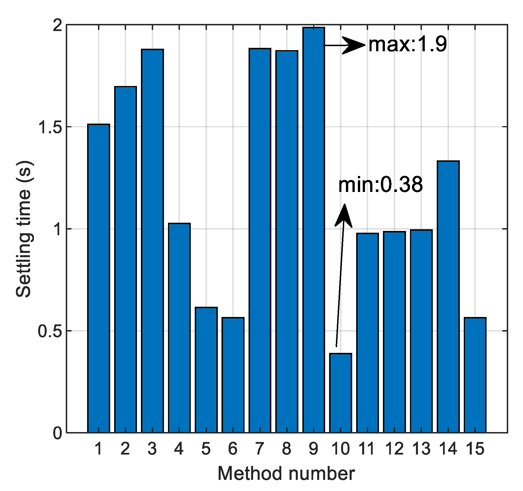
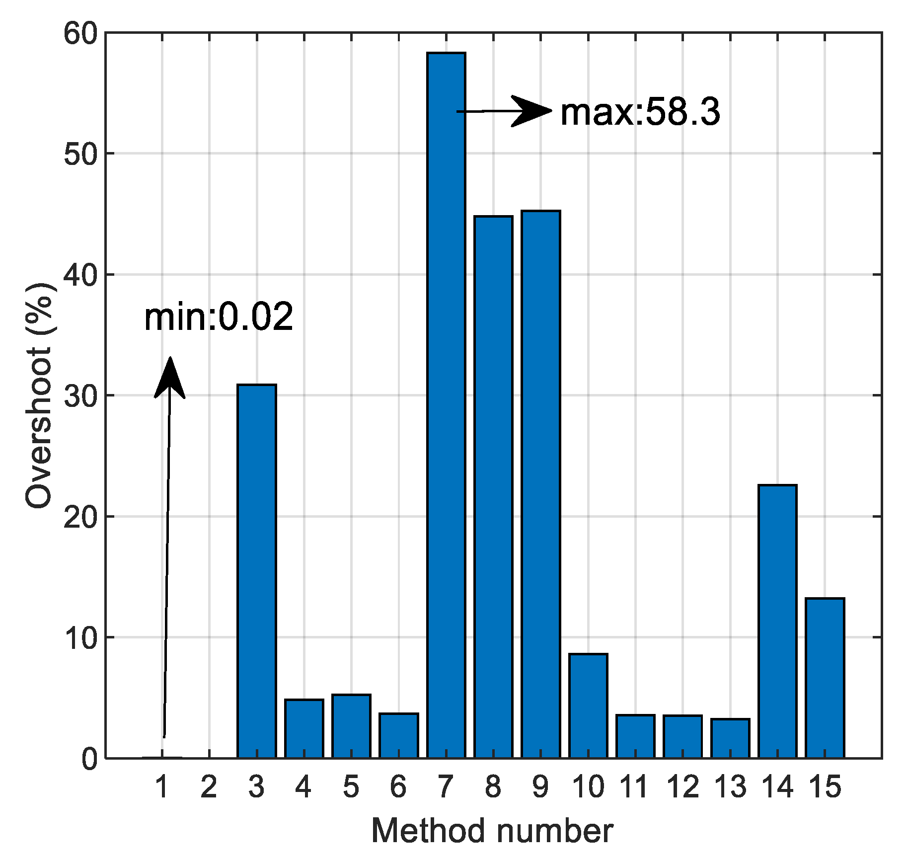
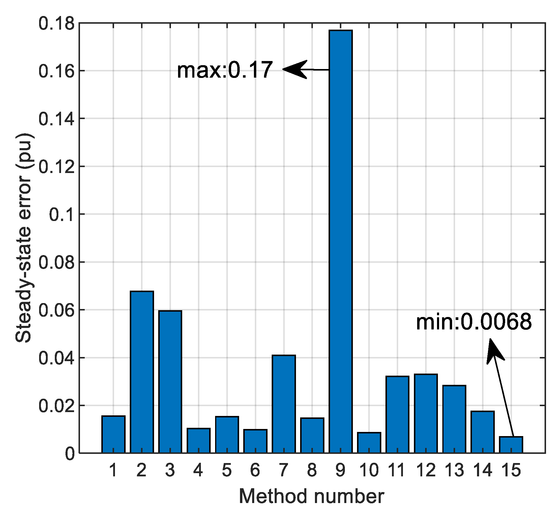
It is important to mention that the transient response parameters presented in the table are the calculated values obtained by carrying out the simulations with the given FOPID parameters. In order to conduct the graphical comparison between given references in terms of the transient response parameters, Figure 6, Figure 7, Figure 8 and Figure 9 present rise time, settling time, overshoot, and steady-state error, respectively, for each method from Table 3.

The process of the optimization of the FOPID parameters highly depends on the chosen objective function that has to be minimized (or maximized). Considering the importance of the objective function, the list of different used functions is given in

Table 4. The list of the used objective functions.

Objective Function	Reference
$OF=w_1\cdot OS+w_2\cdot t_r+w_3\cdot t_s+w_4\cdot E_{ss}+{\displaystyle \int \left(w_5\cdot |e(t)|+w_6\cdot V_f{(t)}^2\right)}dt+\frac{w_7}{P_m}+\frac{w_8}{G_m}$	[4]
$J_1={\omega }_{gc},J_2=P_m$	[5]
$IAE={\displaystyle \int |e(t)|dt}$	[6]
$ZLG=(1-e^{-\beta })\cdot (OS+E_{ss})+e^{-\beta }\cdot \left(t_s-t_r\right)$	[7,10]
$J_1={\displaystyle \int t{e}^2(t)dt},J_2={\displaystyle \int \mathsf{\Delta }{u}^2(t)dt},J_3={\displaystyle \int t{e_{load}}^2(t)dt}$	[8]
$J_1=IAE,J_2=1000|E_{ss}|,J_3=t_s$	[9]
$OF=w_1\cdot OS+w_2\cdot t_s+w_3\cdot E_{ss}+w_4{\displaystyle \int |e(t)|}dt+w_5{\displaystyle \int u^2(t)dt}$	[11]
$OF={(w_1\cdot OS)}^2+w_2{t_s}^2+\frac{w_3}{{\left(\max \_dv\right)}^2}$	[11]
$ITAE={\displaystyle \int t|e(t)|dt}$	[12]

. It can be observed that certain authors use a single objective function [4,6,7,10,11,12], while others perform multi-objective optimization [5,8,9].

In the previous table, e is the error signal (the difference between the reference voltage and the terminal voltage), V_f is the voltage of the generator field winding, ω_gc is the gain crossover frequency, u is the control signal (the output of the controller), e_load is the error signal when load disturbances are present, and max_dv is the maximum point of the voltage signal derivative. The weighting coefficients are marked as w₁, w₂, w₃, ..., w₈.

5. Proposed Chaotic-Yellow Saddle Goatfish Algorithm

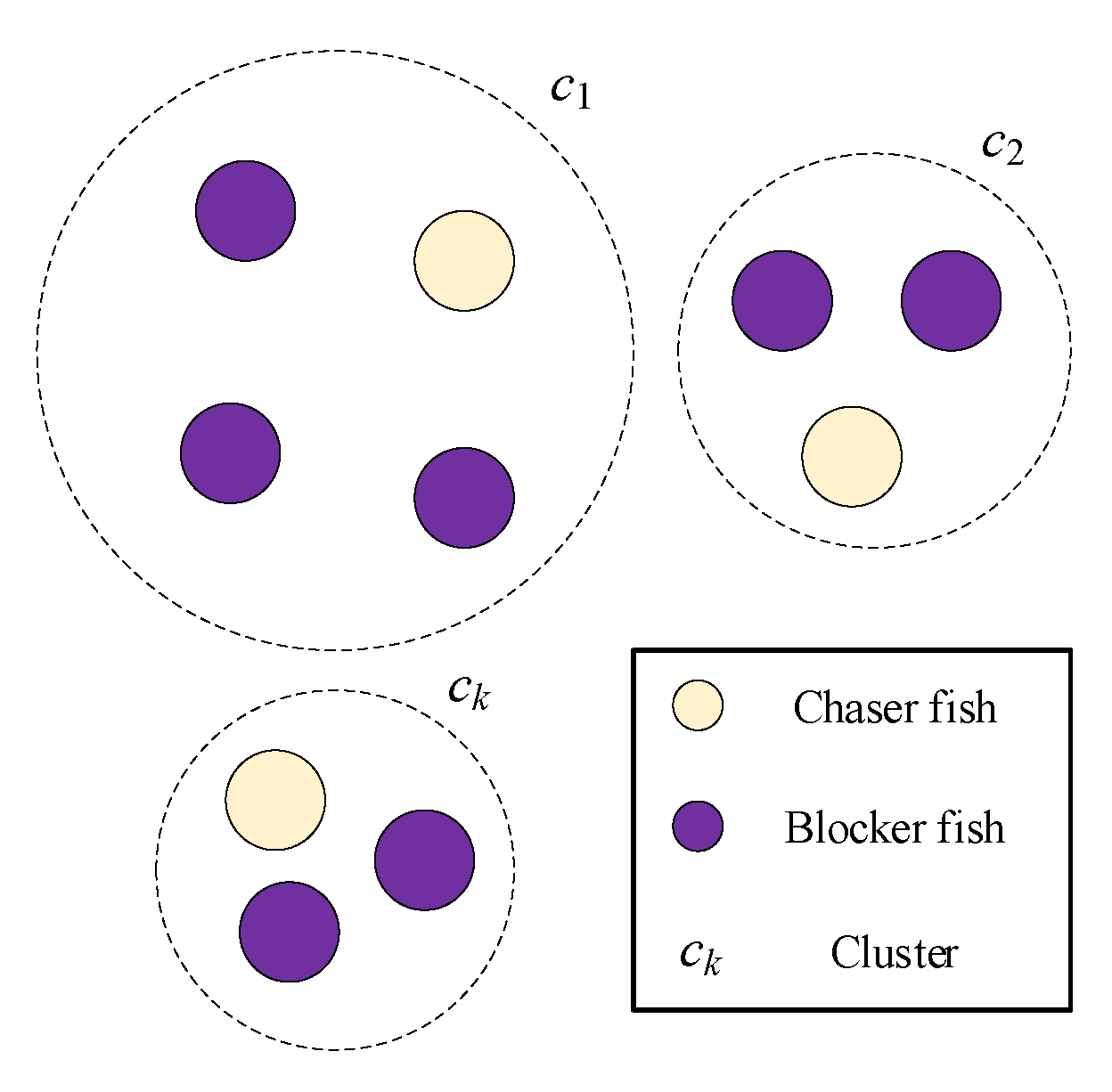
The development of the Yellow Saddle Goatfish Algorithm (YSGA) is based on the model of the hunting process by a group of yellow saddle goatfishes, as proposed in [23]. According to this approach, the whole population of the fishes is split into sub-populations. Each sub-population has one fish that is called a chaser, while the others are called blockers. Also, the search space of the possible solutions for the optimization problem is represented by the hunting area of the goatfishes.

The first step of the YSGA is the initialization of the population. Assuming that a population P consists of m goatfishes (P = {p₁, p₂, ..., p_m}), each goatfish is initialized randomly between the low boundary (b^L) and the high boundary (b^H) of the search space [23]:

$$p_i=rand\cdot \left(b^H-b^L\right)+b^L,i=1,2,\dots ,m,$$

(11)

where rand is a vector of random numbers between 0 and 1. It is very important to mention that p_i is a vector that consists of n decision variables (variables that are being optimized). Furthermore, b^L and b^H are also vectors that represent lower and upper boundaries for each decision variable.

According to (11), the initialization process of the original YSGA proposed in [23] is random, which does not ensure a good starting point in the optimization process. Namely, metaheuristic algorithms have extremely sensitive dependence on the initial conditions, so the improvements in this part may have a great effect on the overall performance of an algorithm. The idea of introducing Chaotic maps into the metaheuristic algorithms in order to replace the random parameters that appear in the algorithm is shown in [26,27,28]. Among the most interesting approaches are the ones presented in [29,30,31], where the random population is replaced with the population generated by Chaotic algorithm with different maps. There are many existing Chaotic maps, such as circle map, cubic map, Gauss map, ICMIC map, logistic map, sinusoidal map, and so on. In order to examine the performances of the mentioned maps, many authors provide a mutual comparison of the different maps [29,30,31,32,33]. Concretely, the comparison is carried out by solving concrete optimization problems employing the different Chaotic maps. The existing studies demonstrate that the logistic mapping is the most convenient to use, due to the better computational efficiency than other mentioned Chaotic maps [29,30,31,32,33].

Based on the previous analysis, this paper introduces the initialization of the population using Chaotic Logistic Mapping [24]. Thus, the random initialization is given by (11), which is proposed by the original YSGA algorithm, is replaced by the initialization provided as a result of Chaotic Logistic Mapping. The proposed model of the initialization of the population is described by (12) and (13). Firstly, vectors y_i that are the products of Logistic Mapping are introduced as follows:

$$\begin{array}{l}{y}_1=rand,\\ y_{i+1}=\mu \cdot y_i\cdot (1-y_i),i=1,2,\dots m,\end{array}$$

(12)

where rand stands for a vector of random numbers in the interval [0,1], and μ is the coefficient that is chosen to be 4 in this study. In this manner, we gave the chaotic character of the basic Yellow Saddle Goatfish Algorithm.

Afterward, initialization in C-YSGA is realized according to the following Equation:

$$p_i=y_i\cdot \left(b^H-b^L\right)+b^L,i=1,2,\dots ,m.$$

(13)

Before starting the process of the hunt, the whole population must be divided into sub-populations or clusters. Each of the k clusters c_k has a chaser fish Φ_l and the blocker fish φ_g. Clustering can be made using any of the clustering algorithms. However, the YSGA algorithm uses the K-means clustering algorithm in order to divide the population, as it is described in [23] in detail. The cluster organization of the population is depicted in Figure 10.

The chaser fish of each cluster is the one with the best fitness value. The first step of the hunting process is to update the position of the chaser fish. If the current position is denoted as Φ_l^t, the updated position is Φ_l^t+1, and the best chaser fish from all clusters is Φ_best^t, where t represents the number of the iteration; the updated law is given by the following Equation:

$${{\mathsf{\Phi }}_l}^{t+1}={{\mathsf{\Phi }}_l}^t+\alpha \left(\frac{u}{{|v|}^{1/\beta }}\right)\left({{\mathsf{\Phi }}_l}^t-{{\mathsf{\Phi }}_{best}}^t\right),$$

(14)

where α defines the step size (it is set to 1 in this study), and β is Levy index that is calculated as follows (t_max stands for the maximum number of iterations):

$$\beta =1.99+\raisebox{1ex}{$0.01t$}\!\left/ \!\raisebox{-1ex}{$t_{max}$}\right..$$

(15)

Parameters u and v from (14) are defined using the following equations:

$$u\sim N\left(0,{{\sigma }_u}^2\right),{\sigma }_u={\left(\frac{\mathsf{\Gamma }(1+\beta )\cdot \sin \frac{\beta \pi }{2}}{\mathsf{\Gamma }(1+\beta )\cdot \beta \cdot 2^{\left(\beta -1\right)/2}}\right)}^{1/\beta },$$

(16)

$$v\sim N\left(0,{{\sigma }_v}^2\right),{\sigma }_v=1,$$

(17)

where Γ stands for Gamma function and N for normal distribution. In order to update the position of the best chaser fish from all clusters, it is necessary to use (18) instead of (14):

$${{\mathsf{\Phi }}_{best}}^{t+1}={{\mathsf{\Phi }}_{best}}^t+\alpha \left(\frac{u}{{|v|}^{1/\beta }}\right),$$

(18)

The next step in the optimization process is the update of the positions of the blocker fishes. The new position of the blocker fish φ_g^t+1 can be determined based on the following Equation:

$${{\phi }_g}^{t+1}=|r\cdot {\mathsf{\Phi }}_l-{{\phi }_g}^t|\cdot e^{b\rho }\cdot \cos \left(2\pi p\right)+{\mathsf{\Phi }}_l,$$

(19)

where ρ is a random number between a and 1, r is a random number between 0 and 1, and b is the constant that is set to be 1. The parameter a is called the exploitation factor and is linearly decreased from −1 to −2 during the iterations.

It is vital to keep in mind that during the optimization process, the exchange of roles may occur. Namely, if the blocker fish has a better fitness value than the chaser fish, they exchange the roles, and the blocker fish becomes a new chaser fish in the next iteration.

The YSGA model has the predefined parameter λ, which is called an overexploitation parameter. Precisely, if a solution is not improved in λ iterations, it is necessary to change an area of the hunt. Each goatfish, no matter if it is chaser or blocker, must change the hunting area according to the following Equation:

$${p_g}^{t+1}=\frac{{\mathsf{\Phi }}_{best}+{p_g}^t}{2},$$

(20)

where p_g^t and p_g^t+1 represent old and new positions of the goatfish, respectively. The whole described process is iteratively repeated until the maximum number of iterations is reached. The detailed description is provided with the pseudo-code presented in

Table 5. Pseudo-code of the proposed C-YSGA.

Pseudo-Code of the C-YSGA

Enter the input data: m, k, tmax, λ Initialize the population P using chaotic logistic mapping According to the fitness values determine Φbest Split the population into k clusters and determine the chaser fish Φl for each cluster while (t < tmax) for each cluster Update the position of the chaser fish and blocker fish Calculate the fitness value of every fish Exchange the roles if any blocker fish has better fitness value than the chaser fish Update the Φbest if the chaser fish has better fitness value If the fitness value of the chaser fish has not improved, increase the counter q by 1 If the counter q is higher than λ then apply the formula for the change of the zone end for t = t + 1 endwhile Φbest is the output result of the algorithm

.

This section is not mandatory but can be added to the manuscript if the discussion is unusually long or complicated.

6. Simulation Results

This section presents the results that are obtained by applying the proposed C-YSGA method to optimize the FOPID parameters of the AVR system.

Firstly, the formulation of the optimization problem is provided, including the novel objective function presented in this paper. Afterward, the convergence characteristics of the different optimization algorithms used in the literature are compared to the one obtained by C-YSGA in order to demonstrate the convergence superiority of the proposed algorithm. Furthermore, the comparison is conducted in terms of the step response of the AVR system, as well as in the cases of different kinds of uncertainties and disturbances in the system.

6.1. Formulation of the Optimization Problem

From (2), it can be seen that the FOPID is defined with 5 parameters, K_p, K_i, K_d, λ, and μ, which need to be optimized so that the controller satisfies the desired performances. The optimization process is guided by the objective function that defines the performances of the AVR system.

In order to provide a good quality transient response (for the reference step signal), we tested all of the previously used objective functions. However, none of the mentioned functions provide the appropriate system responses as they do not take into account all of the essential characteristics (time-domain parameters or frequency parameters). Furthermore, they do not give an appropriate compromise between all the critical time-domain parameters. On the other side, the objective functions that are based on frequency parameters have higher execution time, which makes the optimization process slower. Observing the different mathematical formulations of the objective functions presented in [4,7,10,11], the authors in this paper propose a novel objective function (21) that contains a smaller number of weighting coefficients, but also outperforms other objective functions in the literature:

$$OF=w_1\cdot {\displaystyle \int t|e(t)|}dt+w_{2}OS+w_3|E_{ss}|+w_4{t}_s.$$

(21)

Weighting coefficients are chosen carefully after many experiments, and the following values are considered in this paper: w₁ = 1, w₂ = 0.02, w₃ = 1, and w₄ = 5. The values of the coefficients are chosen after many experiments with different combinations. It can be seen that w₂ has a significantly lower value than the other three weighting coefficients. The reason for this is that the overshoot in (21) is given in percentage, and its value is always larger than the values of ITAE, settling time, and steady-state error. Concretely, from Table 3, it can be observed that the highest value of overshoot can go to 45%, while the settling time and the steady-state error reach maximum values of 1.9 s and 0.17 pu, respectively. However, it is very important to highlight that the presence of the FOPID controller can make the closed-loop system unstable. In order to surpass that, this paper uses optimization with constraints. In other words, each solution (each set of FOPID parameters) is first tested to examine if the obtained closed-loop system remains stable. If a certain solution makes the system unstable, it is automatically removed, ignoring its fitness value. The size of the population in the C-YSGA algorithm is selected to be 40, and the maximum number of iterations is 50. Also, the lower and upper boundary must be defined for each of the optimization variables. Taking into account previous studies related to this topic, the chosen boundaries that are used in this paper are presented in

Table 6. Boundaries of the optimization variables.

Parameter	Lower Bound	Upper Bound
Kp	1	2
Ki	0.1	1
Kd	0.1	0.4
λ	1	2
μ	1	2

.

By using the proposed C-YSGA method and the novel objective function depicted above, the optimal FOPID parameters are: K_p = 1.762, K_i = 0.897, K_d = 0.355, μ = 1.26, and λ = 1.032. The proposed method is compared with all methods presented in Table 3, and the results are provided in

Table 7. Comparison of the proposed method with other techniques from literature in terms of OF.

Method Number	Proposed	1	2	3	4	5	6	7
OF value	1.08	24.6	47.3	50	10.1	8.4	4.5	12.3
Method number	8	9	10	11	12	13	14	15
OF value	10.1	53.6	2.3	4.8	4.8	3	9.8	3.1

where the best value is in bold. Note, the best solutions of each method, as it is shown in Table 3, are applied with the proposed fitness function given by (21). It is clear that the new fitness function proposed in this paper has the lowest value when the FOPID parameters obtained by C-YSGA algorithm are used.

6.2. Convergence Characteristics

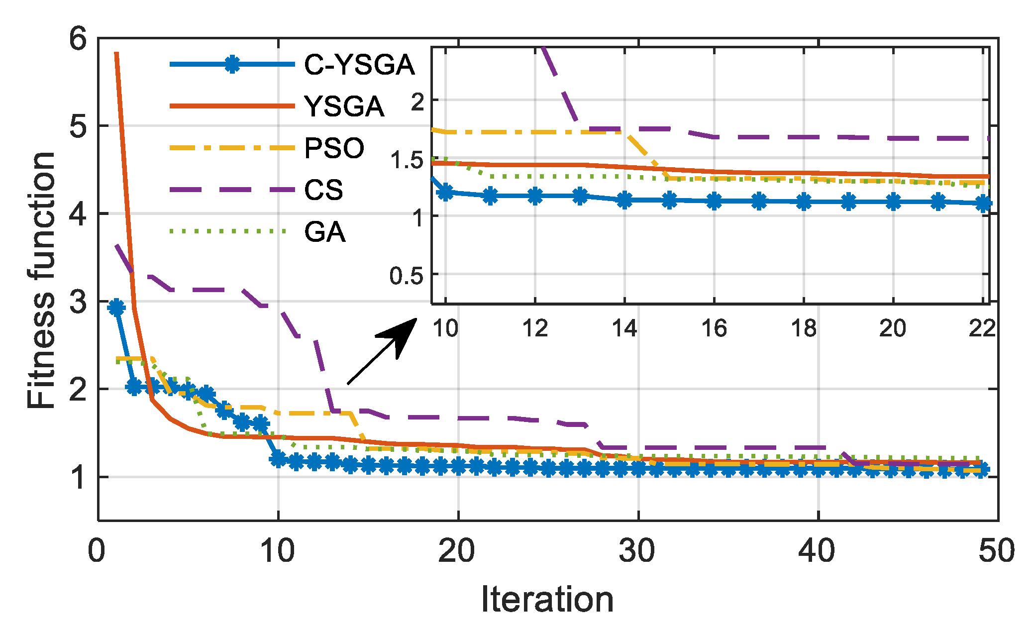
The main goal of hybridizing the concepts of two algorithms (classical YSGA and chaotic logistic mapping) is to accelerate the convergence speed of the original algorithm. Due to the fact that the initial population of the C-YSGA is not selected randomly, but it is the product of the chaotic logistic mapping, it is expected that the proposed algorithm will reach the optimal solution for the least number of iterations. In order to demonstrate that, the original YSGA algorithm, as well as PSO [11], CS [10], and GA [5] algorithms have been implemented to determine the optimal FOPID parameters using the proposed objective function (21). The convergence curves of all mentioned algorithms demonstrate that the C-YSGA algorithm converges in a minimum number of iterations (approximately 10) compared to the other algorithms, as it is depicted in Figure 11. In this figure, the convergence characteristics represent the mean value of convergence characteristics when we started all the algorithms multiple times. Therefore, the chaotic improvement of the standard YSGA algorithm enables obtaining better convergence characteristics. In that manner, it is demonstrated that Chaotic maps, in combination with the metaheuristic algorithm, improves the initial position, which is very important for the convergence speed of the algorithm.

6.3. Step Response

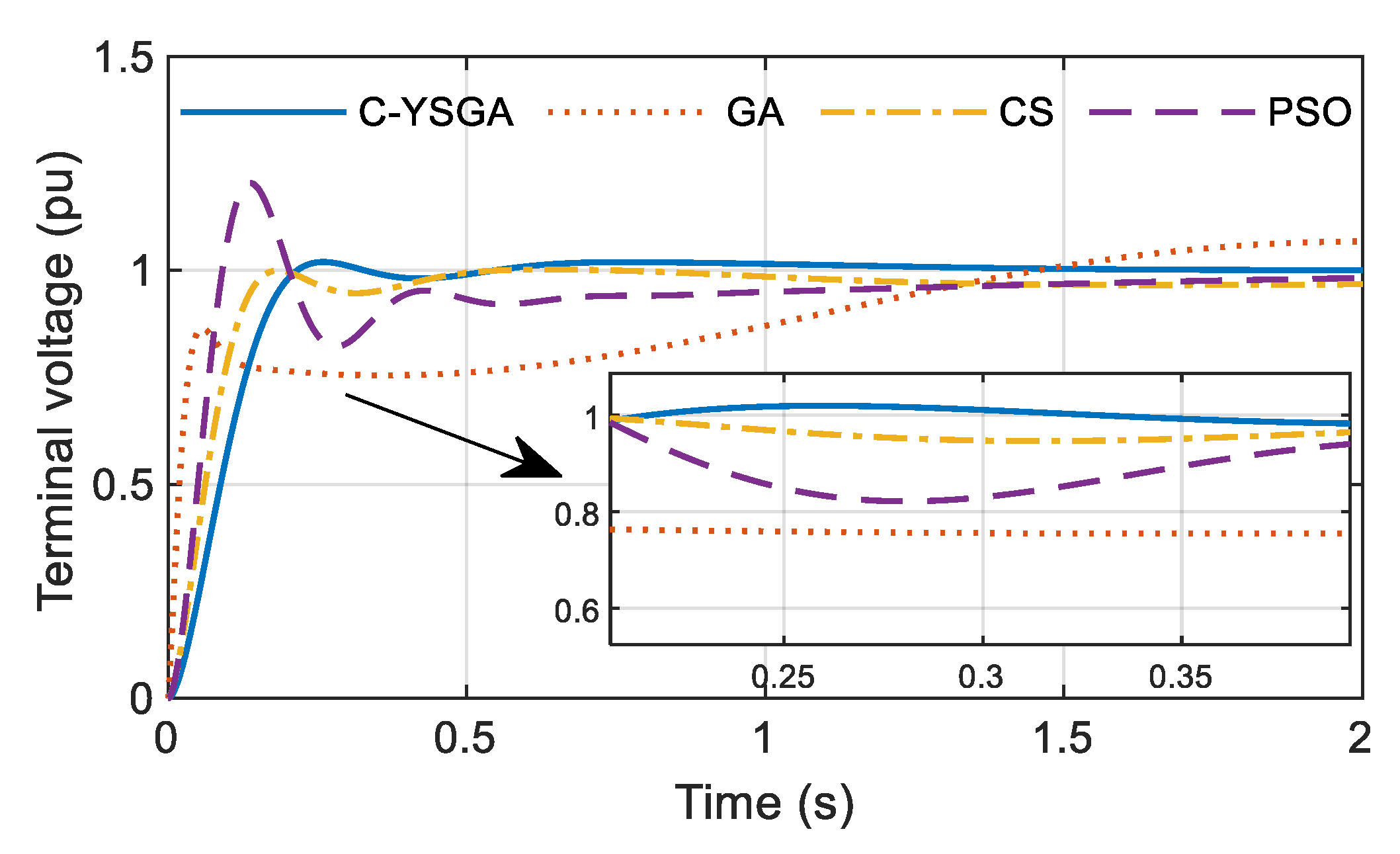
Among all the presented results in Table 3, for the comparison with the proposed C-YSGA, the papers [5,10,11] are chosen. The main indicators of the step response quality-rise time, settling time, overshoot, and steady state-error, as well as the obtained FOPID parameters, are presented in

Table 8. Comparison of the transient response parameters.

Algorithm	Kp	Ki	Kd	μ	λ	tr (s)	ts (s)	OS (%)	|Ess| (pu)
C-YSGA	1.7775	0.9463	0.3525	1.2606	1.1273	0.1347	0.2	1.89	0.0009
PSO [11]	1.5338	0.6523	0.9722	1.209	0.9702	0.0614	1.3313	22.58	0.0175
CS [10]	2.549	0.1759	0.3904	1.38	0.97	0.0963	0.9774	3.56	0.0321
GA [5]	0.9632	0.3599	0.2816	1.8307	0.5491	1.3008	1.6967	6.99	0.0677

, the best values are marked in bold.

Additionally, the step response of the AVR system with FOPID parameters from Table 4 is shown in Figure 12. Undoubtedly, it can be concluded that the FOPID controller tuned by the proposed C-YSGA method provides better transient response compared to the other considered algorithms. Precisely, the settling time, the overshoot, and the absolute value of the steady-state error have the least values when the C-YSGA is used, while the rise time has a very low value. Taking a look into the previous table, it can be seen that the overshoot with the PSO algorithm [11] is 22%, which is an unacceptably big value. Similarly, the rise time and the settling time with the GA algorithm are larger than 1 s, which makes the voltage response extremely slow.

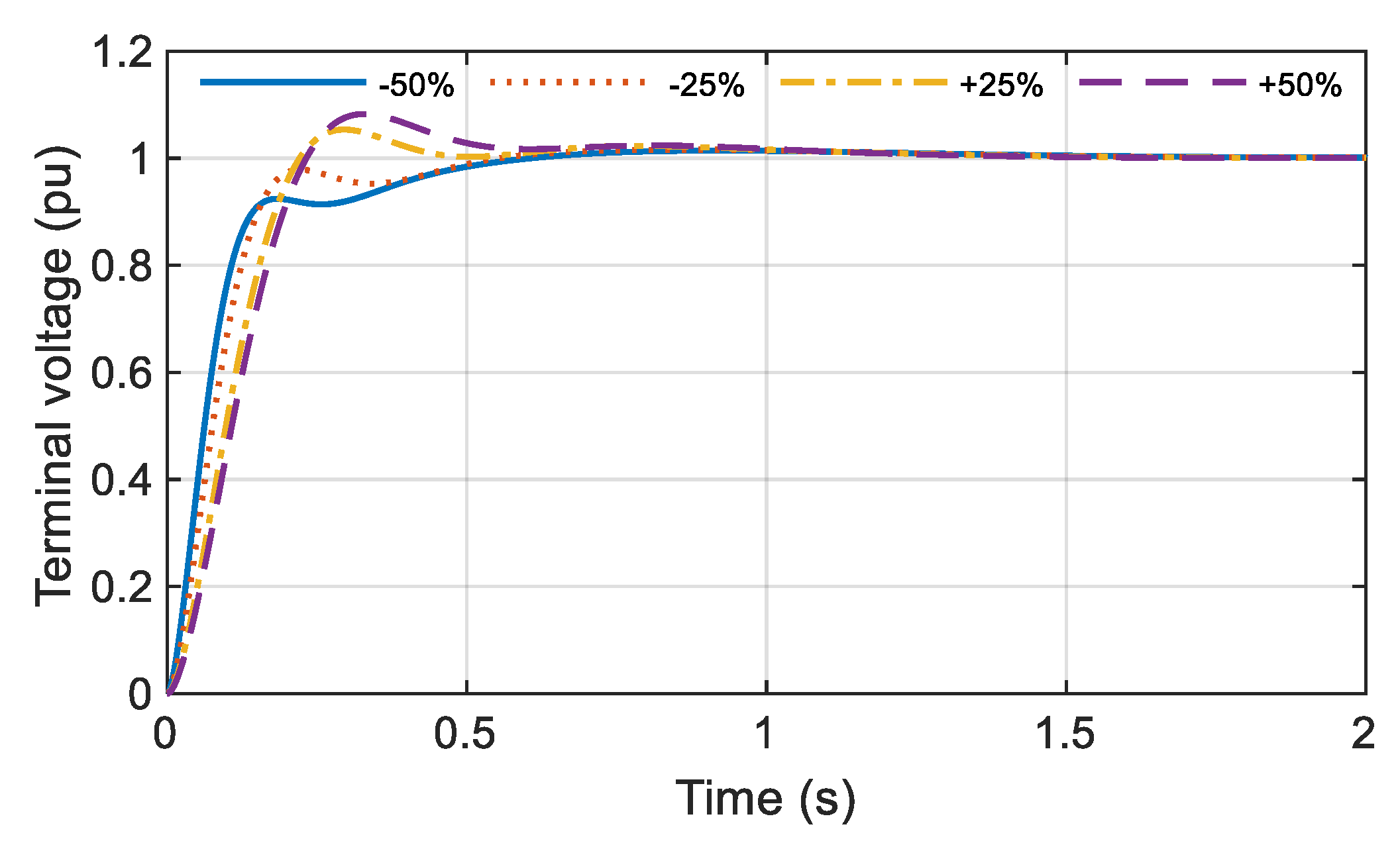
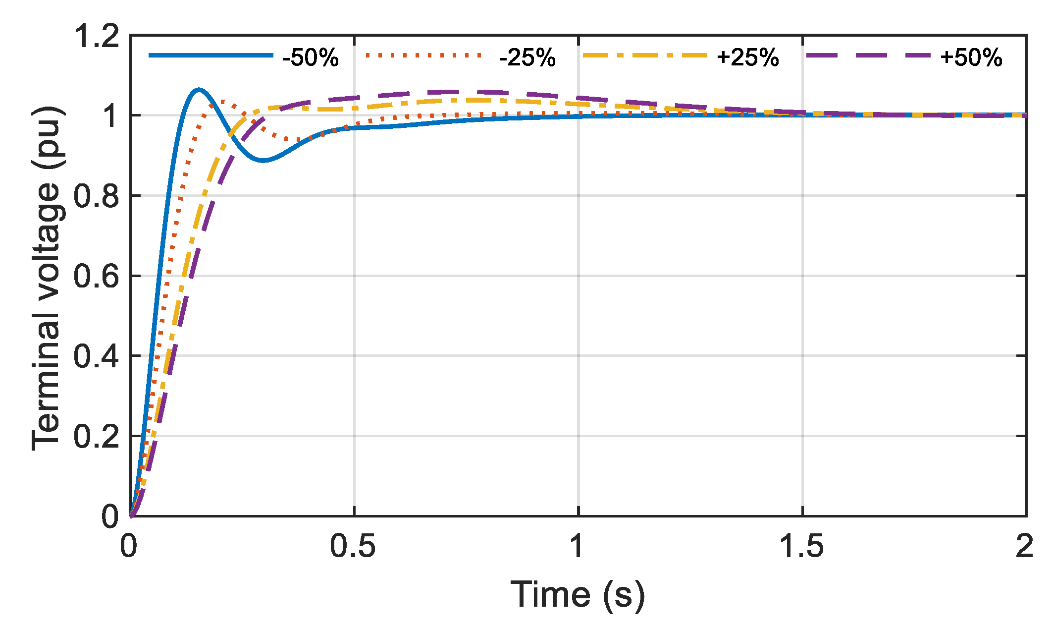
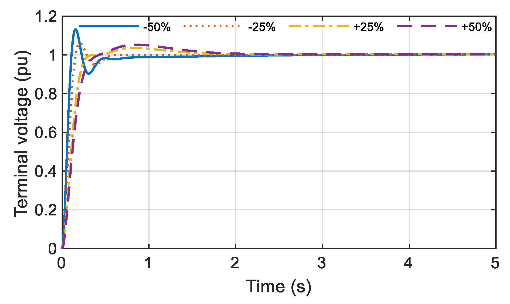
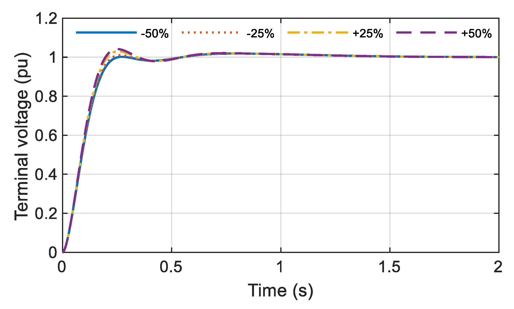
6.4. Robustness Analysis

The analysis in the previous section is conducted under the nominal conditions. However, it may occur that the components of the AVR system change their parameters. One of the tasks of the FOPID controller is to ensure the stability of the system and the high quality of the step response in the case of the sudden change in the parameters’ values. To that end, the robustness analysis of the AVR system with the C-YSGA FOPID controller is conducted, and the results are presented in Figure 13, Figure 14, Figure 15 and Figure 16. Precisely, the study is carried out for the change of time constants T_A, T_E, T_G, and T_S from −50% to +50% of the nominal value, in steps of 25%. The step response of the AVR system is shown in Figure 13, Figure 14, Figure 15 and Figure 16.

The results of the previous analysis prove that the C-YSGA FOPID controller makes the AVR system very robust to the changes of each parameter. It is observed that the step response does not deviate a lot compared to the nominal conditions.

6.5. Rejection of the Disturbances

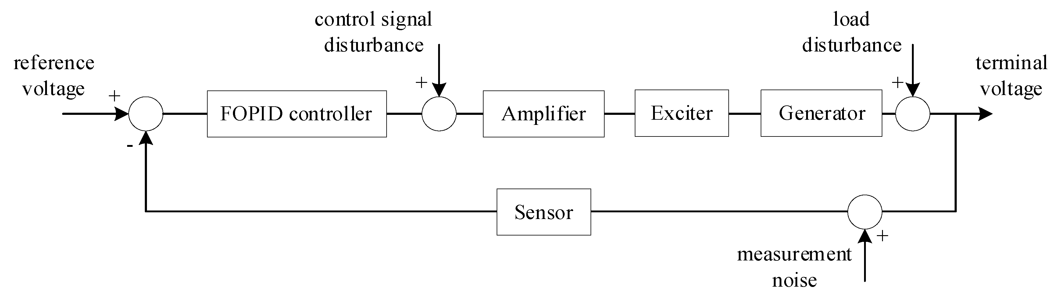
The ability of the FOPID controller to cope with the different disturbances is analyzed by introducing three kinds of disturbances into the AVR system: control signal disturbance, load disturbance, and measurement noise. The block diagram of the AVR with considered disturbances is depicted in Figure 17, while their detailed description is given as follows:

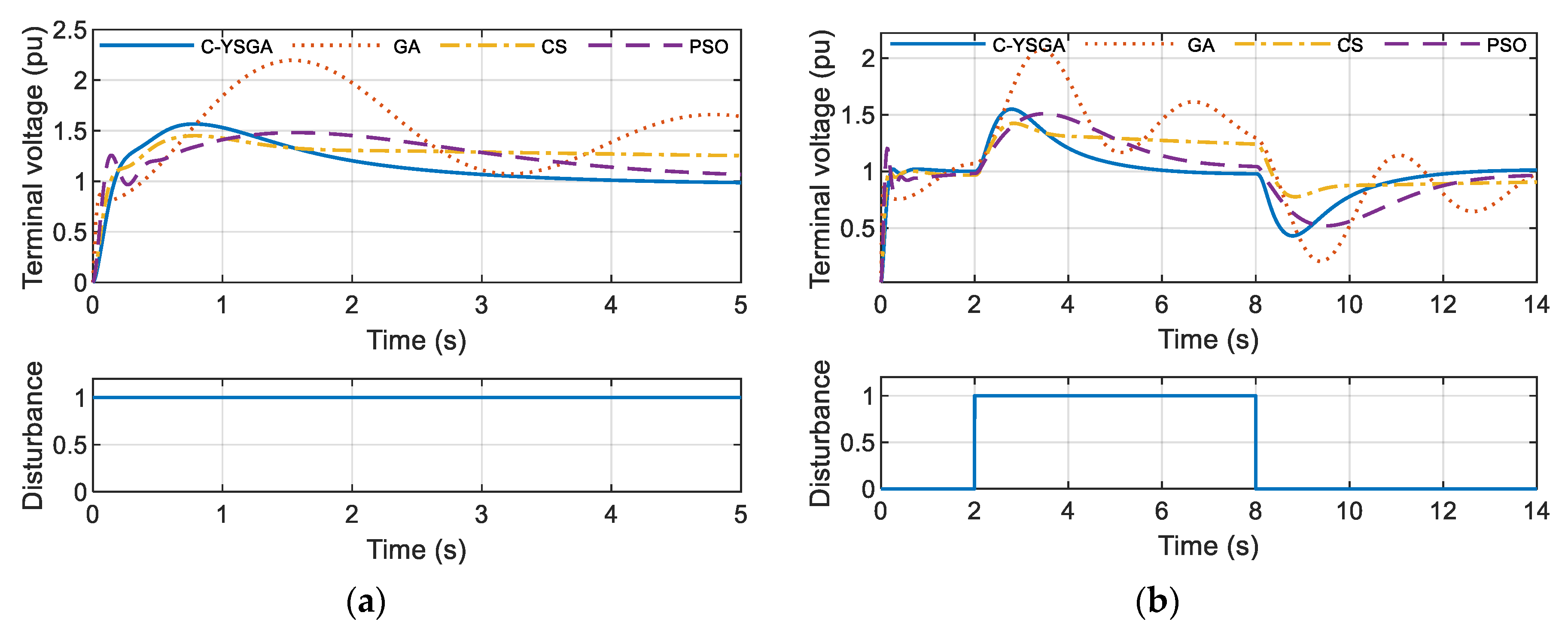
• One of the most common disturbances not only in the AVR system but generally in every control system is control signal disturbance. In this subsection, the obtained C-YSGA FOPID controller is compared with FOPID controllers tuned by PSO [11], CS [10], and GA [5] algorithms. Control signal disturbance is presented as a constant step signal in the first case, and in the second case as a step signal that lasts from t = 2 s to t = 8 s. Step responses of the AVR system are shown in Figure 18 for both cases.
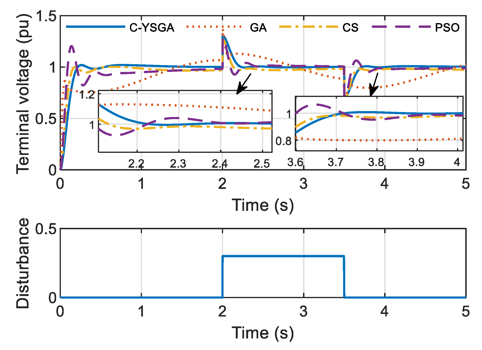
• Afterward, the load disturbance that is specific mainly for AVR systems is presented. Similarly to control signal disturbance, it is modeled as a step signal that lasts from t = 2 s to t = 3.5 s. The obtained step responses, in this case, are shown in Figure 19.
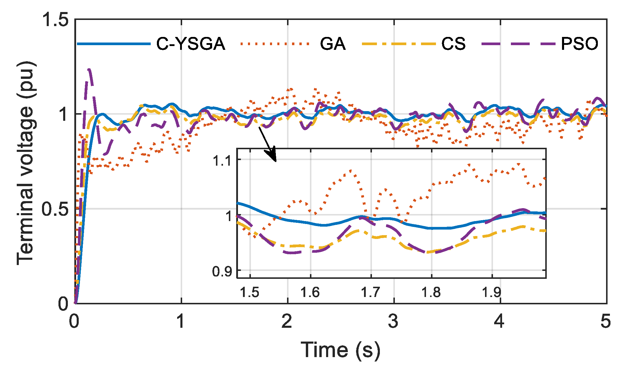
• The last type of disturbance is measurement noise, which is modeled as white Gaussian noise with the power 0.0001 dBW. Figure 20 presents the step responses of the AVR system when the measurement noise is present.

Based on the previous figures, it is obvious that the FOPID controller whose parameters are optimized by using a novel C-YSGA algorithm provides a significantly better ability to reject different types of disturbances. Comparison is conducted with some of the most popular and most used algorithms, whose performances, in this case, are remarkably weaker than the proposed method. To be more precise, from Figure 18 and Figure 19, it can be noted that the voltage does not reach its nominal value after the disturbance is introduced, when the controllers presented in [5,10,11] are used. Such fluctuations in the terminal voltage, caused by the inability of the controller to reject the disturbance, can present a major problem for the consumers of the electrical energy. Unlike them, the FOPID controller tuned by using C-YSGA provides a very stable level of the terminal voltage, whose value reaches the nominal value in a very short period after the disturbance in the system occurs.

7. Conclusions

This paper proposes the novel optimization algorithm in order to optimize the FOPID controller parameters in the AVR system. The proposed algorithm presents the compound of the Yellow Saddle Goatfish Algorithm (YSGA) and Chaotic Logistic mapping to obtain the innovative Chaotic-Yellow Saddle Goatfish Algorithm (C-YSGA). Instead of random initialization of the population, as in many existing metaheuristic algorithms, Chaotic Logistic mapping is used to determine the initial point in the optimization process. It is proved in the paper that such an approach significantly accelerates the convergence of the algorithm. Furthermore, to determine optimal FOPID controller parameters, a new objective function is presented. The results obtained by applying the proposed algorithm with the new objective function introduced in this paper provide significantly better voltage response of the AVR system compared to other considered algorithms. The robustness of the AVR system with such an obtained FOPID controller is tested by changing the AVR system’s parameters. It is shown that in all examined cases, the step response of the AVR system has extremely small deviations compared to the nominal case, which means the system is robust to the uncertainties in the system. Moreover, three very often disturbances are introduced into the system, and the system’s behavior with different FOPID controllers is analyzed. The mutual comparison shows that the C-YSGA FOPID controller is by far the best in rejecting all considered types of disturbances.

We think that in this way, the algorithm is improved, no matter what optimization problem is considered. In this paper, we tested its applicability and efficiency on the problem of optimal FOPID design. However, at the moment, we are working on proving its superiority over other literature known methods for solving the synchronous machine parameters estimation problem. To that goal, we consider field and armature current waveforms during the short circuit test.