Article

dCATCH—A Numerical Package for d-Variate near G-Optimal Tchakaloff Regression via Fast NNLS

Department of Mathematics “Tullio Levi Civita”, University of Padova, Via Trieste 63, 35131 Padova, Italy
*
Author to whom correspondence should be addressed.
Mathematics 2020, 8(7), 1122; https://doi.org/10.3390/math8071122
Submission received: 11 June 2020 / Revised: 5 July 2020 / Accepted: 7 July 2020 / Published: 9 July 2020
(This article belongs to the Special Issue Numerical Methods)

Abstract

:
We provide a numerical package for the computation of a d-variate near G-optimal polynomial regression design of degree m on a finite design space X R d , by few iterations of a basic multiplicative algorithm followed by Tchakaloff-like compression of the discrete measure keeping the reached G-efficiency, via an accelerated version of the Lawson-Hanson algorithm for Non-Negative Least Squares (NNLS) problems. This package can solve on a personal computer large-scale problems where c a r d ( X ) × dim ( P 2 m d ) is up to 10 8 10 9 , being dim ( P 2 m d ) = 2 m + d d = 2 m + d 2 m . Several numerical tests are presented on complex shapes in d = 3 and on hypercubes in d > 3 .

1. Introduction

In this paper we present the numerical software package dCATCH [1] for the computation of a d-variate near G-optimal polynomial regression design of degree m on a finite design space X R d . In particular, it is the first software package for general-purpose Tchakaloff-like compression of d-variate designs via Non-Negative Least Squares (NNLS), freely available on the Internet. The code is an evolution of the codes in Reference [2] (limited to d = 2 , 3 ), with a number of features tailored to higher dimension and large-scale computations. The key ingredients are:
  • use of d-variate Vandermonde-like matrices at X in a discrete orthogonal polynomial basis (obtained by discrete orthonormalization of the total-degree product Chebyshev basis of the minimal box containing X), with automatic adaptation to the actual dimension of P m d ( X ) ;
  • few tens of iterations of the basic Titterington multiplicative algorithm until near G-optimality of the design is reached, with a checked G-efficiency of say 95 % (but with a design support still far from sparsity);
  • Tchakaloff-like compression of the resulting near G-optimal design via NNLS solution of the underdetermined moment system, with concentration of the discrete probability measure by sparse re-weighting to a support X , of cardinality at most P 2 m d ( X ) , keeping the same G-efficiency;
  • iterative solution of the large-scale NNLS problem by a new accelerated version of the classical Lawson-Hanson active set algorithm, that we recently introduced in Reference [3] for 2 d and 3 d instances and here we validate on higher dimensions.
Before giving a more detailed description of the algorithm, it is worth recalling in brief some basic notions of optimal design theory. Such a theory has its roots and main applications within statistics, but also strong connections with approximation theory. In statistics, a design is a probability measure μ supported on a (discrete or continuous) compact set Ω R d . The search for designs that optimize some properties of statistical estimators (optimal designs) dates back to at least one century ago, and the relevant literature is so wide and still actively growing and monographs and survey papers are abundant in the literature. For readers interested in the evolution and state of the art of this research field, we may quote, for example, two classical treatises such as in References [4,5], the recent monograph [6] and the algorithmic survey [7], as well as References [8,9,10] and references therein. On the approximation theory side we may quote, for example, References [11,12].
The present paper is organized as follows—in Section 2 we briefly recall some basic concepts from the theory of Optimal Designs, for the reader’s convenience, with special attention to the deterministic and approximation theoretic aspects. In Section 3 we present in detail our computational approach to near G-optimal d-variate designs via Caratheodory-Tchakaloff compression. All the routines of the dCATCH software package here presented, are described. In Section 4 we show several numerical results with dimensions in the range 3–10 and a Conclusions section follows.
For the reader’s convenience we also display Table 1 and Table 2, describing the acronyms used in this paper and the content (subroutine names) of the dCATCH software package.

2. G-Optimal Designs

Let P m d ( Ω ) denote the space of d-variate real polynomials of total degree not greater than n, restricted to a (discrete or continuous) compact set Ω R d , and let μ be a design, that is, a probability measure, with s u p p ( μ ) Ω . In what follows we assume that s u p p ( μ ) is determining for P m d ( Ω ) [13], that is, polynomials in P m d vanishing on s u p p ( μ ) vanish everywhere on Ω .
In the theory of optimal designs, a key role is played by the diagonal of the reproducing kernel for μ in P m d ( Ω ) (also called the Christoffel polynomial of degree m for μ )
K m μ ( x , x ) = j = 1 N m p j 2 ( x ) , N m = dim ( P m d ( Ω ) ) ,
where { p j } is any μ -orthonormal basis of P m d ( Ω ) . Recall that K m μ ( x , x ) can be proved to be independent of the choice of the orthonormal basis. Indeed, a relevant property is the following estimate of the L -norm in terms of the L μ 2 -norm of polynomials
p L ( Ω ) max x Ω K m μ ( x , x ) p L μ 2 ( Ω ) , p P m d ( Ω ) .
Now, by (1) and μ -orthonormality of the basis we get
Ω K m μ ( x , x ) d μ = j = 1 N m Ω p j 2 ( x ) d μ = N m ,
which entails that max x Ω K m μ ( x , x ) N m .
Then, a probability measure μ * = μ * ( Ω ) is then called a G-optimal design for polynomial regression of degree m on Ω if
min μ max x Ω K m μ ( x , x ) = max x Ω K m μ * ( x , x ) = N m .
Observe that, since Ω K m μ ( x , x ) d μ = N m for every μ , an optimal design has also the following property K m μ * ( x , x ) = N m , μ * -a.e. in Ω .
Now, the well-known Kiefer-Wolfowitz General Equivalence Theorem [14] (a cornerstone of optimal design theory), asserts that the difficult min-max problem (4) is equivalent to the much simpler maximization problem
max μ d e t ( G m μ ) , G m μ = Ω ϕ i ( x ) ϕ j ( x ) d μ 1 i , j N m ,
where G m μ is the Gram matrix (or information matrix in statistics) of μ in a fixed polynomial basis { ϕ i } of P m d ( Ω ) . Such an optimality is called D-optimality, and ensures that an optimal measure always exists, since the set of Gram matrices of probability measures is compact and convex; see for example, References [5,12] for a general proof of these results, valid for continuous as well as for discrete compact sets.
Notice that an optimal measure is neither unique nor necessarily discrete (unless Ω is discrete itself). Nevertheless, the celebrated Tchakaloff Theorem ensures the existence of a positive quadrature formula for integration in d μ * on Ω , with cardinality not exceeding N 2 m = dim ( P 2 m d ( Ω ) ) and which is exact for all polynomials in P 2 m d ( Ω ) . Such a formula is then a design itself, and it generates the same orthogonal polynomials and hence the same Christoffel polynomial of μ * , preserving G-optimality (see Reference [15] for a proof of Tchakaloff Theorem with general measures).
We recall that G-optimality has two important interpretations in terms of statistical and deterministic polynomial regression.
From a statistical viewpoint, it is the probability measure on Ω that minimizes the maximum prediction variance by polynomial regression of degree m, cf. for example, Reference [5].
On the other hand, from an approximation theory viewpoint, if we call L m μ * the corresponding weighted least squares projection operator L ( Ω ) P m d ( Ω ) , namely
f L m μ * f L μ * 2 ( Ω ) = min p P m d ( Ω ) f p L μ * 2 ( Ω ) ,
by (2) we can write for every f L ( Ω )
L m μ * f L ( Ω ) max x Ω K m μ * ( x , x ) L m μ * f L μ * 2 ( Ω ) = N m L m μ * f L μ * 2 ( Ω ) N m f L μ * 2 ( Ω ) N m f L ( Ω ) ,
(where the second inequality comes from μ * -orthogonality of the projection), which gives
L m μ * = sup f 0 L m μ * f L ( Ω ) f L ( Ω ) N m ,
that is a G-optimal measure minimizes (the estimate of) the weighted least squares uniform operator norm.
We stress that in this paper we are interested in the fully discrete case of a finite design space Ω = X , so that any design μ is identified by a set of positive weights (masses) summing up to 1 and integrals are weighted sums.

3. Computing near G-Optimal Compressed Designs

Since in the present context we have a finite design space Ω = X = { x 1 , , x M } R d , we may think a design μ as a vector of non-negative weights u = ( u 1 , , u M ) attached to the points, such that u 1 = 1 (the support of μ being identified by the positive weights). Then, a G-optimal (or D-optimal) design μ * is represented by the corresponding non-negative vector u * . We write K m u ( x , x ) = K m μ ( x , x ) for the Christoffel polynomial and similarly for other objects (spaces, operators, matrices) corresponding to a discrete design. At the same time, L ( Ω ) = ( X ) , and L μ 2 ( Ω ) = u 2 ( X ) (a weighted 2 functional space on X) with f u 2 ( X ) = i = 1 M u i f 2 ( x i ) 1 / 2 .
In order to compute an approximation of the desired u * , we resort to the basic multiplicative algorithm proposed by Titterington in the ’70s (cf. Reference [16]), namely
u i ( k + 1 ) = u i ( k ) K m u ( k ) ( x i , x i ) N m , 1 i M , k = 0 , 1 , 2 , ,
with initialization u ( 0 ) = ( 1 / M , , 1 / M ) T . Such an algorithm is known to be convergent sublinearly to a D-optimal (or G-optimal by the Kiefer-Wolfowitz Equivalence Theorem) design, with an increasing sequence of Gram determinants
d e t ( G m u ( k ) ) = d e t ( V T d i a g ( u ( k ) ) V ) ,
where V is a Vandermonde-like matrix in any fixed polynomial basis of P m d ( X ) ; cf., for example, References [7,10]. Observe that u ( k + 1 ) is indeed a vector of positive probability weights if such is u ( k ) . In fact, the Christoffel polynomial K m u ( k ) is positive on X, and calling μ k the probability measure on X associated with the weights u ( k ) we get immediately i u i ( k + 1 ) = 1 N m i u i ( k ) K m u ( k ) ( x i , x i ) = 1 N m X K m u ( k ) ( x , x ) d μ k = 1 by (3) in the discrete case Ω = X .
Our implementation of (7) is based on the functions
  • C = dCHEBVAND ( n , X )
  • [ U , j v e c ] = dORTHVAND ( n , X , u , j v e c )
  • [ p t s , w ] = dNORD ( m , X , g t o l )
The function dCHEBVAND computes the d-variate Chebyshev-Vandermonde matrix C = ( ϕ j ( x i ) ) R M × N n , where { ϕ j ( x ) } = { T ν 1 ( α 1 x 1 + β 1 ) T ν d ( α d x d + β d ) } , 0 ν i n , ν 1 + + ν d n , is a suitably ordered total-degree product Chebyshev basis of the minimal box [ a 1 , b 1 ] × × [ a d , b d ] containing X, with α i = 2 / ( b i a i ) , β i = ( b i + a i ) / ( b i a i ) . Here we have resorted to the codes in Reference [17] for the construction and enumeration of the required “monomial” degrees. Though the initial basis is then orthogonalized, the choice of the Chebyshev basis is dictated by the necessity of controlling the conditioning of the matrix. This would be on the contrary extremely large with the standard monomial basis, already at moderate regression degrees, preventing a successful orthogonalization.
Indeed, the second function dORTHVAND computes a Vandermonde-like matrix in a u-orthogonal polynomial basis on X, where u is the probability weight array. This is accomplished essentially by numerical rank evaluation for C = dCHEBVAND ( n , X ) and QR factorization
d i a g ( u ) C 0 = Q R , U = C 0 R 1 ,
(with Q orthogonal rectangular and R square invertible), where u = ( u 1 , , u M ) . The matrix C 0 has full rank and corresponds to a selection of the columns of C (i.e., of the original basis polynomials) via QR with column pivoting, in such a way that these form a basis of P n d ( X ) , since r a n k ( C ) = dim ( P n d ( X ) ) . A possible alternative, not yet implemented, is the direct use of a rank-revealing QR factorization. The in-out parameter “jvec” allows to pass directly the column index vector corresponding to a polynomial basis after a previous call to dORTHVAND with the same degree n, avoiding numerical rank computation and allowing a simple “economy size” QR factorization of d i a g ( u ) C 0 = d i a g ( u ) C ( : , j v e c ) .
Summarizing, U is a Vandermonde-like matrix for degree n on X in the required u-orthogonal basis of P n d ( X ) , that is
[ p 1 ( x ) , , p N n ( x ) ] = [ ϕ j 1 ( x ) , , ϕ j N n ( x ) ] R 1 ,
where j v e c = ( j 1 , , j N n ) is the multi-index resulting from pivoting. Indeed by (8) we can write the scalar product ( p h , p k ) u 2 ( X ) as
( p h , p k ) u 2 ( X ) = i = 1 M u i p h ( x i ) p k ( x i ) = ( U T d i a g ( u ) U ) h k = ( Q T Q ) h k = δ h k ,
for 1 h , k N n , which shows orthonormality of the polynomial basis in (9).
We stress that r a n k ( C ) = dim ( P n d ( X ) ) could be strictly smaller than dim ( P n d ) = n + d d , when there are polynomials in P n d vanishing on X that do not vanish everywhere. In other words, X lies on a lower-dimensional algebraic variety (technically one says that X is not P n d -determining [13]). This certainly happens when c a r d ( X ) is too small, namely c a r d ( X ) < dim ( P n d ) , but think for example also to the case when d = 3 and X lies on the 2-sphere S 2 (independently of its cardinality), then we have dim ( P n d ( X ) ) dim ( P n d ( S 2 ) ) = ( n + 1 ) 2 < dim ( P n 3 ) = ( n + 1 ) ( n + 2 ) ( n + 3 ) / 6 .
Iteration (7) is implemented within the third function dNORD whose name stands for d-dimensional Near G-Optimal Regression Designs, which calls dORTHVAND with n = m . Near optimality is here twofold, namely it concerns both the concept of G-efficiency of the design and the sparsity of the design support.
We recall that G-efficiency is the percentage of G-optimality reached by a (discrete) design, measured by the ratio
G m ( u ) = N m m a x x X K m u ( x , x ) ,
knowing that G m ( u ) 1 by (3) in the discrete case Ω = X . Notice that G m ( u ) can be easily computed after the construction of the u-orthogonal Vandermonde-like matrix U by dORTHVAND, as G m ( u ) = N m / ( max i r o w i ( U ) 2 2 ) .
In the multiplicative algorithm (7), we then stop iterating when a given threshold of G-efficiency (the input parameter “gtol” in the call to dNORD) is reached by u ( k ) , since G m ( u ( k ) ) 1 as k , say for example G m ( u ( k ) ) 95 % or G m ( u ( k ) ) 99 % . Since convergence is sublinear and in practice we see that 1 G m ( u ( k ) ) = O ( 1 / k ) , for a 90 % G-efficiency the number of iterations is typically in the tens, whereas it is in the hundreds for 99 % one and in the thousands for 99.9 % . When a G-efficiency very close to 1 is needed, one could resort to more sophisticated multiplicative algorithms, see for example, References [9,10].
In many applications however a G-efficiency of 90– 95 % could be sufficient (then we may speak of near G-optimality of the design), but though in principle the multiplicative algorithm converges to an optimal design μ * on X with weights u * and cardinality N m c a r d ( s u p p ( μ * ) ) N 2 m , such a sparsity is far from being reached after the iterations that guarantee near G-optimality, in the sense that there is a still large percentage of non-negligible weights in the near optimal design weight vector, say
u ( k ¯ ) such   that G m ( u ( k ¯ ) ) g t o l .
Following References [18,19], we can however effectively compute a design which has the same G-efficiency of u ( k ¯ ) but a support with a cardinality not exceeding N 2 m = dim ( P 2 m d ( X ) ) , where in many applications N 2 m c a r d ( X ) , obtaining a remarkable compression of the near optimal design.
The theoretical foundation is a generalized version [15] of Tchakaloff Theorem [20] on positive quadratures, which asserts that for every measure on a compact set Ω R d there exists an algebraic quadrature formula exact on P n d ( Ω ) ) , with positive weights, nodes in Ω and cardinality not exceeding N n = dim ( P n d ( Ω ) .
In the present discrete case, that is, where the designs are defined on Ω = X , this theorem implies that for every design μ on X there exists a design ν , whose support is a subset of X, which is exact for integration in d μ on P n d ( X ) . In other words, the design ν has the same basis moments (indeed, for any basis of P n d ( Ω ) )
X p j ( x ) d μ = i = 1 M u i p j ( x i ) = X p j ( x ) d ν = = 1 L w p j ( ξ ) , 1 j N n ,
where L N n M , { u i } are the weights of μ , s u p p ( ν ) = { ξ } X and { w } are the positive weights of ν . For L < M , which certainly holds if N n < M , this represents a compression of the design μ into the design ν , which is particularly useful when N n M .
In matrix terms this can be seen as the fact that the underdetermined { p j } -moment system
U n T v = U n T u
has a non-negative solution v = ( v 1 , , v M ) T whose positive components, say w = v i , 1 L N n , determine the support points { ξ } X (for clarity we indicate here by U n the matrix U computed by dORTHVAND at degree n). This fact is indeed a consequence of the celebrated Caratheodory Theorem on conic combinations [21], asserting that a linear combination with non-negative coefficients of M vectors in R N with M > N can be re-written as linear positive combination of at most N of them. So, we get the discrete version of Tchakaloff Theorem by applying Caratheodory Theorem to the columns of U n T in the system (11), ensuring then existence of a non-negative solution v with at most N n nonzero components.
In order to compute such a solution to (11) we choose the strategy based on Quadratic Programming introduced in Reference [22], namely on sparse solution of the Non-Negative Least Squares (NNLS) problem
v = argmin z R M , z 0 U n T z U n T u 2 2
by a new accelerated version of the classical Lawson-Hanson active-set method, proposed in Reference [3] in the framework of design optimization in d = 2 , 3 and implemented by the function LHDM (Lawson-Hanson with Deviation Maximization), that we tune in the present package for very large-scale d-variate problems (see the next subsection for a brief description and discussion). We observe that working with an orthogonal polynomial basis of P n d ( X ) allows to deal with the well-conditioned matrix U n in the Lawson-Hanson algorithm.
The overall computational procedure is implemented by the function
  • [ p t s , w , m o m e r r ] = dCATCH ( n , X , u ) ,
where dCATCH stands for d-variate CAratheodory-TCHakaloff discrete measure compression. It works for any discrete measure on a discrete set X. Indeed, it could be used, other than for design compression, also in the compression of d-variate quadrature formulas, to give an example. The output parameter p t s = { ξ } X is the array of support points of the compressed measure, while w = { w } = { v i > 0 } is the corresponding positive weight array (that we may call a d-variate near G-optimal Tchakaloff design) and m o m e r r = U n T v U n T u 2 is the moment residual. This function is called LHDM.
In the present framework we call dCATCH with n = 2 m and u = u ( k ¯ ) , cf. (10), that is, we solve
v = argmin z R M , z 0 U 2 m T z U 2 m T u ( k ¯ ) 2 2 .
In such a way the compressed design generates the same scalar product of u ( k ¯ ) in P m d ( X ) , and hence the same orthogonal polynomials and the same Christoffel function on X keeping thus invariant the G-efficiency
P 2 m d ( X ) K m v ( x , x ) = K m u ( k ¯ ) ( x , x ) x X G m ( v ) = G m ( u ( k ¯ ) ) g t o l
with a (much) smaller support.
From a deterministic regression viewpoint (approximation theory), let us denote by p m o p t the polynomial in P m d ( X ) of best uniform approximation for f on X, where we assume f C ( D ) with X D R d , D being a compact domain (or even lower-dimensional manifold), and by E m ( f ; X ) = inf p P m d ( X ) f p ( X ) = f p m o p t | ( X ) and E m ( f ; D ) = inf p P m d ( D ) f p L ( D ) the best uniform polynomial approximation errors on X and D.
Then, denoting by L m u ( k ¯ ) and L m w f = L m v f the weighted least squares polynomial approximation of f (cf. (5)) by the near G-optimal weights u ( k ¯ ) and w, respectively, with the same reasoning used to obtain (6) and by (13) we can write the operator norm estimates
L m u ( k ¯ ) , L m w N ˜ m N m g t o l , N ˜ m = N m G m ( u ( k ¯ ) ) = N m G m ( v ) .
Moreover, since L m w p = p for any p P m d ( X ) , we can write the near optimal estimate
f L m w f ( X ) f p m o p t ( X ) + p m o p t L m w p m o p t ( X ) + L m w p m o p t L m w f ( X )
= f p m o p t ( X ) + L m w p m o p t L m w f ( X ) ( 1 + L m w ) E m ( f ; X )
1 + N m g t o l E m ( f ; X ) 1 + N m g t o l E m ( f ; D ) 1 + N m E m ( f ; D ) .
Notice that L m w f is constructed by sampling f only at the compressed support { ξ } X . The error depends on the regularity of f on D X , with a rate that can be estimated whenever D admits a multivariate Jackson-like inequality, cf. Reference [23].

Accelerating the Lawson-Hanson Algorithm by Deviation Maximization (LHDM)

Let A R N × M and b R N . The NNLS problem consists of seeking x R M that solves
x = argmin z 0 A z b 2 2 .
This is a convex optimization problem with linear inequality constraints that define the feasible region, that is the positive orthant x R M : x i 0 . The very first algorithm dedicated to problem (14) is due to Lawson and Hanson [24] and it is still one of the most often used. It was originally derived for solving overdetermined linear systems, with N M . However, in the case of underdetermined linear systems, with N M , this method succeeds in sparse recovery.
Recall that for a given point x in the feasible region, the index set 1 , , M can be partitioned into two sets: the active set Z, containing the indices of active constraints x i = 0 , and the passive set P, containing the remaining indices of inactive constraints x i > 0 . Observe that an optimal solution x 🟉 of (14) satisfies A x 🟉 = b and, if we denote by P 🟉 and Z 🟉 the corresponding passive and active sets respectively, x 🟉 also solves in a least square sense the following unconstrained least squares subproblem
x P 🟉 🟉 = argmin y A P 🟉 y b 2 2 ,
where A P 🟉 is the submatrix containing the columns of A with index in P 🟉 , and similarly x P 🟉 🟉 is the subvector made of the entries of x 🟉 whose index is in P 🟉 . The remaining entries of x 🟉 , namely those whose index is in Z 🟉 , are null.
The Lawson-Hanson algorithm, starting from a null initial guess x = 0 (which is feasible), incrementally builds an optimal solution by moving indices from the active set Z to the passive set P and vice versa, while keeping the iterates within the feasible region. More precisely, at each iteration first order information is used to detect a column of the matrix A such that the corresponding entry in the new solution vector will be strictly positive; the index of such a column is moved from the active set Z to the passive set P. Since there’s no guarantee that the other entries corresponding to indices in the former passive set will stay positive, an inner loop ensures the new solution vector falls into the feasible region, by moving from the passive set P to the active set Z all those indices corresponding to violated constraints. At each iteration a new iterate is computed by solving a least squares problem of type (15): this can be done, for example, by computing a QR decomposition, which is substantially expensive. The algorithm terminates in a finite number of steps, since the possible combinations of passive/active set are finite and the sequence of objective function values is strictly decreasing, cf. Reference [24].
The deviation maximization (DM) technique is based on the idea of adding a whole set of indices T to the passive set at each outer iteration of the Lawson-Hanson algorithm. This corresponds to select a block of new columns to insert in the matrix A P , while keeping the current solution vector within the feasible region in such a way that sparse recovery is possible when dealing with non-strictly convex problems. In this way, the number of total iterations and the resulting computational cost decrease. The set T is initialized to the index chosen by the standard Lawson-Hanson (LH) algorithm, and it is then extended, within the same iteration, using a set of candidate indices C chosen is such a way that the corresponding entries are likely positive in the new iterate. The elements of T are then chosen carefully within C: note that if the columns corresponding to the chosen indices are linearly dependent, the submatrix of the least squares problem (15) will be rank deficient, leading to numerical difficulties. We add k new indices, where k is an integer parameter to tune on the problem size, in such a way that, at the end, for every pair of indices in the set T, the corresponding column vectors form an angle whose cosine in absolute value is below a given threshold t h r e s . The whole procedure is implemented in the function
  • [ x , r e s n o r m , e x i t f l a g ] = LHDM ( A , b , o p t i o n s ) .
The input variable o p t i o n s is a structure containing the user parameters for the LHDM algorithm; for example, the aforementioned k and t h r e s . The output parameter x is the least squares solution, r e s n o r m is the squared 2-norm of the residual and e x i t f l a g is set to 0 if the LHDM algorithm has reached the maximum number of iterations without converging and 1 otherwise.
In the literature, an accelerating technique was introduced by Van Benthem and Keenan [25], who presented a different NNLS solution algorithm, namely “fast combinatorial NNLS”, designed for the specific case of a large number of right-hand sides. The authors exploited a clever reorganization of computations in order to take advantage of the combinatorial nature of the problems treated (multivariate curve resolution) and introduced a nontrivial initialization of the algorithm by means of unconstrained least squares solution. In the following section we are going to compare such an approach, briefly named LHI, and the standard LH algorithm with the LHDM procedure just summarized.

4. Numerical Examples

In this section, we perform several tests on the computation of d-variate near G-optimal Tchakaloff designs, from low to moderate dimension d. In practice, we are able to treat, on a personal computer, large-scale problems where c a r d ( X ) × dim ( P 2 m d ) is up to 10 8 10 9 , with dim ( P 2 m d ) = 2 m + d d = 2 m + d 2 m . Recall that the main memory requirement is given by the N 2 m × M matrix U T in the compression process solved by the LHDM algorithm, where M = c a r d ( X ) and N 2 m = dim ( P 2 m d ( X ) ) dim ( P 2 m d ) .
Given the dimension d > 1 and the polynomial degree m, the routine LHDM empirically sets the parameter k as follows k = 2 m + d d / ( m ( d 1 ) ) , while the threshold is t h r e s = c o s ( π 2 θ ) , θ 0.22 . All the tests are performed on a workstation with a 32 GB RAM and an Intel Core i7-8700 CPU @ 3.20 GHz.

4.1. Complex 3d Shapes

To show the flexibility of the package dCATCH, we compute near G-optimal designs on a “multibubble” D R 3 (i.e., the union of a finite number of non-disjoint balls), which can have a very complex shape with a boundary surface very difficult to describe analytically. Indeed, we are able to implement near optimal regression on quite complex solids, arising from finite union, intersection and set difference of simpler pieces, possibly multiply-connected, where for each piece we have available the indicator function via inequalities. Grid-points or low-discrepancy points, for example, Halton points, of a surrounding box, could be conveniently used to discretize the solid. Similarly, thanks to the adaptation of the method to the actual dimension of the polynomial spaces, we can treat near optimal regression on the surfaces of such complex solids, as soon as we are able to discretize the surface of each piece by point sets with good covering properties (for example, we could work on the surface of a multibubble by discretizing each sphere via one of the popular spherical point configurations, cf. Reference [26]).
We perform a test at regression degree m = 10 on the 5-bubble shown in Figure 1b. The initial support X consists in the M = 18,915 points within 64,000 low discrepancy Halton points, falling in the closure of the multibubble. Results are shown in Figure 1 and Table 3.

4.2. Hypercubes: Chebyshev Grids

In a recent paper [19], a connection has been studied between the statistical notion of G-optimal design and the approximation theoretic notion of admissible mesh for multivariate polynomial approximation, deeply studied in the last decade after Reference [13] (see, e.g., References [27,28] with the references therein). In particular, it has been shown that near G-optimal designs on admissible meshes of suitable cardinality have a G-efficiency on the whole d-cube that can be made convergent to 1. For example, it has been proved by the notion of Dubiner distance and suitable multivariate polynomial inequalities, that a design with G-efficiency γ on a grid X of ( 2 k m ) d Chebyshev points (the zeros of T 2 k m ( t ) = c o s ( 2 k m arccos ( t ) ) , t [ 1 , 1 ] ), is a design for [ 1 , 1 ] d with G-efficiency γ ( 1 π 2 / ( 8 k 2 ) ) . For example, taking k = 3 a near G-optimal Tchakaloff design with γ = 0.99 on a Chebyshev grid of ( 6 m ) d points is near G-optimal on [ 1 , 1 ] d with G-efficiency approximately 0.99 · 0.86 0.85 , and taking k = 4 (i.e., a Chebyshev grid of ( 8 m ) d points) the corresponding G-optimal Tchakaloff design has G-efficiency approximately 0.99 · 0.92 0.91 on [ 1 , 1 ] d (in any dimension d).
We perform three tests in different dimension spaces and at different regression degrees. Results are shown in Figure 2 and Table 4, using the same notation above.

4.3. Hypercubes: Low-Discrepancy Points

The direct connection of Chebyshev grids with near G-optimal designs discussed in the previous subsection suffers rapidly of the curse of dimensionality, so only regression at low degree in relatively low dimension can be treated. On the other hand, in sampling theory a number of discretization nets with good space-filling properties on hypercubes has been proposed and they allow to increase the dimension d. We refer in particular to Latin hypercube sampling or low-discrepancy points (Sobol, Halton and other popular sequences); see for example, Reference [29]. These families of points give a discrete model of hypercubes that can be used in many different deterministic and statistical applications.
Here we consider a discretization made via Halton points. We present in particular two examples, where we take as finite design space X a set of M = 10 5 Halton points, in d = 4 with regression degree m = 5 , and in d = 10 with m = 2 . In both examples, dim ( P 2 m d ) = 2 m + d d = 2 m + d 2 m = 14 4 = 1001 , so that the largest matrix involved in the construction is the 1001 × 100,000 Chebyshev-Vandermonde matrix C for degree 2 m on X constructed at the beginning of the compression process (by dORTHVAND within dCATCH to compute U 2 m in (12)).
Results are shown in Figure 3 and Table 5, using the same notation as above.
Remark 1.
The computational complexity of dCATCH mainly depends on the QR decompositions, which clearly limit the maximum size of the problem and mainly determine the execution time. Indeed, the computational complexity of a QR factorization of a matrix of size n r × n c , with n c n r , is high, namely 2 ( n c 2 n r n c 3 / 3 ) 2 n c 2 n r (see, e.g., Reference [30]).
Titterington algorithm performs a QR factorization of a M × N m matrix at each iteration, with the following overall computational complexity
C T i t t 2 k ¯ M N m 2 ,
where k ¯ is the number of iterations necessary for convergence, that depends on the desired G-efficiency.
On the other hand, the computational cost of one iteration of the Lawson-Hanson algorithm, fixed the passive set P, is given by the solution of an LS problem of type (15), which approximately is 2 N 2 m | P | 2 that is the cost of a QR decomposition of a matrix of size N 2 m × | P | . However, as experimental results confirm, the evolution of the set P along the execution of the algorithm may vary significantly depending on the experiment settings, so that the exact overall complexity is hard to estimate. Lower and upper bounds are available, but may lead to heavy under- and over-estimations, respectively; cf. Reference [31] for a discussion on complexity issues.

5. Conclusions

In this paper, we have presented dCATCH [1], a numerical software package for the computation of a d-variate near G-optimal polynomial regression design of degree m on a finite design space X R d . The mathematical foundation is discussed connecting statistical design theoretic and approximation theoretic aspects, with a special emphasis on deterministic regression (Weighted Least Squares). The package takes advantage of an accelerated version of the classical NNLS Lawson-Hanson solver developed by the authors and applied to design compression.
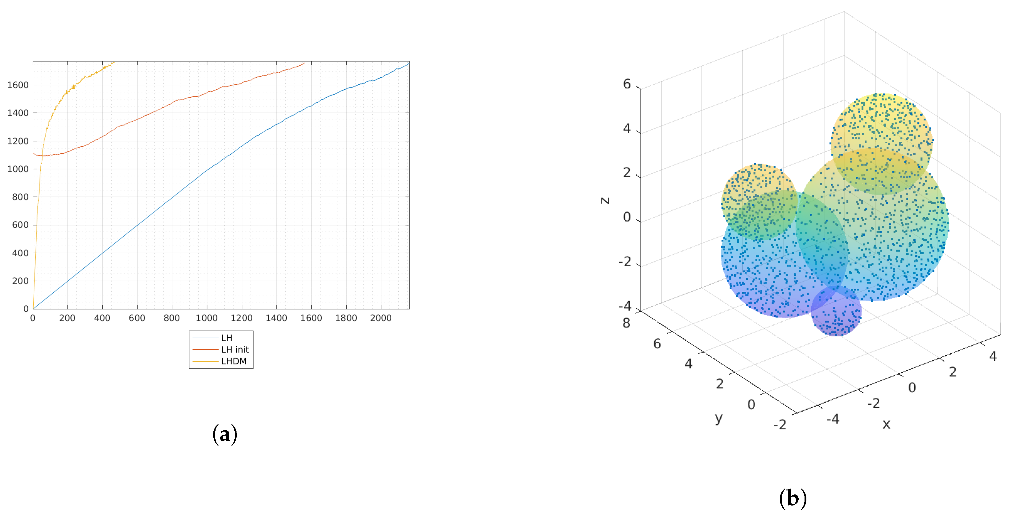
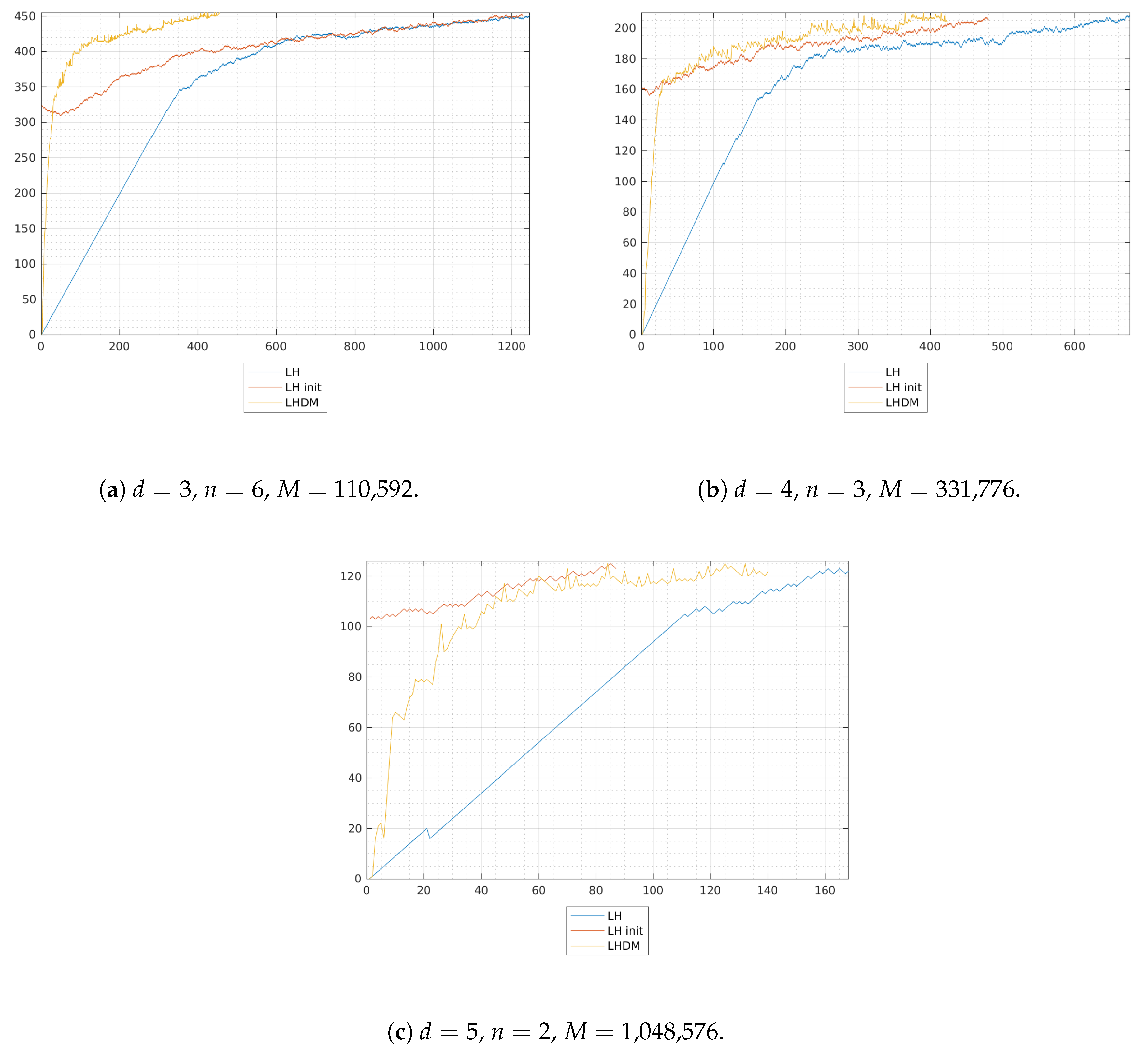
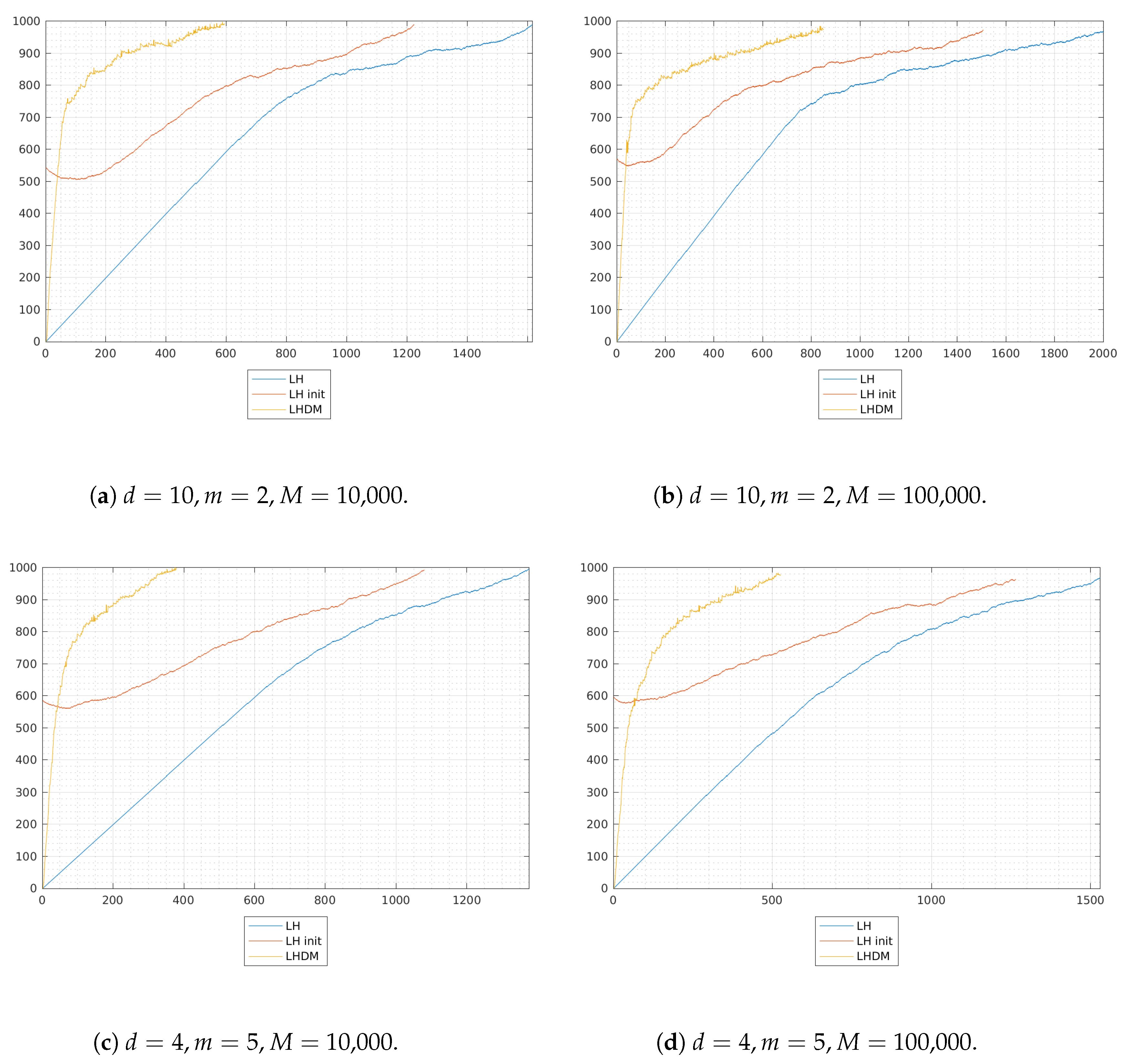
As a few examples of use cases of this package we have shown the results on a complex shape (multibubble) in three dimensions, and on hypercubes discretized with Chebyshev grids and with Halton points, testing different combinations of dimensions and degrees which generate large-scale problems for a personal computer.
The present package, dCATCH works for any discrete measure on a discrete set X. Indeed, it could be used, other than for design compression, also in the compression of d-variate quadrature formulas, even on lower-dimensional manifolds, to give an example.
We may observe that with this approach we can compute a d-variate compressed design starting from a high-cardinality sampling set X, that discretizes a continuous compact set (see Section 4.2 and Section 4.3). This design allows an m-th degree near optimal polynomial regression of a function on the whole X, by sampling on a small design support. We stress that the compressed design is function-independent and thus can be constructed “once and for all” in a pre-processing stage. This approach is potentially useful, for example, for the solution of d-variate parameter estimation problems, where we may think to model a nonlinear cost function by near optimal polynomial regression on a discrete d-variate parameter space X; cf., for example, References [32,33] for instances of parameter estimation problems from mechatronics applications (Digital Twins of controlled systems) and references on the subject. Minimization of the polynomial model could then be accomplished by popular methods developed in the growing research field of Polynomial Optimization, such as Lasserre’s SOS (Sum of Squares) and measure-based hierarchies, and other recent methods; cf., for example, References [34,35,36] with the references therein.
From a computational viewpoint, the results shown in Table 3, Table 4 and Table 5 show relevant speed-ups in the compression stage, with respect to the standard Lawson-Hanson algorithm, in terms of the number of iterations required and of computing time within the Matlab scripting language. In order to further decrease the execution times and to allow us to tackle larger design problems, we would like in the near future to enrich the package dCATCH with an efficient C implementation of its algorithms and, possibly, a CUDA acceleration on GPUs.

Author Contributions

Investigation, M.D., F.M. and M.V. All authors have read and agreed to the published version of the manuscript.

Funding

Work partially supported by the DOR funds and the biennial project Project BIRD192932 of the University of Padova, and by the GNCS-INdAM. This research has been accomplished within the RITA “Research ITalian network on Approximation”.

Conflicts of Interest

The authors declare no conflict of interest.

References

  1. Dessole, M.; Marcuzzi, F.; Vianello, M. dCATCH: A Numerical Package for Compressed d-Variate Near G-Optimal Regression. Available online: https://www.math.unipd.it/~marcov/MVsoft.html (accessed on 1 June 2020).
  2. Bos, L.; Vianello, M. CaTchDes: MATLAB codes for Caratheodory—Tchakaloff Near-Optimal Regression Designs. SoftwareX 2019, 10, 100349. [Google Scholar] [CrossRef]
  3. Dessole, M.; Marcuzzi, F.; Vianello, M. Accelerating the Lawson-Hanson NNLS solver for large-scale Tchakaloff regression designs. Dolomit. Res. Notes Approx. DRNA 2020, 13, 20–29. [Google Scholar]
  4. Atkinson, A.; Donev, A.; Tobias, R. Optimum Experimental Designs, with SAS; Oxford University Press: Oxford, UK, 2007. [Google Scholar]
  5. Pukelsheim, F. Optimal Design of Experiments; SIAM: Philadelphia, PA, USA, 2006. [Google Scholar]
  6. Celant, G.; Broniatowski, M. Interpolation and Extrapolation Optimal Designs 2-Finite Dimensional General Models; Wiley: Hoboken, NJ, USA, 2017. [Google Scholar]
  7. Mandal, A.; Wong, W.K.; Yu, Y. Algorithmic searches for optimal designs. In Handbook of Design and Analysis of Experiments; CRC Press: Boca Raton, FL, USA, 2015; pp. 755–783. [Google Scholar]
  8. De Castro, Y.; Gamboa, F.; Henrion, D.; Hess, R.; Lasserre, J.B. Approximate optimal designs for multivariate polynomial regression. Ann. Stat. 2019, 47, 127–155. [Google Scholar] [CrossRef] [Green Version]
  9. Dette, H.; Pepelyshev, A.; Zhigljavsky, A. Improving updating rules in multiplicative algorithms for computing D-optimal designs. Comput. Stat. Data Anal. 2008, 53, 312–320. [Google Scholar] [CrossRef] [Green Version]
  10. Torsney, B.; Martin-Martin, R. Multiplicative algorithms for computing optimum designs. J. Stat. Plan. Infer. 2009, 139, 3947–3961. [Google Scholar] [CrossRef]
  11. Bloom, T.; Bos, L.; Levenberg, N.; Waldron, S. On the Convergence of Optimal Measures. Constr. Approx. 2008, 32, 159–169. [Google Scholar] [CrossRef] [Green Version]
  12. Bos, L. Some remarks on the Fejér problem for lagrange interpolation in several variables. J. Approx. Theory 1990, 60, 133–140. [Google Scholar] [CrossRef] [Green Version]
  13. Calvi, J.P.; Levenberg, N. Uniform approximation by discrete least squares polynomials. J. Approx. Theory 2008, 152, 82–100. [Google Scholar] [CrossRef]
  14. Kiefer, J.; Wolfowitz, J. The equivalence of two extremum problems. Can. J. Math. 1960, 12, 363–366. [Google Scholar] [CrossRef]
  15. Putinar, M. A note on Tchakaloff’s theorem. Proc. Am. Math. Soc. 1997, 125, 2409–2414. [Google Scholar] [CrossRef]
  16. Titterington, D. Algorithms for computing D-optimal designs on a finite design space. In Proceedings of the 1976 Conference on Information Science and Systems; John Hopkins University: Baltimore, MD, USA, 1976; Volume 3, pp. 213–216. [Google Scholar]
  17. Burkardt, J. MONOMIAL: A Matlab Library for Multivariate Monomials. Available online: https://people.sc.fsu.edu/~jburkardt/m_src/monomial/monomial.html (accessed on 1 June 2020).
  18. Bos, L.; Piazzon, F.; Vianello, M. Near optimal polynomial regression on norming meshes. In Sampling Theory and Applications 2019; IEEE Xplore Digital Library: New York, NY, USA, 2019. [Google Scholar]
  19. Bos, L.; Piazzon, F.; Vianello, M. Near G-optimal Tchakaloff designs. Comput. Stat. 2020, 35, 803–819. [Google Scholar] [CrossRef]
  20. Tchakaloff, V. Formules de cubatures mécaniques à coefficients non négatifs. Bull. Sci. Math. 1957, 81, 123–134. [Google Scholar]
  21. Carathéodory, C. Über den Variabilitätsbereich der Fourier’schen Konstanten von positiven harmonischen Funktionen. Rendiconti Del Circolo Matematico di Palermo (1884–1940) 1911, 32, 193–217. [Google Scholar] [CrossRef] [Green Version]
  22. Sommariva, A.; Vianello, M. Compression of Multivariate Discrete Measures and Applications. Numer. Funct. Anal. Optim. 2015, 36, 1198–1223. [Google Scholar] [CrossRef] [Green Version]
  23. Pleśniak, W. Multivariate Jackson Inequality. J. Comput. Appl. Math. 2009, 233, 815–820. [Google Scholar] [CrossRef] [Green Version]
  24. Lawson, C.L.; Hanson, R.J. Solving Least Squares Problems; SIAM: Philadelphia, PA, USA, 1995; Volume 15. [Google Scholar]
  25. Van Benthem, M.H.; Keenan, M.R. Fast algorithm for the solution of large-scale non-negativity-constrained least squares problems. J. Chemom. 2004, 18, 441–450. [Google Scholar] [CrossRef]
  26. Hardin, D.; Michaels, T.; Saff, E. A Comparison of Popular Point Configurations on S2. Dolomit. Res. Notes Approx. DRNA 2016, 9, 16–49. [Google Scholar]
  27. Bloom, T.; Bos, L.; Calvi, J.; Levenberg, N. Polynomial Interpolation and Approximation in C d . Ann. Polon. Math. 2012, 106, 53–81. [Google Scholar] [CrossRef] [Green Version]
  28. De Marchi, S.; Piazzon, F.; Sommariva, A.; Vianello, M. Polynomial Meshes: Computation and Approximation. In Proceedings of the CMMSE 2015, Rota Cadiz, Spain, 6–10 July 2015; pp. 414–425. [Google Scholar]
  29. Dick, J.; Pillichshammer, F. Digital Nets and Sequences-Discrepancy Theory and Quasi—Monte Carlo Integration; Cambridge University Press: Cambridge, UK, 2010. [Google Scholar]
  30. Golub, G.H.; Van Loan, C.F. Matrix Computations, 3rd ed.; Johns Hopkins University Press: Baltimore, MD, USA, 1996. [Google Scholar]
  31. Slawski, M. Nonnegative Least Squares: Comparison of Algorithms. Available online: https://sites.google.com/site/slawskimartin/code (accessed on 1 June 2020).
  32. Beghi, A.; Marcuzzi, F.; Martin, P.; Tinazzi, F.; Zigliotto, M. Virtual prototyping of embedded control software in mechatronic systems: A case study. Mechatronics 2017, 43, 99–111. [Google Scholar] [CrossRef]
  33. Beghi, A.; Marcuzzi, F.; Rampazzo, M. A Virtual Laboratory for the Prototyping of Cyber-Physical Systems. IFAC-PapersOnLine 2016, 49, 63–68. [Google Scholar] [CrossRef]
  34. Lasserre, J.B. The moment-SOS hierarchy. Proc. Int. Cong. Math. 2018, 4, 3791–3814. [Google Scholar]
  35. De Klerk, E.; Laurent, M. A survey of semidefinite programming approaches to the generalized problem of moments and their error analysis. In World Women in Mathematics 2018-Association for Women in Mathematics Series; Springer: Cham, Switzerland, 2019; Volume 20, pp. 17–56. [Google Scholar]
  36. Martinez, A.; Piazzon, F.; Sommariva, A.; Vianello, M. Quadrature-based polynomial optimization. Optim. Lett. 2020, 35, 803–819. [Google Scholar] [CrossRef]
Figure 1. Multibubble test case, regression degree m = 10 . (a) The evolution of the cardinality of the passive set P along the iterations of the three LH algorithms. (b) Multibubble with 1763 compressed Tchakaloff points, extracted from 18,915 original points.
Mathematics 08 01122 g001
Figure 2. The evolution of the cardinality of the passive set P along the iterations of the three LH algorithms for Chebyshev nodes’ tests.
Mathematics 08 01122 g002
Figure 3. The evolution of the cardinality of the passive set P along the iterations of the three LH algorithms for Halton points’ tests.
Mathematics 08 01122 g003
Table 1. List of acronyms.
LSLeast Squares
NNLSNon-Negative Least Squares
LHLawson-Hawson algorithm for NNLS
LHILawson-Hawson algorithm with unconstrained LS Initialization
LHDMLawson-Hawson algorithm with Deviation Maximization acceleration
Table 2. dCATCH package content.
dCATCHd-variate CAratheodory-TCHakaloff discrete measure compression
dCHEBVANDd-variate Chebyshev-Vandermonde matrix
dORTHVANDd-variate Vandermonde-like matrix in a weighted orthogonal polynomial basis
dNORDd-variate Near G-Optimal Regression Designs
LHDMLawson-Hawson algorithm with Deviation Maximization acceleration
Table 3. Results for the multibubble numerical test: c o m p r = M / m e a n ( c p t s ) is the mean compression ratio obtained by the three methods listed; t L H / t T i t t is the ratio between the execution time of LH and that of the Titterington algorithm; t L H / t L H D M ( t L H I / t L H D M ) is the ratio between the execution time of LH (LHI) and that of LHDM; c p t s is the number of compressed Tchakaloff points and m o m e r r is the final moment residual.
Test LHLHILHDM
mMcompr t LH / t Titt t LH / t LHDM cptsmomerr t LHI / t LHDM cptsmomerrcptsmomerr
1018,91511/140.0/12.7/11755 3.4 × 10 8 3.2/11758 3.2 × 10 8 1755 1.5 × 10 8
Table 4. Results of numerical tests on M = ( 2 k m ) d Chebyshev’s nodes, with k = 4 , with different dimensions and degrees: c o m p r = M / m e a n ( c p t s ) is the mean compression ratio obtained by the three methods listed; t L H / t T i t t is the ratio between the execution time of LH and that of Titterington algorithm; t L H / t L H D M ( t L H I / t L H D M ) is the ratio between the execution time of LH (LHI) and that of LHDM; c p t s is the number of compressed Tchakaloff points and m o m e r r is the final moment residual.
Test LHLHILHDM
dmMcompr t LH / t Titt t LH / t LHDM cptsmomerr t LHI / t LHDM cptsmomerrcptsmomerr
36110,592250/10.4/13.1/1450 5.0 × 10 7 3.5/1450 3.4 × 10 7 450 1.4 × 10 7
43331,7761607/10.2/12.0/1207 8.9 × 10 7 3.4/1205 9.8 × 10 7 207 7.9 × 10 7
521,048,5768571/10.1/11.4/1122 6.3 × 10 7 1.5/1123 3.6 × 10 7 122 3.3 × 10 7
Table 5. Results of numerical tests on Halton points: c o m p r = M / m e a n ( c p t s ) is the mean compression ratio obtained by the three methods listed; t L H / t T i t t is the ratio between the execution time of LH and that of Titterington algorithm; t L H / t L H D M ( t L H I / t L H D M ) is the ratio between the execution time of LH (LHI) and that of LHDM; c p t s is the number of compressed Tchakaloff points and m o m e r r is the final moment residual.
Test LHLHILHDM
dmMcompr t LH / t Titt t LH / t LHDM cptsmomerr t LHI / t LHDM cptsmomerrcptsmomerr
10210,00010/141.0/11.9/19901.1 × 10 8 1.9/19889.8 × 10 9 9909.4 × 10 9
102100,000103/16.0/13.1/19683.6 × 10 7 2.8/19732.7 × 10 7 9684.2 × 10 7
4510,00010/120.2/12.3/19979.7 × 10 9 2.4/19931.3 × 10 8 9972.1 × 10 9
45100,000103/12.0/13.8/19696.6 × 10 7 3.8/19646.3 × 10 7 9695.3 × 10 7

