Comparison of Supervised Classification Models on Textual Data


Department of Industrial Engineering & Management, Cheng Shiu University, Kaohsiung 83347, Taiwan
Mathematics 2020, 8(5), 851; https://doi.org/10.3390/math8050851
Submission received: 8 May 2020
/
Revised: 21 May 2020
/
Accepted: 21 May 2020
/
Published: 24 May 2020
(This article belongs to the Special Issue Advances in Mathematical Methods for Machine Learning Algorithms for Computer Aided Diagnostic Systems)
Abstract
:Text classification is an essential aspect in many applications, such as spam detection and sentiment analysis. With the growing number of textual documents and datasets generated through social media and news articles, an increasing number of machine learning methods are required for accurate textual classification. For this paper, a comprehensive evaluation of the performance of multiple supervised learning models, such as logistic regression (LR), decision trees (DT), support vector machine (SVM), AdaBoost (AB), random forest (RF), multinomial naive Bayes (NB), multilayer perceptrons (MLP), and gradient boosting (GB), was conducted to assess the efficiency and robustness, as well as limitations, of these models on the classification of textual data. SVM, LR, and MLP had better performance in general, with SVM being the best, while DT and AB had much lower accuracies amongst all the tested models. Further exploration on the use of different SVM kernels was performed, demonstrating the advantage of using linear kernels over polynomial, sigmoid, and radial basis function kernels for text classification. The effects of removing stop words on model performance was also investigated; DT performed better with stop words removed, while all other models were relatively unaffected by the presence or absence of stop words.
1. Introduction
Classification, the process of assigning categories to data according to their content, plays an essential role in data analysis and management. Many classification methods have been proposed, such as the multimodal content retrieval framework introduced by Pouli et al. that uses personalized relevance feedback techniques to retrieve multimedia content tailored to individual users’ preferences [1] and the various methods presented by Thai et al. that retrieve and categorize the enormous amount of web content data in social networks [2]. Text classification is one form of classification that determines the value of the data in text and organizes the text in a certain way to enable it to be easily evaluated. Text classification is important for categorizing online content, such as topic detection of online news articles and spam detection in emails. Many text classification methods exist, such as the extended stochastic complexity (ESC) stochastic decision list proposed by Li and Yamanishi that uses if-then-else rules to categorize text [3]. However, these methods require deep knowledge of the domain of the text, and, since text does not take on a precise structure, the task of analyzing and interpreting text is extremely complex without the use of machine learning approaches. With the influx of machine learning algorithms that automate text classification, the process of extracting knowledge from unstructured textual data has become more effortless and efficient.
Machine learning-based systems consist of 3 different types: supervised learning, unsupervised learning, and semi-supervised learning (a combination of supervised and unsupervised learning methods). Supervised learning is the the process of training a model on labeled data, whereas unsupervised learning involves unlabeled data. Text classification is often performed using supervised machine learning algorithms due to the large number of labeled text datasets that allow for learning input-output pairs [4]; the use of unsupervised learning algorithms in text classification is more complex and less common as the algorithms work by clustering the input data without any knowledge of their labels [5]. Text classification can be performed using many different supervised learning methods including boosting, logistic regression (LR), decision trees (DT), random forest (RF), and support vector machines (SVMs) (especially kernel SVMs) [6].
The purpose of this study was to provide an in-depth assessment of the performance of supervised learning models on text classification using the 20 Newsgroups dataset, a multi-class classification problem [7], and the Internet Movie Database (IMDb) Reviews dataset, a binary-class classification problem [8]. These two datasets were employed to compare the results of the performance of the models on multi-class classification versus binary-class classification, which most studies have not done before. Data pre-processing, model evaluation, and hyperparameter tuning, as well as model validation on 8 models: LR, DT, SVM, AdaBoost (AB), RF, naive Bayes (NB), multilayer perceptrons (MLP), and gradient boosting (GB), were performed using pipelines.
Previous studies have used the 20 Newsgroups dataset to assess the performance of multiple models and found that SVM had the best performance [9]. Rennie et al. compared the performance of NB and SVM on multi-class text classification and found that SVM outperformed NB by approximately 10% to 20 % [10], which is consistent with the results of this study, where SVM had 70.03% and NB had 60.62% accuracy on the 20 Newsgroups dataset. Other studies assessed the performance of multiple classifiers, SVM, multinomial NB, and K-nearest neighbors for sentiment analysis using the IMDb dataset and obtained the best results using SVMs with a combination of information gain [11]. When comparing multiple models, including NB, SVM, AB, and LR, on the IMDb reviews dataset, Gamal et al. observed that SVM and LR were efficient and yielded great performance [12].
As expected from the results of past research studies, in this study, SVM performed the best on both datasets. LR followed close behind, while DT had the worst performance amongst all models. Textual data is often linearly separable, so SVMs are anticipated to be the best models since they are wide margin classifiers that learn linear threshold functions [13]. Since the split criteria at the top levels of a DT creates a bias towards specific classes, which becomes more extreme with increasing dimensionality, DTs perform poorly in large dimensional feature spaces, such as those in text datasets [14,15]. The removal of stop words worked well to improve the performance of DTs, possibly due to the decrease in feature dimension, while other models performed relatively the same in the presence or absence of stop words. The ranking of model performance is the same for both datasets, indicating that the ranking of model performance is independent of the type of classification performed (binary vs. multi-class). All models performed significantly better on the IMDb dataset, suggesting that binary-class classification is easier than multi-class classification. Further experimentation on SVMs showed that linear kernels gave the best performance compared to polynomial, sigmoid, and radial basis function kernels. Hence, the results of this study suggest that supervised learning models that learn linear threshold functions, such as linear SVMs, are most suitable for textual data.
This paper is organized as follows: Section 2 gives an overview of the models that are used in this study, which includes brief descriptions of the 8 models and comparisons of computational complexity and usage. Section 3, Section 4 and Section 5 outline the setup of the study, the proposed approach, and the results, respectively. Finally, Section 6 provides a discussion of the results, limitations of the study, and future directions, while Section 7 delivers a conclusion on the implications of this study.
2. Literature Reviews
LR and SVM are both supervised learning algorithms that are commonly used to solve classification problems. Both are used widely in classification tasks, such as cancer detection [16]. Although LR and SVM, particularly linear SVM, generally perform comparably well, their differing objective functions allow SVM to perform better in comparison on less structured data, such as images and text [16]. LR incorporates a statistical approach to assign discrete labels to data-points and finds any decision boundary that separates classes using the following cost function [17]:
where N is the number of instances or data-points, is the label for data-point n, x is the matrix of instances, and w is the weight vector.
On the other hand, SVM uses a geometrical approach to find the best or widest margin that separates data-points of different classes using the following objective function [18]:
subject to the following constraint:
with being the bias. The other variables are as defined for LR. The decision boundary for SVM is given by:
with M being the margin between the decision boundary that needs to be maximized as follows:
Figure 1 shows an illustration of an SVM trained with instances from two classes (yellow and purple points) and the decision boundary line (a maximum-margin hyperplane) in orange and margins M in blue. Anything above the boundary has a label of 1, whereas anything below the boundary has a label of −1. Instances on the margin are called the support vectors.
DT classifiers construct human-interpretable trees for dividing the input data into regions that give the lowest misclassification cost [19]. For predicting integer class labels, the cost per region k, , is defined as:
where is the number of instances in region k, and is the most frequent label in region k.
Although DTs are not sensitive to outliers and are robust to unnormalized input values, they are unstable and easy to overfit [20]. Common fixes include pruning and the employment of random forests. RF classifiers incorporate decision trees, bootstrap aggregation, and feature sub-sampling to reduce the correlation in DTs, which, consequently, decreases the variance of the models and increases overall accuracy [21]. As such, it is anticipated that RF will have better predictive power than DT.
AB and GB are boosting methods that create strong learners by sequentially combining weak learners or bases [22]. AB is commonly used in conjunction with DTs for boosting the performance of DTs. AB is also utilized in face detection applications, such as the Viola–Jones face detection framework [23]. AB uses the exponential loss function , where y is the actual label, and is the prediction, to optimize the cost function as follows [22]:
where is the label for instance n, is the loss for this instance at the previous stage, is the weight that will be updated depending on whether the data-point is correctly classified, and is the weak learner that is added onto the model at stage t.
Instead of adding on weak learners for each iteration of model training as done in AB, GB fits the weak learners to the gradient of the cost. GB is useful when the data has few dimensions but does not scale well in high dimensional data [24].
NB models, specifically multinomial NB, have been successfully applied to many domains, such as text classification. It is relatively robust and easy to implement with its lack of tunable hyperparameters. NB uses the feature values of the data to calculate the posterior probability that a particular object belongs to a given class as follows [25]:
where c is the class, x is the data, is the prior probability of class c, is the likelihood of observing the data in class c, and is the evidence.
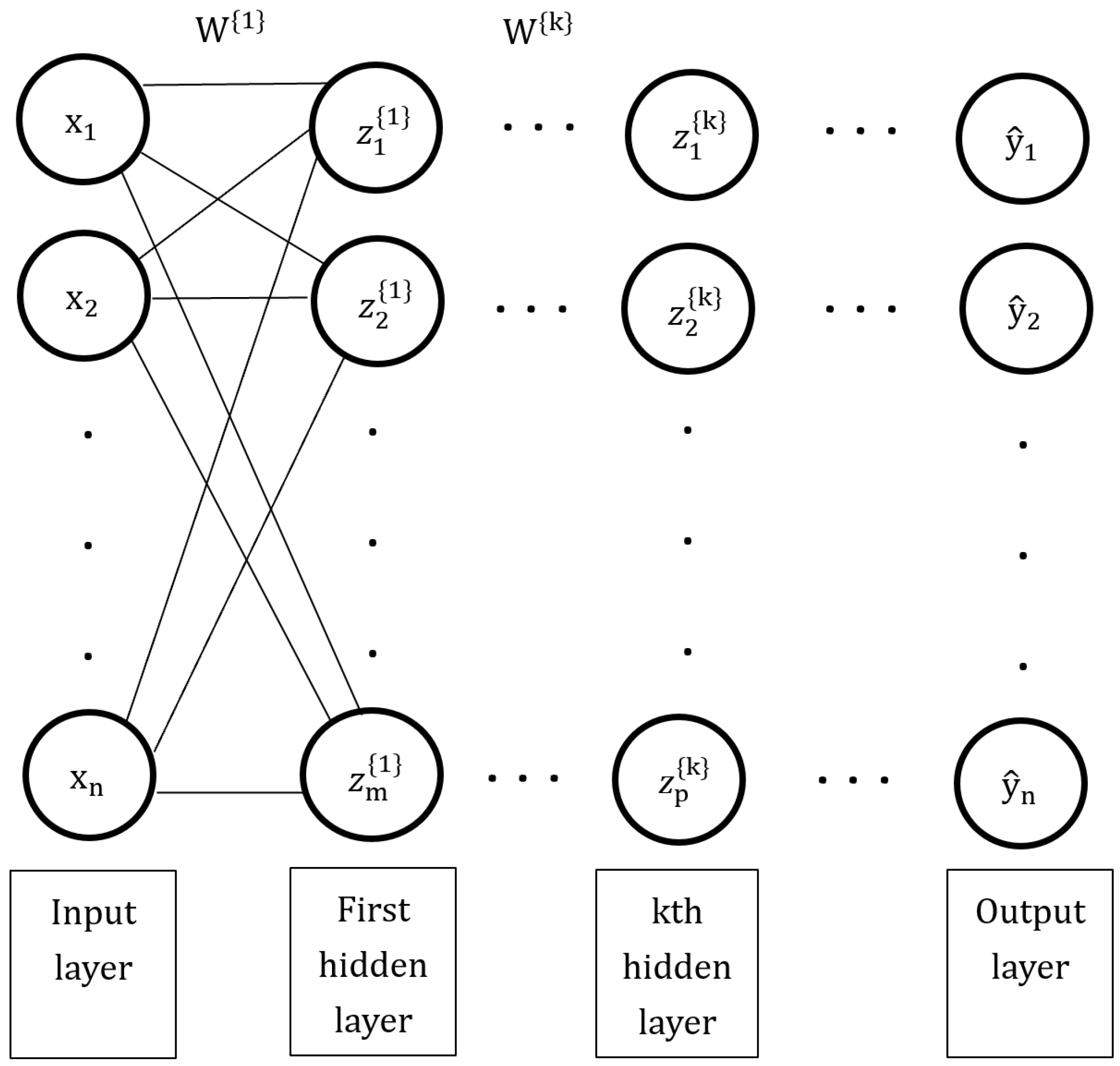
MLP models are classical types of neural networks that can be applied to any classification problem, such as image and text classification [26]. MLPs consist of an input layer, where data is fed in, one or more hidden layers, and an output layer, where predictions are made upon. An example of an MLP model is shown in Figure 2. The optimal weight vector () is found by taking the minimal W from the sum of the loss of each instance. The choice of the cost function L depends on the task. is the actual label, while is the prediction.
The output of one hidden layer () becomes the input to the next layer (). The nodes or neurons of the hidden layer(s) and output layer have non-linear activation functions (h) through which the nodes of the previous layer pass through [27].
Although the performance of a supervised machine learning algorithm is mainly measured by how well it approximates a function and performs the task of interest, the time and space complexity of a model is still useful when considering resource availability and model efficiency. Table 1 shows the theoretical time and space complexities of the 8 models used in this study compiled from various sources [28,29,30,31,32]. n is the number of samples, d is the input dimension (i.e., number of features) of a sample, c is the number of classes, t is the number of weak learners, f is the time complexity of each weak learner, is the number of trees used, is the number of support vectors, and k is the depth of the tree. Computational complexity is highly dependent on the implementation of the model, so complexity estimates often differ across studies. For instance, the MLP model’s space complexity varies depending on the number of hidden layers and hidden units in different layers, which is rarely consistent among different implementations [33]. Nevertheless, it is worthy of note that, although DT’s running time grows quadratically with the number of features in the input data, its space complexity is rather small and only depends on the height of the tree. Moreover, NB seems to be the least expensive in terms of both time and space due to its simplicity and its lack of hidden learning constants [30]. The scalability of the SVM to high dimensional feature spaces is demonstrated by the independence of its run-time and memory usage on the number of features in the data, as seen in Table 1, which allows the algorithm to perform equally well, in terms of computational complexity, on similar-sized samples regardless of feature dimension [29].
3. Dataset and Setup
The datasets used in this study are the 20 Newsgroups dataset retrieved from scikit-learn [7], consisting of 18,846 text samples and 20 classes and an IMDb Reviews dataset [8] containing 50,000 samples, with exactly half positive (rating of ≥ 7 out of 10) and half negative reviews (rating of ≤4 out of 10). Both datasets came with pre-split train and test sets. The data in both the train and test sets of the 20 Newsgroups dataset is unevenly split between each of the 20 classes. However, the class frequency rankings for the train and test sets are proportional and follow the same ranking order, with class 19 having the lowest frequency, and class 10 having the highest frequency (Figure 3).
Initial processing was performed on the IMDb dataset by removing any line breaks in each text file and merging the contents of individual data files together into a matrix. Data tokenization and transformation from occurrences to frequencies were performed on both datasets using the CountVectorizer and TfidfTransformer tools provided by the scikit-learn library [7]. Any punctuation within the data was ignored by CountVectorizer. After extracting the features, the 20 Newsgroups dataset had 101,631 features, while the IMDb dataset had 74,849. Additional pre-processing for removing stop words was performed.
4. Proposed Approach
A comparison of the performance of 8 classifiers, LR, DT, SVM, AB, RF, NB, MLP, and GB, was conducted using models and tools provided by scikit-learn [7].
Pipelines were constructed for each model, consisting of multiple steps, including feature extraction and pre-processing, term frequency–inverse document frequency (TFIDF) transformation, and model training using specified parameters. GridSearchCV from the scikit-learn library with 5-fold cross-validation was used to perform a search to select the best hyperparameter combinations from specified ranges of hyperparameters for each step in the pipeline. After this, the optimal hyperparameters found by GridSearchCV were used to re-train the model on the training set and to predict on the test set.
For model training, the accuracies yielded by the models on different ranges of hyperparameters were compared. For both LR and SVMs, both L1 and L2 regularization, different tolerance values for the stopping criteria, and various values for the inverse of regularization strength, C, were compared. Since regularization has a known role in reducing overfitting [34], these hyperparameters were chosen for tuning to discover the amount and type of regularization and early stopping criteria that are suitable for the classification tasks. The cost function was tuned for DT, using either Gini index or entropy, and for AB and GB, the number of estimators or weak learners was tuned, while, for RFs, both of these hyperparameters were tuned. The motivation behind selecting these hyperparameters stems from the fact that more weak learners help the model train better, but too many may cause it to overfit, with the exception of AB, which is slow to overfit [35]. Moreover, although Gini index and entropy have been shown to yield similar performance, it is still useful to see if they may differ in performance for binary and multi-class classification. Hyperparameters for MLP include the number and dimensions of the hidden layers, as well as the activation function. Experimentation on the use of different kernel bases for SVMs was also conducted. The effects of removing different lists of stop words on model performance was tested using the list of built-in English stop words in CountVectorizer [36] and the 179 stop words provided by the Natural Language Toolkit (NLTK) [37].
5. Results
Table 2 shows the best test accuracies yielded by all 8 models on the two datasets using the best hyperparameters outputted by GridSearchCV. Hyperparameters that are not in this table were set to the default values. The overall accuracy, which was computed by concatenating the predictions from both datasets and then comparing with the concatenation of the targets, estimates the overall performance of the models on the two datasets. To better visualize the performance of these models the test accuracy values of 5 selected models were plotted, as seen in Figure 4.
All 8 models performed better on the IMDb dataset than the 20 Newsgroups dataset (Table 2 and Figure 4). This may be due to the large size and even ratio of classes of the IMDb dataset. The 20 Newsgroups dataset has far fewer samples, 18,846, compared to the 50,000 samples in the IMDb dataset, and does not have equal class proportions. Furthermore, the IMDb dataset presents a binary classification problem, whereas the 20 Newsgroups dataset is a multi-class classification (20 classes) problem. Imbalanced datasets are more difficult to train and predict on [38], so combined with the fact that binary classification is typically less complex than multi-class classification, it is expected that the 8 models would perform better on the IMDB dataset. SVMs had the best performance for both datasets with an overall accuracy of 84.09%, and LR was not far behind with 83.63%, as seen in both Table 2 and Figure 4. Since LR and SVMs are similar in that they that both minimize an objective function consisting of a loss and penalty function [39], it is logical that they would give similar performance. Moreover, since most text categorization tasks are linearly separable and the SVM model learns linear threshold functions, SVMs are ideal classifiers for text classification [13]. SVMs also have the ability to generalize well even in the presence of many features [40], which is another favorable trait for text categorization since textual data is often high-dimensional. On the other hand, decision trees yielded the worst performance, with only 64.84% overall accuracy on both datasets. DTs suffer badly in high dimensional feature spaces, such as those in text datasets [14], so it is no surprise that it would have the worst accuracy amongst all the tested models. Although the RF classifier also incorporates decision trees, it performed much better than decision trees, possibly due to its feature subsampling procedure, which reduces the correlation between decision trees [14]. NB, MLP, and GB also performed quite well, as seen in Table 2. Although not as great as LR and SVMs, MLPs, which are commonly used in classification tasks [41], had the third highest overall test accuracy amongst all 8 models.
5.1. Testing Different Kernels for SVMs
Additionally, different types of kernels for SVMs were explored. According to scientific literature, textual data tends to be linearly separable [13], so it was expected that the linear kernel would yield a higher cross validation accuracy than the other kernels. This hypothesis was tested with 4 different types of kernels: linear, gaussian, polynomial, and sigmoid. Five-fold cross validation was performed to estimate the test accuracies of the different kernels.
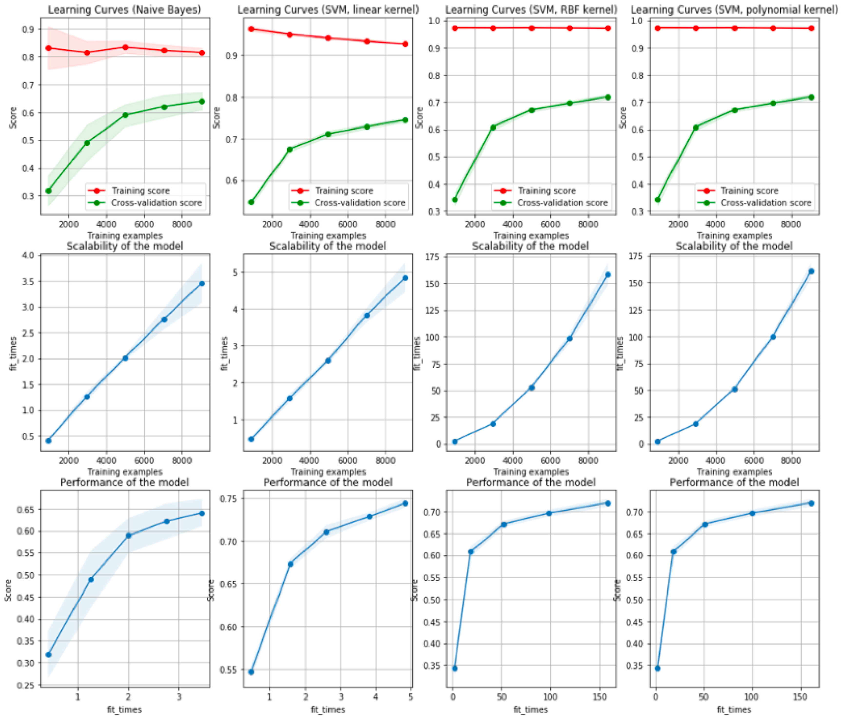
Table 3 shows that the linear SVM had the highest prediction accuracy out of all the different kernels. The 5-fold cross validation accuracy was 74.81% compared to 71.88% for the gaussian kernel, 65.81% for the sigmoid kernel, and 62.44% for the polynomial kernel. All of the SVM models were overfitting the training set, with the polynomial kernel overfitting the most as shown by the very high training accuracy compared to the relatively low cross validation accuracy in Figure 5. Indeed, the cross-validation and training accuracies do not seem to converge to the same value for all the models despite observing that the linear kernel performs the best [42]. As a result, GridSearchCV was used to obtain the optimal regularization hyperparameter in hopes of improving the accuracy. As seen in Figure 5, the training times of the linear SVM and the naive Bayes are linear with respect to the training set size. Furthermore, the maximum training time for the linear SVM is 5 s, which is very similar to 3.5 s for the naive Bayes model. On the other hand, for both non-linear kernel SVMs, the training time seems to scale exponentially with the training set size, and the maximum training time is around 160 s for both. This indicates that the linear SVM scales much better to large datasets than non-linear SVMs, and, since it has the highest cross-validation accuracy, it is the most desirable kernel for textual classification.
5.2. ROC Curves
Multi-class one-vs-all ROC curves for the 20 Newsgroups dataset were plotted using the predictions from 5 selected models with tuned parameters (Figure 6). Each class has its own ROC curve. From these plots, it can be seen that Class 10 has the highest area under the curve (AUC) for all 5 models, meaning that the models consistently have better prediction power for this class. Class 10 has the highest number of instances, as shown in Figure 3, which inherently allows for better classification, while, on the other hand, Class 19 has the lowest number of instances, thus having the lowest AUC for all 5 of the selected models.
ROC curves for the IMDb dataset using the output probabilities from each of the 8 models were plotted (Figure 7). As seen in the plots, LR and SVM give the highest AUC of 95%, which is reasonable as they also give the highest accuracies on the test set.
5.3. Tuning Hyperparameters
L2 regularization is the classic solution to the problem of estimating a classification problem with more features than observations [43]. Both of the datasets used in this study have a significantly larger number of features than instances, so the incorporation of L2 regularization into LR and SVM allowed for better model performance. While tuning the inverse of regularization strength parameter (C) for LR and SVM, LR required a larger C, i.e., less regularization, than SVMs for optimal performance as shown in Table 1. For both LR and SVM, the tolerance criteria for early stopping did not make a difference in the performance of the models, as shown in Figure 8a,c, where GridSearchCV results showed that model performance was the same for different values of the stopping criteria.
Both DT and RF models performed better using the Gini index cost function for the 20 Newsgroups dataset and using the entropy cost function for the IMDb dataset. This difference in performance was not as large for the IMDb dataset, with variations of less than , while, for the 20 Newsgroups dataset, there was a clear difference in performance between using Gini index and entropy as the cost function, as can be seen in Figure 8b,e. The number of estimators used in AB and RF is critical for optimal performance, as too few weak learners causes the models to underfit and too many leads to overfitting [35], which is demonstrated by the results in Figure 8d,e.
For DT in particular, there was a increase in the test accuracy of the model on the 20 Newsgroups dataset when stop words provided by CountVectorizer were removed, and a increase for the IMDb dataset when the NLTK stop words list was used, while all other models yielded relatively the same accuracies with or without removing stop words.
6. Discussion
There is no precise method for hyperparameter tuning; however, choosing hyperparameters that are relevant to the specifications of a model is still essential for achieving optimal model performance. Suggestions for hyperparameter selection include using regularization to reduce overfitting for models, such as LR and SVM, adding more or less weak learners for AB, RF, and GB classifiers to improve model performance or reduce overfitting, respectively, and changing the activation functions and the number and dimension of hidden layers for MLP.
This research presents some limitations that may be sources of further investigation. The optimization technique used for finding optimal hyperparameters, GridSearchCV, is vastly time-consuming, as it runs through every possible combination of hyperparameters, which may hinder those with limited computational power and time from replicating this study. A possible fix for this problem would be to implement an alternative optimization technique, such as scikit-learn’s RandomizedSearchCV [7], which tests a broader range of values within the same computation time as GridSearchCV, although optimality is not guaranteed. Another limitation is the high dimensionality of text when it is tokenized, which leads to expensive time and memory consumption and renders models that perform poorly in high dimensional feature spaces useless. To address this issue, dimensionality reduction methods, such as principal component analysis (PCA), can be incorporated to allow for faster computation and more accurate modeling [6].
Future directions could also involve performing different classification tasks on the datasets. The IMDb Reviews dataset used for this study also includes an unsupervised set where the reviews of any rating (1–10) are included. Thus, classification of the dataset could possibly be expanded to multi-class classification by adding a neutral class (rating of 5–6), as there may be reviews that are neither positive nor negative. Furthermore, multi-class classification could be done on the ratings (1–10) where each rating represents a class, instead of on the sentiment category (positive, negative). However, the accuracies for multi-class classification may be lower than the accuracies obtained for binary-class classification as there would be less instances for each class. On the other hand, for the 20 Newsgroups dataset, a possible extension would be to group the instances into more general classes so that classification can be done on less classes to assess potential improvement in model performance. Moreover, increasing the size of each of the two datasets by adding new instances may also improve performance.
7. Conclusions
The investigation of eight supervised learning models on text classification datasets demonstrated the dependence of model performance on not only the dataset size but also the proportionality of classes. An imbalanced number of instances per class causes the model to perform better (achieve a higher accuracy) on the classes with more instances. Moreover, models that generalize well on larger dimensional feature spaces, such as SVMs, have better predictive power in text classification than those that scale poorly in high feature dimensions. Another reason behind the success of SVMs in text classification is the independence of its computational complexity on the feature dimensions of the input data. Unlike other models in which time and/or space complexity are subject to the curse of dimensionality that comes with large feature spaces [44], SVMs are capable of performing equally well computationally on similar-sized data regardless of feature dimensions. Additionally, the use of linear kernels in SVMs is desirable for text classification because they are faster than other kernels and yield the best performance due to the linear separability of text datasets.
Although the unstructured nature of text makes it difficult to recognize and extract important details from it, by leveraging machine learning algorithms for text classification, we can structure messy documents into valuable information. The application of suitable machine learning models in text classification is critical for enabling the automation of online content and tasks, such as content tagging, spam detection, and efficient monitoring of social media. Pre-trained models on the IMDb dataset can be used for sentiment analysis research on social media, while those of the 20 Newsgroups dataset can be used to categorize online newspapers (topic detection) based on their content. Furthermore, automatic text classification creates potential for businesses related to rapid decision-making to identify critical information and provide real-time analysis and actions. With these applications of text classifiers in modern day tasks, jobs that were originally time-consuming and expensive can now be done efficiently and cost-effectively.
Funding
This research received no external funding.
Conflicts of Interest
The author declares no conflict of interest.
References
- Pouli, V.; Kafetzoglou, S.; Tsiropoulou, E.E.; Dimitriou, A.; Papavassiliou, S. Personalized multimedia content retrieval through relevance feedback techniques for enhanced user experience. In Proceedings of the 2015 13th International Conference on Telecommunications (ConTEL), Graz, Austria, 13–15 July 2015. [Google Scholar]
- Thai, M.T.; Wu, W.; Xiong, H. Big Data in Complex and Social Networks, 1st ed.; Chapman & Hall/CRC: Boca Raton, FL, USA, 2016. [Google Scholar]
- Li, H.; Yamanishi, K. Text classification using ESC-based stochastic decision lists. Inf. Process. Manag. 2002, 38, 343–361. [Google Scholar] [CrossRef]
- Kadhim, A.I. Survey on supervised machine learning techniques for automatic text classification. Artif. Intell. Rev. 2019, 52, 273–292. [Google Scholar] [CrossRef]
- Ko, Y.; Seo, J. Automatic text categorization by unsupervised learning. In Proceedings of the 18th conference on Computational linguistics—Volume 1, Saarbrücken, Germany, 31 July–4 August 2000; Volume 1, pp. 453–459. [Google Scholar]
- Kowsari, K.; Meimandi, K.J.; Heidarysafa, M.; Mendu, S.; Barnes, L.E.; Brown, D.E. Text Classification Algorithms: A Survey. Information 2019, 10, 150. [Google Scholar] [CrossRef] [Green Version]
- Pedregosa, F.; Varoquaux, G.; Gramfort, A.; Michel, V.; Thirion, B.; Grisel, O.; Blondel, M.; Prettenhofer, P.; Weiss, R.; Dubourg, V.; et al. Scikit-learn: Machine Learning in Python. J. Mach. Learn. Res. 2011, 12, 2825–2830. [Google Scholar]
- Maas, A.L.; Daly, R.E.; Pham, P.T.; Huang, D.; Ng, A.Y.; Potts, C. Learning Word Vectors for Sentiment Analysis. In Proceedings of the 49th Annual Meeting of the Association for Computational Linguistics: Human Language Technologies, Portland, OR, USA, 19–24 June 2011; pp. 142–150. [Google Scholar]
- Pradhan, L.; Taneja, N.A.; Dixit, C.; Suhag, M. Comparison of Text Classifiers on News Articles. Int. Res. J. Eng. Technol. (IRJET) 2017, 4, 2513–2517. [Google Scholar]
- Rennie, J.D.M.; Rifkin, R. Improving Multiclass Text Classification with the Support Vector Machine; Technical Report; MIT Aritificial Intelligence Laboratory: Cambridge, MA, USA, 2001. [Google Scholar]
- Ghosh, M.; Sanyal, G. Performance Assessment of Multiple Classifiers Based on Ensemble Feature Selection Scheme for Sentiment Analysis. Appl. Comput. Intell. Soft Comput. 2018, 2018. [Google Scholar] [CrossRef] [Green Version]
- Gamal, D.; Alfonse, M.; El-Horbarty, E.; M.Salem, A. Analysis of Machine Learning Algorithms for Opinion Mining in Different Domains. Mach. Learn. Knowl. Extr. 2019, 1, 224–234. [Google Scholar] [CrossRef] [Green Version]
- Joachims, T. Text Categorization with Support Vector Machines: Learning with Many Relevant Features. In Proceedings of the European Conference on Machine Learning, Chemnitz, Germany, 21–23 April 1998. [Google Scholar]
- Do, T.N.; Lenca, P.; Lallich, S.; Pham, N.K. Classifying Very-High-Dimensional Data with Random Forests of Oblique Decision Trees. In Advances in Knowledge Discovery and Management; Springer: Berlin/Heidelberg, Germany, 2010; pp. 39–55. [Google Scholar]
- Aggarwal, C.C. Machine Learning for Text; Springer: Berlin/Heidelberg, Germany, 2018. [Google Scholar]
- Salazar, D.A.; Velez, J.I.; Salazar, J.C. Comparison between SVM and Logistic Regression: Which One is Better to Discriminate? Rev. Colomb. Estadística 2012, 35, 223–237. [Google Scholar]
- Sperandei, S. Understanding logistic regression analysis. Biochem. Med. 2014, 24, 12–18. [Google Scholar] [CrossRef]
- Yue, S.; Li, P.; Hao, P. SVM classification: Its contents and challenges. Appl. Math. J. Chin. Univ. 2003, 18, 332–342. [Google Scholar] [CrossRef]
- Kotsiantis, S.B. Decision trees: A recent overview. Artif. Intell. Rev. 2013, 39, 261–283. [Google Scholar] [CrossRef]
- Kamiński, B.; Jakubczyk, M.; Szufel, P. A framework for sensitivity analysis of decision trees. Cent. Eur. J. Oper. Res. 2017, 26, 135–159. [Google Scholar] [CrossRef] [PubMed]
- Ho, T.K. The Random Subspace Method for Constructing Decision Forests. IEEE Trans. Pattern Anal. Mach. Intell. 1998, 20, 832–844. [Google Scholar]
- Wang, R. AdaBoost for Feature Selection, Classification and Its Relation with SVM, A Review. Phys. Procedia 2012, 25, 800–807. [Google Scholar] [CrossRef] [Green Version]
- Papageorgiou, C.; Oren, M.; Poggio, T. A General Framework for Object Detection. In Proceedings of the Sixth International Conference on Computer Vision, Chemnitz, Germany, 21–23 April 1998; Volume 6, pp. 555–562. [Google Scholar]
- Boehmke, B.; Greenwell, B. Hands-On Machine Learning with R; Chapman & Hall: Boca Raton, FL, USA, 2019. [Google Scholar]
- Russell, S.; Norvig, P. Artificial Intelligence: A Modern Approach, 2nd ed.; Prentice Hall: Upper Saddle River, NJ, USA, 2003. [Google Scholar]
- Wasserman, P.D.; Schwartz, T. Neural networks. II. What are they and why is everybody so interested in them now? IEEE Expert 1988, 3, 10–15. [Google Scholar] [CrossRef]
- Rosenblatt, F. Principles of Neurodynamics: Perceptrons and the Theory of Brain Mechanisms; Spartan Books: Torino, Italy, 1961. [Google Scholar]
- Su, J.; Zhang, H. A fast decision tree learning algorithm. In Proceedings of the 21st National Conference on Artificial Intelligence, Boston, MA, USA, 16–20 July 2006; Volume 1, pp. 500–505. [Google Scholar]
- Bottou, L.; Lin, C.J. Support Vector Machine Solvers. In Large-Scale Kernel Machines; Bottou, L., Chapelle, O., DeCoste, D., Weston, J., Eds.; MIT Press: Cambridge, MA, USA, 2007; pp. 301–320. [Google Scholar]
- Chu, C.; Kim, S.K.; Lin, Y.; Yu, Y.; Bradski, G.; Ng, A.Y.; Olukotun, K. Map-Reduce for Machine Learning on Multicore. Adv. Neural Inf. Process. Syst. 2006, 19, 281–288. [Google Scholar]
- Feng, W.; Huang, W.; Ren, J. Class Imbalance Ensemble Learning Based on the Margin Theory. Appl. Sci. 2018, 8, 815. [Google Scholar] [CrossRef] [Green Version]
- Natekin, A.; Knoll, A. Gradient boosting machines, a tutorial. Front. Neurorobotics 2013, 7, 21. [Google Scholar] [CrossRef] [Green Version]
- Serpen, G.; Gao, Z. Complexity Analysis of Multilayer Perceptron Neural Network Embedded into a Wireless Sensor Network. Procedia Comput. Sci. 2014, 36, 192–197. [Google Scholar] [CrossRef] [Green Version]
- Druck, G.; Mann, G.; McCallum, A. Learning from Labeled Features using Generalized Expectation Criteria. In Proceedings of the 31st Annual Iinternational ACM SIGIR Conference on Research and Development in Information Retrieval, Singapore, 20–24 July 2008; pp. 595–602. [Google Scholar]
- Wyner, A.J.; Olson, M.; Bleich, J.; Mease, D. Explaining the Success of Adaboost and Random Forests as Interpolating Classifiers. J. Mach. Learn. Res. 2017, 18, 1558–1590. [Google Scholar]
- Nothman, J.; Qin, H.; Yurchak, R. Stop Word Lists in Free Open-source Software Packages. In Proceedings of the Workshop for NLP Open Source Software (NLP-OSS), Melbourne, VIC, Australia, 15–20 July 2018; pp. 7–12. [Google Scholar]
- Bird, S.; Loper, E.; Klein, E. Natural Language Processing with Python; O’Reilly Media Inc.: Sebastopol, CA, USA, 2009. [Google Scholar]
- Adam, A.; Shapiai, M.I.; Chew, L.; Ibrahim, Z.; Jau, L.; Khalid, M.; Watada, J. A Two-Step Supervised Learning Artificial Neural Network for Imbalanced Dataset Problems. Int. J. Innov. Comput. Inf. Control (IJICIC) 2012, 8, 3163–3172. [Google Scholar]
- Zhang, J.; Jin, R.; Yang, Y.; Hauptmann, A. Modified Logistic Regression: An Approximation to SVM and Its Applications in Large-Scale Text Categorization. In Proceedings of the Twentieth International Conference on Machine Learning (ICML), Washington, DC, USA, 21–24 August 2003. [Google Scholar]
- Sun, A.; Lim, E.P.; Liu, Y. On strategies for imbalanced text classification using SVM: A comparative study. Decis. Support Syst. 2009, 48, 191–201. [Google Scholar] [CrossRef]
- Korde, V.; Mahender, C.N. Text Classification and Classifiers: A Survey. Int. J. Artif. Intell. Appl. (IJAIA) 2012, 3, 85–99. [Google Scholar]
- Wali, A. Clojure for Machine Learning; Packt Publishing: Birmingham, UK, 2014. [Google Scholar]
- Mazilu, S.; Iria, J. L1 vs. L2 Regularization in Text Classification when Learning from Labeled Features. In Proceedings of the 10th International Conference on Machine Learning and Applications and Workshops, Honolulu, HI, USA, 18–21 December 2011; pp. 166–171. [Google Scholar]
- Bellman, R.E. Adaptive Control Processes; Princeton University Press: Princeton, NJ, USA, 1961. [Google Scholar]
Figure 1.
Plot showing an support vector machine (SVM) trained with instances from two classes with its decision boundary and margins.
Figure 1.
Plot showing an support vector machine (SVM) trained with instances from two classes with its decision boundary and margins.

Figure 2.
Diagram showing an multilayer perceptrons (MLP) with its input layer ( to ), nodes (circles), hidden layers ( and ), and output layer ( to ). The bias term is omitted for simplicity.
Figure 2.
Diagram showing an multilayer perceptrons (MLP) with its input layer ( to ), nodes (circles), hidden layers ( and ), and output layer ( to ). The bias term is omitted for simplicity.

Figure 3.
Plots showing the class frequencies in the train and test sets of the 20 Newsgroup dataset.
Figure 3.
Plots showing the class frequencies in the train and test sets of the 20 Newsgroup dataset.

Figure 4.
Plot showing the best test accuracies yielded by 5 selected models on the two datasets using the best hyperparameters outputted by GridSearchCV.
Figure 4.
Plot showing the best test accuracies yielded by 5 selected models on the two datasets using the best hyperparameters outputted by GridSearchCV.

Figure 5.
Figure showing the learning curves for 4 different models: the multinomial naive Bayes and the linear, gaussian, and polynomial SVM models. This figure also shows the training time of the different model as a function of the training set size.
Figure 5.
Figure showing the learning curves for 4 different models: the multinomial naive Bayes and the linear, gaussian, and polynomial SVM models. This figure also shows the training time of the different model as a function of the training set size.

Figure 6.
ROC Curves for the 20 news groups of 5 models: logistic regression (LR), decision trees (DT), SVM, AdaBoost (AB), and random forest (RF).
Figure 6.
ROC Curves for the 20 news groups of 5 models: logistic regression (LR), decision trees (DT), SVM, AdaBoost (AB), and random forest (RF).

Figure 7.
ROC Curves for the 20 news groups of all 8 models.

Figure 8.
GridSearchCV (using 5-fold CV) results for hyperparameter tuning on the 5 models (LR, DT, SVM, AdaBoost, and RF) using the 20 Newsgroups dataset.
Figure 8.
GridSearchCV (using 5-fold CV) results for hyperparameter tuning on the 5 models (LR, DT, SVM, AdaBoost, and RF) using the 20 Newsgroups dataset.


Table 1.
Table showing the theoretical time and space complexity (in big O notation) of the 8 models used in this study.
Table 1.
Table showing the theoretical time and space complexity (in big O notation) of the 8 models used in this study.
| LR | DT | SVM | AB | RF | NB | MLP | GB | |
|---|---|---|---|---|---|---|---|---|
| Time Complexity | (nd2 + d3) | (nd2) | (n3) | (tf) | (n2dntrees) | (nd+dc) | (nd + dc) | (ndntrees) |
| Space Complexity | (d) | (k) | (nsv) | (nd) | (kntrees) | (dc) | Varies | (kntrees) |
Table 2.
Table showing the best test accuracies yielded by all 5 models on the two datasets using the best hyperparameters outputted by GridSearchCV. The best and worst test accuracies are highlighted in cyan and green, respectively.
Table 2.
Table showing the best test accuracies yielded by all 5 models on the two datasets using the best hyperparameters outputted by GridSearchCV. The best and worst test accuracies are highlighted in cyan and green, respectively.
| All Accuracies Are in Percentages and Rounded to 2 Decimal Places | LR | DT | SVM | AB | RF | NB | GB | MLP | |
|---|---|---|---|---|---|---|---|---|---|
| 20 News- groups | Best Test Accuracy | 68.28 | 44.44 | 70.03 | 45.61 | 62.28 | 60.62 | 60.12 | 69.46 |
| Best Hyper- parameters | Regularization: l2 C: 5.0 tol: 0.0001 | criterion: ’gini’ stopwords: sklearn | C: 0.3 tol: 1e-05 | n_estimators: 150 | criterion: ’gini’ n_estimators: 400 | N/A | loss: ’deviance’ learning_rate: 0.1 n_estimators: 200 | hidden_layer_sizes: (100, ) activation: ’relu’ | |
| IMDb Reviews | Best Test Accuracy | 88.28 | 71.64 | 88.32 | 84.63 | 84.84 | 83.02 | 83.56 | 86.04 |
| Best Hyper- parameters | Regularization: l2 C: 2.0 tol: 0.0001 | criterion: ’entropy’ stopwords: nltk | C: 0.4 tol: 1e-04 | n_estimators: 200 | n_estimators: 200 criterion: ’entropy’ | N/A | loss: ’deviance’ learning_rate: 0.1 n_estimators: 200 | hidden_layer_sizes: (100, ) activation: ’relu’ | |
| Overall | 83.63 | 64.84 | 84.09 | 75.59 | 79.62 | 77.83 | 77.13 | 82.20 | |
Table 3.
Table showing the cross validation and training accuracies yielded by all SVM models on the 20 Newsgroup dataset.
Table 3.
Table showing the cross validation and training accuracies yielded by all SVM models on the 20 Newsgroup dataset.
| Linear Kernel | Gaussian Kernel | Polynomial Kernel | Sigmoid Kernel | |
|---|---|---|---|---|
| Train Accuracy (%) | 92.08 ± 0.35 | 97.01 ± 0.64 | 97.20 ± 0.42 | 92.13 ± 0.13 |
| Test Accuracy (%) | 74.81 ± 0.64 | 71.88 ± 1.27 | 62.44 ± 0.76 | 65.81 ± 0.34 |
© 2020 by the author. Licensee MDPI, Basel, Switzerland. This article is an open access article distributed under the terms and conditions of the Creative Commons Attribution (CC BY) license (http://creativecommons.org/licenses/by/4.0/).
Share and Cite
MDPI and ACS Style
Hsu, B.-M. Comparison of Supervised Classification Models on Textual Data. Mathematics 2020, 8, 851. https://doi.org/10.3390/math8050851
AMA Style
Hsu B-M. Comparison of Supervised Classification Models on Textual Data. Mathematics. 2020; 8(5):851. https://doi.org/10.3390/math8050851
Chicago/Turabian StyleHsu, Bi-Min. 2020. "Comparison of Supervised Classification Models on Textual Data" Mathematics 8, no. 5: 851. https://doi.org/10.3390/math8050851
Note that from the first issue of 2016, this journal uses article numbers instead of page numbers. See further details here.