Article

Modified King’s Family for Multiple Zeros of Scalar Nonlinear Functions

1
Department of Mathematics, King Abdulaziz University, Jeddah 21589, Saudi Arabia
2
School of Mathematics, Thapar Institute of Engineering and Technology, Patiala 147004, India
3
DiGiES & Decisions Lab, University Mediterranea of Reggio Calabria, 89125 Reggio Calabria, Italy
*
Author to whom correspondence should be addressed.
These authors contributed equally to this work.
Mathematics 2020, 8(5), 827; https://doi.org/10.3390/math8050827
Submission received: 18 March 2020 / Revised: 26 April 2020 / Accepted: 12 May 2020 / Published: 19 May 2020
(This article belongs to the Special Issue Computational Methods in Analysis and Applications 2020)

Abstract

:
There is no doubt that there is plethora of optimal fourth-order iterative approaches available to estimate the simple zeros of nonlinear functions. We can extend these method/methods for multiple zeros but the main issue is to preserve the same convergence order. Therefore, numerous optimal and non-optimal modifications have been introduced in the literature to preserve the order of convergence. Such count of methods that can estimate the multiple zeros are limited in the scientific literature. With this point, a new optimal fourth-order scheme is presented for multiple zeros with known multiplicity. The proposed scheme is based on the weight function strategy involving functions in ratio. Moreover, the scheme is optimal as it satisfies the hypothesis of Kung–Traub conjecture. An exhaustive study of the convergence is shown to determine the fourth order of the methods under certain conditions. To demonstrate the validity and appropriateness for the proposed family, several numerical experiments have been performed. The numerical comparison highlights the effectiveness of scheme in terms of accuracy, stability, and CPU time.

1. Introduction

With the rapid growth of the numerical field, various physical and technical applications [1,2,3] are justifying the importance for solving the nonlinear equations. Such problems are arise in various fields of natural and physical sciences, including the heat and fluid flow problems, initial and boundary value problems, as well as problems associated with global positioning systems (GPS). For retrieving the solution through an analytical approach is almost inconceivable for any nonlinear equation except for some of them. Thus, iterative approaches provide an attractive alternative for solving these kinds of problems. While discussing about the root finding of nonlinear equation of the form f ( x ) = 0 , where f ( x ) is real function defined in a domain D R , we pictured the classical Newton’s method and for multiple roots, the modified Newton method [4,5,
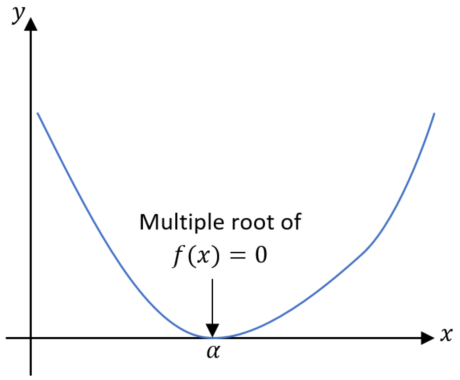
6] (also known as Rall’s method was introduced by E. Schröder in 1870) in mind. The modified Newton method is given by
x t + 1 = x t m f ( x t ) f ( x t ) .
Equation (1) converges quadratically for multiple roots with given multiplicity m 1 . Graphically, the sketch of multiple root is visualized from Figure 1. While, there are several one-point iterative approaches accessible in the literature, but they are not of practical relevance when presented from a real context, because of their theoretical shortcomings on convergence order and efficiency index. Moreover, most of the one-point approaches are computationally expensive and inefficient when evaluated on academic problems that arise from real life. Multipoint iterative approaches are therefore better choices to classify as appropriate solvers. One of the advantages of multipoint iterative methods without memory for scalar nonlinear equations is that we have a conjecture about their convergence order. For any multipoint method, requiring t functional evaluation can have atmost 2 t 1 convergence order, according to the hypothesis of Kung–Traub conjecture [5]. For instance, modified Newton method evaluating function at two points, and it reaches to the order 2 2 1 , for given m 1 . Hence, the modified Newton method is optimal in the sense of Kung–Traub Conjecture. Thus, a board community of researchers suggested several optimal [7,8,9,10,11,12,13,14,15,16,17,18,19] and non-optimal [20,21] multipoint iterative methods for estimating the multiple zeros of a function on the basis of Kung–Traub conjecture. For instance, Li et al. [9] investigated on the fourth-order scheme for calculating the multiple roots of an equation as follows:
y t = x t 2 m m + 2 f ( x t ) f ( x t ) , x t + 1 = x t b 1 f ( x t ) f ( x t ) f ( x t ) b 2 f ( x t ) + b 3 f ( y t ) ,
where b 1 = m m 2 2 , b 2 = 1 m , b 3 = 1 m m m + 2 m , where m denotes the multiplicity of the desired zero of given function f.
Sharma and Sharma [11] suggested the multipoint iterative method of order four, defined below:
y t = x t 2 m m + 2 f ( x t ) f ( x t ) , x t + 1 = x t a 1 w 1 ( x t ) a 2 w 2 ( x t ) a 3 w 2 2 ( x t ) w 1 ( x t ) ,
where w 1 ( x t ) = f ( x t ) f ( x t ) , w 2 ( x t ) = f ( x t ) f ( y t ) , a 1 = m 8 ( m 3 4 m + 8 ) , a 2 = 1 4 m m + 2 m + 1 ( m 1 ) ( m + 2 ) 3 , and a 3 = 1 8 ( m + 2 ) 4 m m + 2 2 m + 1 .
Moreover, Zhou et al. [12] developed the multipoint iterative method based on the weight function, and one of the particular form is:
y t = x t 2 m m + 2 f ( x t ) f ( x t ) , x t + 1 = x t m 8 [ m 3 m + 2 m 2 m f ( y t ) f ( x t ) 2 2 m 2 ( m + 3 ) m + 2 m m f ( y t ) f ( x t ) + ( m 3 + 6 m 2 + 8 m + 8 ) ] f ( x t ) f ( x t ) .
Recently, Behl and Hamdan [22] focused on the extension of Ostrowski’s methods for finding the multiple zeros, and given as:
y t = x t m f ( x t ) f ( x t ) , x t + 1 = x t m f ( x t ) f ( x t ) 1 u 1 2 u Q ( u ) ,
where u = f ( y t ) f ( x t ) 1 m and Q ( u ) is an weight function.
In literature, various researchers analyzed the variants of King’s family for solving the scalar nonlinear equation with multiplicity m = 1 . Recently, Behl and Hamdan [22] extended the Ostrowski’s method for multiple zero of a function. Whereas Sharma and Sharma [11] focused on the Jarratt’s method and modified it for computing the multiple roots. Till now for multiple zero function, the King’s family were not introduced in literature.
It is a challenging problem in the field of numerical analysis, to construct an optimal scheme of King’s family for approximating the multiple zero of a function. Thus, motivating from this idea, we have made an attempt to extend the King’s family [23] to optimal multipoint iterative method for obtaining the desire multiple zero of an input function. For this, we used the weight function technique. Furthermore, we have shown that the new method illustrates the good coordination with the numerical section, as it offers the smaller residual errors while estimating the multiple zeros of a function.
The manuscript is organized as follows: Section 2 first introduces the construction of new fourth-order scheme in general framework and then its theoretical analysis is provided. Moreover, in Section 3, several special cases are included, depending on the different weight functions used in the developed family. Whereas, Section 4 is confined to the numerical experiments that highlight the scheme’s effectiveness, accuracy, and stability on some intricate real-life problems. Section 5, presents the summary and conclusions.

2. Construction of the New Fourth-Order Multipoint Iterative Scheme

Consider the suggested iterative scheme as:
y t = x t m f ( x t ) f ( x t ) , x t + 1 = y t m f ( x t ) f ( x t ) 1 + β u t 1 + ( β 2 ) u t u t Q ( u t ) ,
where, β R , the weight function Q ( u t ) : C C is an analytic/holomorphic map [24,25] in the neighborhood of origin ( 0 ) with u t = f ( y t ) f ( x t ) 1 m . The u t is a multi-valued function. Considering the principal analytic branches of u t , as it is a multi-valued function. Moreover, it reduces the labour-period, by considering u t as a principal root known as u t = exp 1 m Log f ( y t ) f ( x t ) , with Log f ( y t ) f ( x t ) = Log f ( y t ) f ( x t ) + i Arg f ( y t ) f ( x t ) for π < Arg f ( y t ) f ( x t ) π , where A r g ( z ) is denotes the principal argument of z.
Without evaluating the new functional value, Theorem 1 shows that the proposed scheme converges with at least fourth-order of convergence. Moreover, the weight function is restricted under certain conditions and discussed in following theorem.
Theorem 1.
Consider the function f : D C C is an analytic inside the region D , enclosing the desired zero (say x = α m ) of the function f with the multiplicity m 1 . Then, the proposed strategy in Equation (6) attains the fourth-order of convergence provided it employ the following criteria:
Q ( 0 ) = 1 , Q ( 0 ) = 0 , | Q ( 0 ) | < .
Moreover, the following error expression is satisfied by the new scheme in Equation (6):
e t + 1 = 1 + 4 β + m Q ( 0 ) c 1 3 2 m c 1 c 2 2 m 3 e t 4 + O ( e t 5 ) ,
where error at t t h step e t = x t α m and c k = m ! ( m + k ) ! f ( m + k ) ( α m ) f ( m ) ( α m ) , k = 1 , 2 , 3 , 4 .
Proof. 
Let us assume that the scheme in Equation (6) has a multiple zero, x = α m with the known multiplicity m, greater than or equal to one. Expanding f ( x t ) and f ( x t ) about a point x = α m via the Taylor series expansion as follow:
f ( x t ) = f ( m ) ( α m ) m ! e t m 1 + i = 1 4 c i e t i + O ( e t 5 ) ,
and
f ( x t ) = f ( m ) ( α m ) ( m 1 ) ! e t m 1 1 + i = 1 4 m + i m c i e t i + O ( e t 5 ) ,
respectively.
Further, we have calculated the following expressions, with the use of Equations (9) and (10),
f ( x t ) f ( x t ) = 1 m e t c 1 m 2 e t 2 + ( 1 + m ) c 1 2 2 m c 2 m 3 e t 3 + O ( e t 4 ) ,
and
f ( y t ) = f x t m f ( x t ) f ( x t ) , = f ( m ) ( α m ) m ! c 1 m m e t 2 m 1 + 2 m c 2 ( m + 1 ) c 1 2 c 1 e t + ( m 3 + 3 m 2 + 3 m + 3 ) c 1 5 2 m ( 2 m 2 + 3 m + 2 ) c 1 3 c 2 + 4 m 2 ( m 1 ) c 1 c 2 2 + 6 m 2 c 1 2 c 3 2 m c 1 3 e t 2 + O ( e t 3 ) .
Using Equations (9) and (12), we obtain
u t = f ( y t ) f ( x t ) 1 m = c 1 m e t + 2 m c 2 ( m + 2 ) c 1 2 m 2 e t 2 + ( 2 m 2 + 7 m + 7 ) c 1 3 2 m ( 3 m + 7 ) c 1 c 2 + 6 m 2 c 3 2 m 3 e t 3 + O ( e t 4 ) .
and
1 + β u t 1 + ( β 2 ) u t u t = c 1 m e t c 1 2 2 c 2 m e t 2 + ( 2 m 2 m 4 β 1 ) c 1 3 + 2 m ( 1 3 m ) c 1 c 2 + 6 m 2 c 3 2 m 3 e t 3 + O ( e t 4 ) .
We conclude from Equation (13) that u t having linear order in e t . Therefore, expanding Q ( u t ) in the neighborhood of origin ( 0 ) as follow:
Q u t = Q ( 0 ) + u t Q ( 0 ) + 1 2 ! u t 2 Q ( 0 ) + 1 3 ! u t 3 Q ( 0 ) + O ( e t 4 ) = Q ( 0 ) + c 1 Q ( 0 ) m e t + c 1 2 ( Q ( 0 ) 2 ( m + 2 ) Q ( 0 ) ) + 4 c 2 m Q ( 0 ) 2 m 2 e t 2 + c 1 3 3 2 m 2 + 7 ( m + 1 ) Q ( 0 ) 6 ( m + 2 ) Q ( 0 ) + Q ( 0 ) 6 c 1 c 2 m ( ( 3 m + 7 ) Q ( 0 ) 2 Q ( 0 ) ) + 18 c 3 m 2 Q ( 0 ) 6 m 3 e t 3 + O ( e t 4 ) ,
by adopting Taylor series expansion.
By substituting Equations (11), (14) and (15) in the scheme in Equation (6), we have
e t + 1 = y t m f ( x t ) f ( x t ) 1 + β u t 1 + ( β 2 ) u t u t Q u t = ( 1 Q ( 0 ) ) c 1 m e t 2 + c 1 2 ( m ( Q ( 0 ) 1 ) + Q ( 0 ) Q ( 0 ) 1 ) 2 c 2 m ( Q ( 0 ) 1 ) m 2 e t 3 + 1 2 m 3 [ c 1 3 ( 2 m 2 ( Q ( 0 ) 1 ) + m ( 3 Q ( 0 ) 4 Q ( 0 ) 4 ) + ( 1 4 β ) Q ( 0 ) 6 Q ( 0 ) + Q ( 0 ) 2 ) 2 c 1 c 2 m ( 3 m ( Q ( 0 ) 1 ) + 3 Q ( 0 ) 4 Q ( 0 ) 4 ) + 6 c 3 m 2 ( Q ( 0 ) 1 ) ] e t 4 + O ( e t 5 ) .
For attaining the fourth-order of convergence by the presented method in Equation (6), the coefficients of terms e t 2 , and e t 3 should be zero at the same time. Thus, from Equation (16) the following system of equations is obtained that involve Q ( 0 ) , and its first derivative Q ( 0 ) :
1 Q ( 0 ) = 0 , Q ( 0 ) = 0 ,
which further yields the following restriction on weight function Q :
Q ( 0 ) = 1 , Q ( 0 ) = 0 .
By substituting Equation (18) in Equation (16), the following error equation and asymptotic constant is satisfied by scheme defined in Equation (6):
e t + 1 = 1 + 4 β + m Q ( 0 ) c 1 3 2 m c 1 c 2 2 m 3 e t 4 + O ( e t 5 ) ,
where | Q ( 0 ) | < .
Thus, the Equation (19) justifies that the presented family in Equation (6) reaches to the optimal convergence order by just evaluating the 3 functional ( f ( x ) , f ( y ) , and f ( x ) ) at each iterate. This completes the proof. □

3. Variants of New Family in Equation (6)

It is straightforward to have from Theorem that one can get modified strategies of King’s family by employing some particular values of Q ( u t ) and by introducing various forms of weight functions.
Case 1. Considering the following polynomial weight function:
Q ( u t ) = A u t 3 + 1 ,
where Q ( 0 ) = 6 A , where | A | < .
In view of Equation (20) and scheme in Equation (6), the new fourth-order optimal family is obtained as follows:
y t = x t m f ( x t ) f ( x t ) , x t + 1 = y t m f ( x t ) f ( x t ) 1 + β u t 1 + ( β 2 ) u t A u t 4 + u t .
Some of the sub-special cases for Equation (21)
(i) When β = 0 , and A = 0 , the proposed scheme in Equation (21) read as:
y t = x t m f ( x t ) f ( x t ) , x t + 1 = y t m f ( x t ) f ( x t ) 1 1 2 u t u t .
(ii) For β = 1 , and A = 1 2 , the family in Equation (21) becomes:
y t = x t m f ( x t ) f ( x t ) , x t + 1 = y t m 2 f ( x t ) f ( x t ) 1 u t 1 3 u t u t 4 + 2 u t .
The above Equation (23) is another particular case of the scheme in Equation (6).
Case 2. Choosing the rational weight function as defined below:
Q ( u t ) = 1 + A 1 u t + A 2 u t 2 1 + A 1 u t , provided A 1 u t 1 ,
and where Q ( 0 ) = 2 A 2 , here A 2 is any finite real number. Adopting the weight function in Equation (24) in the proposed scheme in Equation (6), we have
y t = x t m f ( x t ) f ( x t ) , x t + 1 = y t m f ( x t ) f ( x t ) 1 + β u t 1 + ( β 2 ) u t u t ( 1 + A 1 u t + A 2 u t 2 ) 1 + A 1 u t ,
which is another new type of multipoint family.
Some of the sub-special cases for Equation (25)
(i) For β = 1 2 , A 1 = 1 10 , and A 2 = 2 , the scheme in Equation (25) reads as
y t = x t m f ( x t ) f ( x t ) , x t + 1 = y t m f ( x t ) f ( x t ) u t ( u t + 2 ) ( 20 u t 2 + u t + 10 ) ( u t + 10 ) ( 3 u t 2 ) .
In this way, we obtain another particular form of fourth-order optimal iterative technique.
(ii) For β = 2 , A 1 = 6.45 , and A 2 = 10 , the family in Equation (25) leads us
y t = x t m f ( x t ) f ( x t ) , x t + 1 = y t m f ( x t ) f ( x t ) u t ( 400 u t 3 458 u t 2 + 89 u t + 20 ) 516 u t 2 + 49 u t + 20 ,
a new optimal 4th-order iterative scheme.
Case 3. Consider the another rational function that defines the weight function as:
Q ( u t ) = 1 + A 1 u t 1 + A 1 u t + A 2 u t 2 ,
where Q ( 0 ) = 2 A 2 , where A 2 is the finite real value.
By substituting Equation (28) in Equation (6), the new optimal family of 4th-order can obtained as follows:
y t = x t m f ( x t ) f ( x t ) , x t + 1 = y t m f ( x t ) f ( x t ) 1 + β u t 1 + ( β 2 ) u t u t ( 1 + A 1 u t ) 1 + A 1 u t + A 2 u t 2 .
Some of the sub-special cases for the scheme in Equation (29)
(i) For β = 1 4 , A 1 = 0 , and A 2 = 1 10 , the family in Equation (6) provides us the special case of Equation (29)
y t = x t m f ( x t ) f ( x t ) , x t + 1 = y t m f ( x t ) f ( x t ) 10 u t ( u t 4 ) ( 9 u t 4 ) ( u t 2 + 10 ) .
(ii) For β = 10 , A 1 = 4 , and A 2 = 21 , the family in Equation (29) read as
y t = x t m f ( x t ) f ( x t ) , x t + 1 = y t m f ( x t ) f ( x t ) u t ( 4 u t + 1 ) ( 10 u t + 1 ) ( 8 u t + 1 ) ( 21 u t 2 + 4 u t + 1 ) ,
is another new fourth-order optimal multipoint method.

4. Numerical Testing and Discussions

This section is aimed to confirm the theoretical aspects by numerical examination. For this, an attempt is made to demonstrate the comparison of the new approach to practical and academic structures with the existing strategies. For justifying the proposed scheme in Equation (6), we have compared our new schemes defined in Equation (26), and Equation (30) denoted by M M 1 , and M M 2 , and compared with the existing methods defined in Equations (2)–(4), denoted by L M , S M , and Z M , respectively. Moreover, the results are compared with the expression in Equation (5), (for equation number R M (32) of article [22]).
The numerical outcomes are displayed in Table 1, Table 2, Table 3, Table 4, Table 5 and Table 6, by comparing our techniques with existing methods in terms of approximate zeros ( x t ), absolute residual error of the considered function ( | f ( x t ) | ) , absolute difference in two successive approximations | x t + 1 x t | , computational order of convergence ρ log | f ( x t + 1 ) / f ( x t ) | log | f ( x t ) / f ( x t 1 ) | , t 2 , (see [26,27]), at the last iteration indices (t), and computational time ( T i m e ) in seconds. We have maintained 2000 significant digits of minimum precision to minimize the round off error.
As mentioned within the above description, we determine the value of all the functional residual and the constants till 2000 significant digits, however, we have displayed the value of obtained approximated zero of the function up-to twenty-five significant digits. Whereas, the absolute error in the successive approximations | x t + 1 x t | and the residual error | f ( x t ) | exhibited till two significant digits along with the exponent power. Moreover, the computational convergence order is shown up-to five digits. The results are obtained with the help of M a t h e m a t i c a software (version 11.1, Wolfram Research, Tokyo, Japan).
Note that for calculating the multiplicity m of a root, one may use the following ways:
(i) Traub in [5] proposed the following approximation formula that
m log | f ( x ) | log | f ( x ) / f ( x ) | ,
when x is very close to the multiple root of f.
(ii) Lagouanelle in [28] introduced the following expression:
m f ( x ) 2 f ( x ) 2 f ( x ) f ( x ) ,
where x is very close to the multiple root of f.
Example 1.
(Van der Waals equation of state):
Consider the following Van der Waals equation of state:
P + a ¯ n 2 V 2 ( V n b ¯ ) = n R T ,
where the parameter a ¯ and b ¯ (known as Van der Wall’s constants) depends upon critical temperature, and critical pressure of the specified gas. Evaluate V (volume of the gas) with respect to known values of remaining variables by calculating the solution of the following equation:
P V 3 ( n b ¯ P + n R T ) V 2 + a ¯ n 2 V a ¯ b ¯ n 2 = 0 .
Thus, the above equations have at least one real root, as it is cubic polynomial. By using the specific values of the parameters, the following nonlinear function of V = x is obtained:
f ( x ) = x 3 5.22 x 2 + 9.0825 x 5.2675 ,
having the three zeros: 1.72, 1.75, and 1.75. Thus, the required root is α = 1.75 (as multiplicity is two).
The numerical performance presented in Table 1 shows the better outcomes of the presented methods M M 1 , and M M 2 with respect to the precision in calculating the multiple root of f ( x ) = 0 , whereas, M M 2 is over-performing in terms of accuracy.
Example 2.
(Problem of Planck’s radiation law):
Now, consider the defined below problem of Planck’s radiation law which measures the spectral density of electromagnetic radiations released by a black-body at a given temperature, at thermal equilibrium [29] as:
Φ ( λ ) = 8 π h c λ 5 exp c h λ k B T 1 1 ,
where T , λ , k B , h , and c denotes the absolute temperature of the black-body, wavelength of radiation, Boltzmann constant, Plank’s constant, and speed of light in the medium (vacuum), respectively. We are interested to determine the wavelength λ which results to the maximum energy density Φ ( λ ) .
Further, the first derivative of Φ is equated to zero, which corresponds to the maximum value of Φ at:
c h λ k B T exp c h λ k B T exp c h λ k B T 1 = 5 .
If x = c h λ k B T , then Equation (33) is satisfied when
f ( x ) = 5 exp ( x ) + x 5 = 0 .
Thus, the solutions of Equation (34), results the maximum values of λ, and is means by the given below expression:
λ c h α k B T ,
where α is a solution of Equation (34). Our desired root is x = 4.9651142317442 with multiplicity m = 1 .
The numerical outcomes for Equation (34) are illustrated in Table 2. It can be declared by observing the results that the M M 1 and M M 2 methods have smaller residual errors in contrast to the existing methods when the accuracy of root is computed in multi-precision arithmetic. Moreover, the time consumed by new methods while computing the results is lesser with respect to other techniques, which justifying the attempt of developing the new scheme.
Example 3.
(Fractional conversion of a reactant in chemical reactor):
Considering the fractional conversion of a given species A (please, refer to [30] for further details of this problem) in terms of x as
f ( x ) = x x 1 + 5 log 0.4 0.5 x 0.4.1 x ) + 4.45977 .
If x > 0 or x < 1 , then there is no significant meaning of the above defined fractional conversion. Which indicates that the x is bounded in its complementary region i.e., 0 x 1 . Moreover, this problem is not defined for the x [ 0.8 , 1 ] , and this region is nearly to the required root α 0.757396246253753879459641297929 . Furthermore, this function has some other properties, which make the solution tougher to estimate. For instance, when x = 1.098 , the test problem has an infeasible solution, whereas its derivative is very close to zero for 0 x 0.5 .
The outcomes for this test function are determined in Table 3. Clearly, it indicates that the proposed scheme works faster than others with greater accuracy. Although, L I show higher accuracy but results with higher computational time, whereas our methods results earlier.
Example 4.
Continuous stirred tank reactor:
Consider the following sequence of reaction taken place in reactor (for further study, refer [31])
a + R b , b + R c , c + R d , d + R e
In the above sequence, the components a and R are supplied with the rate t and q t , respectively to the reactor. For draft of simple feedback from control system, Douglas [32] analyzed this problem in detail and introduced the following expression to study the transfer function of the reactor.
K c 2.98 ( x + 2.25 ) 4.35 + x ) ( 1.45 + x ) ( 2.85 + x ) 2 = 1 ,
where K c stands for the gain of the proportional controller. The control system is stable for values of K C that yields roots of the transfer function having negative real part. If we choose K C = 0 , we get the poles of the open-loop transfer function as roots of the nonlinear equation:
f ( x ) = x 4 + 11.50 x 3 + 47.49 x 2 + 83.06325 x + 51.23266875 ,
given as: x = 1.45 , 2.85 , 2.85 , 4.35 . Thus, one of root have multiplicity is equal to two. Hence, it is our desired root.
From Table 4, we can observe that the new methods M M 1 , M M 2 , and the existing R M method show equivalent accuracy of the desired result and resulting well with lesser residual error and difference in successive obtained approximations in comparison to the other considered methods. Along with this, numerical convergence order is justifying our theoretical analysis.
Example 5.
The characteristic polynomial of non-singular matrix
B = 29 14 2 6 9 47 22 1 11 13 19 10 5 4 8 19 10 3 2 8 7 4 3 1 3 ,
is defined as a function:
f ( x ) = ( x 2 ) 4 ( x + 1 ) .
Clearly, the characteristic function in Equation (40) has one of the zeros with multiplicity m = 4 . Thus, the desired root is α = 2 , while testing the schemes.
The numerical outcomes of the nonlinear function in Equation (40) depicts that the newly proposed schemes M M 1 and M M 2 have splendid outcomes in the view of less residual error and estimation of the convergence order. Moreover, the results are achieved faster than other techniques.
Example 6.
Consider the another nonlinear testing sample from [6], as follows:
f ( x ) = ( x c o s ( x ) ) 5 .
The above test function has one of the multiple zero at α = 0.739085133215161 with m = 5 .
The results of this test problem is shown in Table 6. We can observe from the numerical tests showed in this table that results by presented methods achieve are much effective in minimum time period than its competitors.
Example 7.
Kepler’s law of planetary motion says that a plant revolve around sun in a elliptic order. Assume that the point ( x , y ) defines the position of plant at time t, which can be evaluated by following expressions:
x = a cos ( E e ) ,
y = a 1 e 2 sin ( E ) ,
where E stands for eccentric anomaly and e stands for the eccentricity of the ellipse.
To determine the position ( x , y ) , we need to compute E, which can be calculated by the use of Kepler’s equation of motion:
M = E e sin ( E ) , 0 < e < 1 ,
where M is the mean anomaly. The above equation relates the mean anomaly M to the eccentric anomaly E of an elliptic orbit with eccentricity e. Thus to compute E, one can solve the following nonlinear function
f ( E ) = M E + e sin ( E ) .
For testing the various iterative methods, we consider M = 0.01 , e = 0.9995 , and initial approximation as M + e . The approximate zero of the function defined in above equation is α 0.3899777749463621 . The results are demonstrated in Table 7, which manifest that the proposed methods are winning in each aspects of comparisons.

5. Summary and Conclusions

The main remarks of the study are:
  • A new optimal variant of King’s family for finding the desired multiple zero of a given function is developed.
  • The presented multipoint iterative scheme uses function at two values and involves only the first derivative at one point of each iteration.
  • The structure of the scheme is dependent upon the weight function under certain conditions. With the aid of weight function, various fourth order schemes can be obtained.
  • A wide range of real-life applications is introduced in the numerical segment to validate the efficacy of the suggested modified family as compared to the alternative methods.
    (a)
    From the experimental outcomes, we can point out that the new tools provide superior results for the considered test functions in terms of precision and accuracy.
    (b)
    Moreover, the time used for evaluating the desired results by new methods indicates the effectiveness over the other techniques.

Author Contributions

All the authors have equal contribution. All authors have read and agreed to the published version of the manuscript.

Funding

This work is supported by the Deanship of Scientific Research (DSR), King Abdulaziz University, Jeddah, Saudi Arabia under the grant number D-539-130-1441.

Acknowledgments

The authors, therefore, gratefully acknowledge the DSR technical and financial support.

Conflicts of Interest

The authors declare no conflict of interest.

References

  1. Azarmanesh, M.; Dejam, M.; Azizian, P.; Yesiloz, G.; Mohamad, A.A.; Sanati-Nezhad, A. Passive microinjection within high-throughput microfluidics for controlled actuation of droplets and cells. Sci. Rep. 2019, 9, 1–12. [Google Scholar] [CrossRef] [PubMed]
  2. Dejam, M. Advective-diffusive-reactive solute transport due to non-Newtonian fluid flows in a fracture surrounded by a tight porous medium. Int. J. Heat Mass Transf. 2019, 128, 1307–1321. [Google Scholar] [CrossRef]
  3. Nikpoor, M.H.; Dejam, M.; Chen, Z.; Clarke, M. Chemical-Gravity-Thermal Diffusion Equilibrium in Two-Phase Non-isothermal Petroleum Reservoirs. Energy Fuel 2016, 30, 2021–2034. [Google Scholar] [CrossRef]
  4. Ostrowski, A.M. Solution of Equations and Systems of Equations; Academic Press: New York, NY, USA, 1960. [Google Scholar]
  5. Traub, J.F. Iterative Methods for the Solution of Equations; Prentice-Hall: Englewood Cliffs, NJ, USA, 1964. [Google Scholar]
  6. Petković, M.S.; Neta, B.; Petković, L.D.; Džunić, J. Multipoint Methods for Solving Nonlinear Equations; Academic Press: New York, NY, USA, 2013. [Google Scholar]
  7. Behl, R.; Cordero, A.; Motsa, S.S.; Torregrosa, J.R. On developing fourth-order optimal families of methods for multiple roots and their dynamics. Appl. Math. Comput. 2015, 265, 520–532. [Google Scholar] [CrossRef] [Green Version]
  8. Behl, R.; Cordero, A.; Motsa, S.S.; Torregrosa, J.R.; Kanwar, V. An optimal fourth-order family of methods for multiple roots and its dynamics. Numer. Algorithms 2016, 71, 775–796. [Google Scholar] [CrossRef]
  9. Li, S.; Liao, X.; Cheng, L. A new fourth-order iterative method for finding multiple roots of nonlinear equations. Appl. Math. Comput. 2009, 215, 1288–1292. [Google Scholar]
  10. Neta, B.; Chun, C.; Scott, M. On the development of iterative methods for multiple roots. Appl. Math. Comput. 2013, 224, 358–361. [Google Scholar] [CrossRef] [Green Version]
  11. Sharma, J.R.; Sharma, R. Modified Jarratt method for computing multiple roots. Appl. Math. Comput. 2010, 217, 878–881. [Google Scholar] [CrossRef]
  12. Zhou, X.; Chen, X.; Song, Y. Constructing higher-order methods for obtaining the multiple roots of nonlinear equations. J. Comput. Appl. Math. 2011, 235, 4199–4206. [Google Scholar] [CrossRef] [Green Version]
  13. Behl, R.; Salimi, M.; Ferrara, M.; Sharifi, S.; Samaher, K.A. Some real life applications of a newly constructed derivative free iterative scheme. Symmetry 2019, 11, 239. [Google Scholar] [CrossRef] [Green Version]
  14. Behl, R.; Alsolami, A.J.; Pansera, B.A.; Al-Hamdan, W.M.; Salimi, M.; Ferrara, M. A new optimal family of Schröder’s method for multiple zeros. Mathematics 2019, 7, 1076. [Google Scholar] [CrossRef] [Green Version]
  15. Salimi, M.; Nik Long, N.M.A.; Sharifi, S.; Pansera, B.A. A multi-point iterative method for solving nonlinear equations with optimal order of convergence. Jpn. J. Ind. Appl. Math. 2018, 35, 497–509. [Google Scholar] [CrossRef]
  16. Sharifi, S.; Salimi, M.; Siegmund, S.; Lotfi, T. A new class of optimal four-point methods with convergence order 16 for solving nonlinear equations. Math. Comput. Simul. 2016, 119, 69–90. [Google Scholar] [CrossRef] [Green Version]
  17. Kansal, M.; Behl, R.; Mahnashi, M.A.A.; Mallawi, F. Modified Optimal Class of Newton-Like Fourth-Order Methods for Multiple Roots. Symmetry 2019, 11, 526. [Google Scholar] [CrossRef] [Green Version]
  18. Ferrara, M.; Sharifi, S.; Salimi, M. Computing multiple zeros by using a parameter in Newton–Secant method. SeMA 2017, 74, 361–369. [Google Scholar] [CrossRef] [Green Version]
  19. Jamaludin, N.A.A.; Nik Long, N.M.A.; Salimi, M.; Sharifi, S. Review of some iterative methods for solving nonlinear equations with multiple zeros. Afr. Mater. 2019, 30, 355–369. [Google Scholar] [CrossRef]
  20. Li, S.; Cheng, L.; Neta, B. Some fourth-order nonlinear solvers with closed formulae for multiple roots. Comput. Math. Appl. 2010, 59, 126–135. [Google Scholar] [CrossRef] [Green Version]
  21. Neta, B. Extension of Murakami’s high-order non-linear solver to multiple roots. Int. J. Comput. Math. 2010, 87, 1023–1031. [Google Scholar] [CrossRef]
  22. Behl, R.; Al-Hamdan, W.M. A 4th-Order Optimal Extension of Ostrowski’s Method for Multiple Zeros of Univariate Nonlinear Functions. Mathematics 2019, 7, 803. [Google Scholar] [CrossRef] [Green Version]
  23. King, R.F. A family of fourth order methods for nonlinear equations. SIAM J. Numer. Anal. 1973, 10, 876–879. [Google Scholar] [CrossRef]
  24. Hörmander, L. An Introduction to Complex Analysis in Several Variables; North-Holland Publishing Company: Amsterdam, The Netherlands, 1973. [Google Scholar]
  25. Shabat, B.V. Introduction to Complex Analysis PART II, Functions of Several Variables; American Mathematical Society: Providence, RI, USA, 1992. [Google Scholar]
  26. Beyer, W.A.; Ebanks, B.R.; Qualls, C.R. Convergence rates and convergence-order profiles for sequences. Acta Appl. Math. 1990, 20, 267–284. [Google Scholar] [CrossRef]
  27. Cătinaş, E. A survey on the high convergence orders and computational convergence orders of sequences. Appl. Math. Comput. 2019, 343, 1–20. [Google Scholar] [CrossRef]
  28. Lagouanelle, J.L. Sur une methode de calcul de 1’ordre de multiplicite des zeros d’un polynome. C. R. Acad. Sci. Paris Sr. A 1966, 262, 626–627. [Google Scholar]
  29. Jain, D. Families of Newton-like method with fourth-order convergence. Int. J. Comput. Math. 2013, 90, 1072–1082. [Google Scholar] [CrossRef]
  30. Shacham, M. Numerical solution of constrained nonlinear algebraic equations. Int. J. Numer. Method Eng. 1986, 23, 1455–1481. [Google Scholar] [CrossRef]
  31. Constantinides, A.; Mostoufi, N. Numerical Methods for Chemical Engineers with MATLAB Applications; Prentice Hall PTR: Upper Saddle River, NJ, USA, 1999. [Google Scholar]
  32. Douglas, J.M. Process Dynamics and Control; Prentice Hall: Englewood Cliffs, NJ, USA, 1972; Volume 2. [Google Scholar]
Figure 1. Multiple root α of f ( x ) = 0 .
Mathematics 08 00827 g001
Table 1. Outcomes for comparison by testing schemes on Example 1.
Methodst x t | f ( x t ) | | x t + 1 x t | ρ CPU Time
R M 0 1.8 2.0 ( 4 ) 4.8 ( 2 )
1 1.752482846514733146916889 2.0 ( 7 ) 2.5 ( 4 )
2 10.7500004339982948258837904 5.7 ( 15 ) 4.3 ( 7 )
3 1.750000000000000000000575 9.9 ( 45 ) 5.7 ( 22 ) 3.9415 0.374
Z M 0 1.8 2.0 ( 4 ) 4.7 ( 2 )
1 1.752889533818870707034275 2.7 ( 7 ) 2.9 ( 3 )
2 1.750000885938106677419627 2.4 ( 14 ) 8.9 ( 7 )
3 1.750000000000000000011407 3.9 ( 42 ) 1.1 ( 20 ) 3.9311 0.361
L I 1 0 1.8 2.0 ( 4 ) 4.7 ( 2 )
1 1.752523213564796124343964 2.1 ( 7 ) 2.5 ( 3 )
2 1.750000409392763577418605 5.0 ( 15 ) 4.1 ( 7 )
3 1.750000000000000000000390 4.6 ( 45 ) 3.9 ( 22 ) 3.9453 0.375
S M 0 1.8 2.0 ( 4 ) 4.7 ( 2 )
1 1.752635974832068545325330 2.3 ( 7 ) 2.6 ( 3 )
2 1.750000520632870976970862 8.1 ( 15 ) 5.2 ( 7 )
3 1.750000000000000000001105 3.7 ( 44 ) 1.1 ( 21 ) 3.9415 0.376
M M 1 0 1.8 2.0 ( 4 ) 4.8 ( 2 )
1 1.751727697259551849018861 9.4 ( 8 ) 1.7 ( 3 )
2 1.750000022800442863424761 1.6 ( 17 ) 2.3 ( 8 )
3 1.750000000000000000000000 1.2 ( 56 ) 6.3 ( 28 ) 3.9990 0.313
M M 2 0 1.8 2.0 ( 4 ) 4.8 ( 2 )
1 1.751675437187118274346379 8.9 ( 8 ) 1.7 ( 3 )
2 1.750000034386502521339945 3.5 ( 17 ) 3.4 ( 8 )
3 1.750000000000000000000000 1.5 ( 54 ) 7.1 ( 27 ) 3.9757 0.344
Table 2. Outcomes for comparison by testing schemes on Example 2.
Methodst x t | f ( x t ) | | x t + 1 x t | ρ CPU Time
R M 0 5.0 6.7 ( 3 ) 3.5 ( 2 )
1 4.965114231923295299252763 3.5 ( 11 ) 1.8 ( 10 )
2 4.965114231744276303698759 2.5 ( 44 ) 1.3 ( 43 )
3 4.965114231744276303698759 7.0 ( 177 ) 3.6 ( 176 ) 4.0000 0.469
Z M 0 5.0 6.7 ( 3 ) 3.5 ( 2 )
1 4.965114232182517130938556 8.5 ( 11 ) 4.4 ( 10 )
2 4.965114231744276303698759 2.2 ( 42 ) 1.1 ( 41 )
3 4.965114231744276303698759 9.5 ( 169 ) 4.9 ( 168 ) 4.0000 0.547
L I 1 0 5.0 6.7 ( 3 ) 3.5 ( 2 )
1 4.9651142321500576086511740 7.8 ( 11 ) 4.1 ( 10 )
2 4.965114231744276303698759 1.5 ( 42 ) 7.6 ( 24 )
3 4.965114231744276303698759 1.9 ( 169 ) 9.7 ( 169 ) 4.00000.531
S M 0 5.0 6.7 ( 3 ) 3.5 ( 2 )
1 4.965114232153670143191299 7.9 ( 11 ) 4.1 ( 10 )
2 4.965114231744276303698759 1.5 ( 42 ) 8.0 ( 42 )
3 4.965114231744276303698759 2.3 ( 169 ) 1.2 ( 168 ) 4.0000 0.422
M M 1 0 5.0 6.7 ( 3 ) 3.5 ( 2 )
1 4.965114231898958327178771 3.0 ( 11 ) 1.5 ( 10 )
2 4.965114231744276303698759 1.2 ( 44 ) 6.2 ( 44 )
3 4.965114231744276303698759 3.2 ( 178 ) 1.6 ( 177 ) 4.0000 0.375
M M 2 0 5.0 6.7 ( 3 ) 3.5 ( 2 )
1 4.965114231903813303678618 3.1 ( 11 ) 1.6 ( 10 )
2 4.965114231744276303698759 1.4 ( 44 ) 7.3 ( 44 )
3 4.965114231744276303698759 6.1 ( 178 ) 3.2 ( 177 ) 4.0000 0.390
Table 3. Outcomes for comparison by testing schemes on Example 3.
Methodst x t | f ( x t ) | | x t + 1 x t | ρ CPU Time
R M 0 0.75 0.53 7.4 ( 3 )
1 0.7574254324545007554731111 2.3 ( 3 ) 2.9 ( 5 )
2 0.7573962462537595049877312 4.5 ( 13 ) 5.6 ( 15 )
3 0.7573962462537538794596413 6.2 ( 52 ) 7.8 ( 54 ) 3.9999 0.423
Z M 0 0.75 0.53 7.5 ( 3 )
1 0.7574561453539206869998600 4.8 ( 3 ) 6.0 ( 5 )
2 0.7573962462539628865065368 1.7 ( 11 ) 2.1 ( 13 )
3 0.7573962462537538794596413 2.5 ( 45 ) 3.1 ( 47 ) 3.9997 0.374
L I 0 0.75 0.53 7.4 ( 3 )
1 0.7573971767293504371600571 7.4 ( 5 ) 9.3 ( 7 )
2 0.7573962462537538794598735 1.9 ( 20 ) 2.3 ( 22 )
3 0.7573962462537538794596413 7.2 ( 83 ) 9.0 ( 85 ) 4.0000 0.414
S M 0 0.75 0.53 7.4 ( 3 )
1 0.7574019238603881881123733 4.5 ( 4 ) 5.7 ( 6 )
2 0.7573962462537538816233893 1.7 ( 16 ) 2.2 ( 18 )
30.7573962462537538794596413 3.6 ( 66 ) 4.6 ( 68 ) 4.0000 0.391
M M 1 0 0.75 0.53 7.4 ( 3 )
1 0.7573785486502861269668355 1.4 ( 3 ) 1.8 ( 5 )
2 0.7573962462537534666510670 3.3 ( 14 ) 4.1 ( 16 )
3 0.7573962462537538794596413 9.7 ( 57 ) 1.2 ( 58 ) 4.0001 0.297
M M 2 0 0.75 0.53 7.4 ( 3 )
1 0.7573915463347229318601339 3.7 ( 4 ) 4.7 ( 6 )
2 0.7573962462537538785756882 7.1 ( 17 ) 8.8 ( 19 )
3 0.7573962462537538794596413 8.8 ( 68 ) 1.1 ( 69 ) 4.0000 0.281
Table 4. Outcomes for comparison by testing schemes on Example 4.
Methodst x t | f ( x t ) | | x t + 1 x t | ρ CPU Time
R M 0 2.89 34 ( 3 ) 4.0 ( 2 )
1 2.850000002897936091688825 1.8 ( 17 ) 2.9 ( 9 )
2 2.850000000000000000000000 3.4 ( 73 ) 4.0 ( 37 )
3 2.850000000000000000000000 4.8 ( 296 ) 1.5 ( 148 ) 4.0000 0.235
Z M 0 2.89 34 ( 3 ) 4.0 ( 2 )
1 2.850000005791740889942378 7.0 ( 17 ) 5.8 ( 9 )
2 2.850000000000000000000000 3.5 ( 70 ) 1.3 ( 35 )
3 2.850000000000000000000000 2.0 ( 283 ) 3.1 ( 142 ) 3.9999 0.266
L I 0 2.89 34 ( 3 ) 4.0 ( 2 )
1 2.850000005791466192809057 7.0 ( 17 ) 5.8 ( 9 )
2 2.850000000000000000000000 3.4 ( 70 ) 1.3 ( 35 )
3 2.850000000000000000000000 4.0 ( 283 ) 3.1 ( 142 ) 4.0000 0.282
S M 0 2.89 34 ( 3 ) 4.0 ( 2 )
1 2.850000005791534880147705 7.0 ( 17 ) 5.8 ( 9 )
2 2.850000000000000000000000 3.4 ( 70 ) 1.3 ( 35 )
3 2.850000000000000000000000 2.0 ( 283 ) 3.1 ( 142 ) 4.0000 0.250
M M 1 0 2.89 34 ( 3 ) 4.0 ( 2 )
1 2.850000002897111461553972 1.8 ( 17 ) 2.9 ( 9 )
2 2.850000000000000000000000 3.4 ( 73 ) 4.0 ( 37 )
3 2.850000000000000000000000 4.4 ( 296 ) 1.5 ( 148 ) 4.0000 0.234
M M 2 0 2.89 34 ( 3 ) 4.0 ( 2 )
1 2.850000002897276257647646 1.8 ( 17 ) 2.9 ( 9 )
2 2.850000000000000000000000 3.4 ( 73 ) 4.0 ( 37 )
3 2.850000000000000000000000 4.5 ( 296 ) 1.5 ( 148 ) 4.0000 0.219
Table 5. Outcomes for comparison by testing schemes on Example 5.
Methodst x t | f ( x t ) | | x t + 1 x t | ρ CPU Time
R M 0 2.5 9.4 ( 2 ) 5.0 ( 1 )
1 2.001161286804071669996589 1.8 ( 12 ) 1.2 ( 3 )
2 2.000000000000127370423081 2.6 ( 52 ) 1.3 ( 13 )
3 2.000000000000000000000000 1.2 ( 211 ) 1.9 ( 53 ) 3.9999 0.297
Z M 0 2.5 9.4 ( 2 ) 5.0 ( 1 )
1 2.002099196572935106235141 1.9 ( 11 ) 2.1 ( 3 )
2 2.000000000002635107113493 4.8 ( 47 ) 2.6 ( 12 )
3 2.000000000000000000000000 1.9 ( 189 ) 6.6 ( 48 ) 3.9995 0.421
L I 0 2.5 9.4 ( 2 ) 5.0 ( 1 )
1 2.002046745900269802911623 1.8 ( 11 ) 2.0 ( 3 )
2 2.000000000002313832097351 2.9 ( 47 ) 2.3 ( 12 )
3 2.000000000000000000000000 2.1 ( 190 ) 3.8 ( 48 ) 3.9995 0.422
S M 0 2.5 2.2 ( 1 ) 5.0 ( 1 )
1 2.002070658506889233693277 1.8 ( 11 ) 2.1 ( 3 )
2 2.000000000002455359338550 3.6 ( 47 ) 2.5 ( 12 )
3 2.000000000000000000000000 5.7 ( 190 ) 4.9 ( 48 ) 3.9995 0.266
M M 1 0 2.5 9.4 ( 2 ) 5.0 ( 1 )
1 2.000631307074392969408765 1.6 ( 13 ) 6.3 ( 4 )
2 2.000000000000003719387941 1.9 ( 58 ) 3.7 ( 15 )
3 2.000000000000000000000000 4.0 ( 238 ) 4.5 ( 60 ) 3.9999 0.188
M M 2 0 2.5 9.4 ( 2 ) 5.0 ( 1 )
1 2.000698820155283179400838 2.4 ( 13 ) 7.0 ( 4 )
2 2.000000000000007811109281 3.7 ( 57 ) 7.8 ( 15 )
3 2.000000000000000000000000 2.2 ( 232 ) 1.2 ( 58 ) 3.9999 0.201
Table 6. Outcomes for comparison by testing schemes on Example 6.
Methodst x t | f ( x t ) | | x t + 1 x t | ρ CPU Time
R M 0 1.0 2.1 ( 2 ) 2.6 ( 1 )
1 0.7392038427966442566755797 3.1 ( 19 ) 1.2 ( 4 )
2 0.7390851332151606510075209 9.4 ( 85 ) 9.4 ( 18 )
3 0.7390851332151606416553121 8.0 ( 347 ) 3.6 ( 70 ) 4.0000 0.422
Z M 0 1.0 2.1 ( 2 ) 2.6 ( 1 )
1 0.7392757027128889858592349 3.3 ( 18 ) 1.9 ( 4 )
2 0.7390851332151607350417478 9.3 ( 80 ) 9.3 ( 17 )
3 0.7390851332151606416553121 6.0 ( 326 ) 5.4 ( 66 ) 4.0000 0.375
L I 0 1.0 2.1 ( 2 ) 2.6 ( 1 )
1 0.7392723206615554833661534 3.0 ( 18 ) 1.9 ( 4 )
2 0.7390851332151607264738339 5.8 ( 80 ) 8.5 ( 17 )
3 0.7390851332151606416553121 7.7 ( 327 ) 3.6 ( 66 ) 4.0000 0.390
S M 0 1.0 2.1 ( 2 ) 2.6 ( 1 )
1 0.7392740635455635715487264 3.2 ( 18 ) 1.9 ( 4 )
2 0.7390851332151607307959473 7.4 ( 80 ) 8.9 ( 17 )
3 0.7390851332151606416553121 2.2 ( 326 ) 4.4 ( 66 ) 4.0000 0.312
M M 1 0 1.0 2.1 ( 2 ) 2.6 ( 1 )
1 0.7391483908290041120587025 1.3 ( 20 ) 6.3 ( 5 )
2 0.7390851332151606418924910 9.9 ( 93 ) 2.4 ( 19 )
3 0.7390851332151606416553121 3.0 ( 381 ) 4.7 ( 77 ) 4.0000 0.266
M M 2 0 1.0 2.1 ( 2 ) 2.6 ( 1 )
1 0.7391573362095670075029553 2.6 ( 20 ) 7.2 ( 5 )
2 0.7390851332151606422333790 8.5 ( 91 ) 5.8 ( 19 )
3 0.7390851332151606416553121 9.9 ( 373 ) 2.4 ( 75 ) 4.0000 0.250
Table 7. Outcomes for comparison by testing schemes on Example 7.
Methodst x t | f ( x t ) | | x t + 1 x t | ρ CPU Time
R M 0 1.0095 1.5 ( 1 ) 5.0 ( 1 )
1 0.5136967453894586609159624 1.3 ( 2 ) 1.2 ( 1 )
2 0.3927585763241378068015195 2.1 ( 4 ) 2.8 ( 3 )
3 0.3899777774038898109598081 1.9 ( 10 ) 2.5 ( 9 ) 3.4161 0.500
Z M 0 1.0095 1.5 ( 1 ) 4.7 ( 1 )
1 0.5430573479124553561348711 1.7 ( 2 ) 1.5 ( 1 )
2 0.3977607771502995641956331 6.0 ( 4 ) 7.8 ( 3 )
3 0.3899780202671430167582084 1.9 ( 8 ) 2.5 ( 7 ) 3.1292 0.470
L I 0 1.0095 1.5 ( 1 ) 5.3 ( 1 )
1 0.4837367205082459147025189 8.9 ( 3 ) 9.3 ( 2 )
2 0.3904615029476423930256901 3.7 ( 5 ) 4.8 ( 4 )
3 0.3899777749469492864763083 4.4 ( 14 ) 5.9 ( 13 ) 3.7385 0.500
S M 0 1.0095 1.5 ( 1 ) 5.1 ( 1 )
1 0.5000749322403258106055786 1.1 ( 2 ) 1.1 ( 1 )
2 0.3912225515544090451760855 9.4 ( 5 ) 1.2 ( 3 )
3 0.3899777749887829300491702 3.2 ( 12 ) 4.2 ( 11 ) 3.6262 0.531
M M 1 0 1.0095 1.5 ( 1 ) 5.3 ( 1 )
1 0.4840808276844397285896050 8.9 ( 3 ) 9.4 ( 2 )
2 0.3902438322588099864282668 2.0 ( 5 ) 2.7 ( 4 )
3 0.3899777749463368088536943 1.9 ( 15 ) 2.5 ( 14 ) 3.7860 0.390
M M 2 0 1.0095 1.5 ( 1 ) 5.4 ( 1 )
1 0.4665777847560329405454156 7.0 ( 3 ) 7.6 ( 2 )
2 0.3900984734994537560943818 9.1 ( 6 ) 1.2 ( 4 )
3 0.3899777749463631190000837 7.1 ( 17 ) 9.4 ( 16 ) 3.8534 0.422

