A Versatile Stochastic Duel Game

Abstract

This paper deals with a standard stochastic game model with a continuum of states under the duel-type setup. It newly proposes a hybrid model of game theory and the fluctuation process, which could be applied for various practical decision making situations. The unique theoretical stochastic game model is targeted to analyze a two-person duel-type game in the time domain. The parameters for strategic decisions including the moments of crossings, prior crossings, and the optimal number of iterations to get the highest winning chance are obtained by the compact closed joint functional. This paper also demonstrates the usage of a new time based stochastic game model by analyzing a conventional duel game model in the distance domain and briefly explains how to build strategies for an atypical business case to show how this theoretical model works.

1. Introduction

Game theory has been applied for various strategic situations and also developed to solve real-world issues innovatively [1,2,3]. Specifically, a conventional duel game is an arranged engagement in a combat situation between two players, with matched weapons in accordance with the agreed rules under different conditions [4]. A conventional duel game model accurately describes the conditions in the distance domain and finds when and who could win the battle even at the beginning. Unlike conventional duel games, the duel game in this paper deals with shooting a single target rather than shooting each other. Hence, each player could choose either to “shoot” or “wait” for one step closer to the target during his/her turn (or iteration). The backward induction provides a simple solution: regardless of whether you have a better or a worse shot, the shooting moment when the sum of the success probabilities passes the threshold is the most critical [4]. On the other hand, this proposed game is a variant of a real-time based antagonistic stochastic game, and it adapts a duel game on top of conventional antagonistic stochastic games [5,6,7,8,9]. Each player at random times with random impacts can take the best shooting after passing the fixed threshold. According to the backward induction, a player has the chance to take a shot when his/her underlying threshold is crossed. Upon that time (referred to as the first passage time), the player can perform successful shooting [10]. This kind of research has been massively studied in the marketing area [11,12,13,14,15,16,17], but none of the research has studied mathematical approaches. Although the new mathematical game model in this paper is relatively restricted, this newly proposed model could be applied to various business decision making issues, especially strategic marketing decisions for new product launch.

In the stochastic duel model, the actions of players are formalized by marked point processes to identify the chances for the successful shootings at certain points in the time domain. The processes evolve until either one of the processes crosses its fixed threshold of success probabilities. Once a threshold is reached at some point in time, the associated player has the highest chance to win the game. This standard stopping game model could be applied to various business decision making situations, although the rules and conditions are relatively restricted. Various duel-type games have been studied since the 1970s [4,18,19,20,21], and the key lesson from them is that the best decision that matters is when to do, rather than what to do [4]. Unfortunately, conventional duel-type games only consider the deterministic turn around (iteration) for shooting by the success probabilities based on the distance between players. However, the proposed model in the paper considers random iterations for decision making. The strategic decision making situation in the smartphone business could adopt a versatile antagonistic game. Although there are many smartphone manufacturers in the world, Apple and Samsung are the most dominant manufacturers on the market. This game model is designed as two players (i.e., Apple and Samsung). Because smartphone technologies are rapidly changing, devices need to be upgraded even after launching products. Strategically, a phone manufacturer that implements more technologies (or features) has a greater chance of winning, but it requires more time and resources for research and development activities. More importantly, a firm could lose its market share if the company launches a product that fails to satisfy customers. Therefore, an initial product should be appealing enough to dominate the market. However, at the same time, the firm could also fail if a product is launched too late compared to rivals.

The article presents a versatile stochastic duel game with complete information, which means both players know the success probabilities in the time domain. Unlike conventional (in the distance domain) duel games, each player might not have the same iteration periods, and the iteration periods for each round might be different even within the same player (i.e., stochastic). Lastly, the paper demonstrates the special case of the stochastic duel game, which is based on the deterministic same iteration times for both players. This special case shows how the time domain duel game model is related to the distance based duel games.

The paper is organized as follows: Section 2 presents a model of a process where the decision making occurs according to a marked point process in time, with two-dimensional marks presenting the cumulative success probabilities up to the dominant point of shooting. We derive a joint functional of each component as the process at the first passing of the dominant point and at one step prior. This section also contains practical implications for how to understand this new model properly. In Section 3, the special case of a versatile stochastic duel game is covered. It deals with the deterministic iteration times of both players and demonstrates how the stochastic duel game could be applied to the well-known conventional duel game. It is a relatively simple case, but it gives more clear understanding about how this new type of stochastic duel game works. This section also contains the way the time domain transforms from the distance domain. Section 4 presents the real-world application to which this new model applies in the marketing strategy. The setup is in the smartphone market, which has mainly two dominant players. This section demonstrates how the versatile stochastic duel game could be applied to the real-world situation before the conclusion in Section 5.

2. Antagonistic Stochastic Duel Game

We present the antagonistic duel game of two players (called “A” and “B”) where both players know the full information regarding the success probabilities based on time. Each player has two strategies, either “shoot” or “wait”, and chooses one strategy at certain points of time. Let $A\left(s\right)$ be a payoff function of Player A based on the continuous time s and $B\left(t\right)$ be a payoff function of Player B at the time t. Both payoff functions are monotone and non-decreasing. A payoff function represents the reward value for the time of each player such as the benefits of a player. Both functions are assigned as follows:

$$\left\{A\left(s\right):0\le A\left(s\right)\le A\left(s+\Delta \right),s\in [0,s_{\max }),s_{\max }\in {\mathbb{R}}_{+},\Delta >0\right\},$$

(1)

$$\left\{B\left(t\right):0\le B\left(t\right)\le B\left(t+\Delta \right),t\in [0,t_{\max }),t_{\max }\in {\mathbb{R}}_{+},\Delta >0\right\},$$

(2)

where $s_{\max }$ and $t_{\max }$ are the end of the time, which gives the maximum payoff of each player. The values could be implied as the end of the product life cycle when this game is applied in the marketing strategy decision making problem. The probabilities regarding hitting an opponent player at s (or t) are considered as follows:

$$P_a\left(s\right):=\frac{A\left(s\right)}{A\left(s_{\max }\right)},P_b\left(t\right):=\frac{B\left(t\right)}{B\left(t_{\max }\right)}.$$

(3)

Both hitting probabilities are arbitrary incremental continuous functions that reach one when the time s (or t) goes to the allowed maximum $\left(s_{\max }<\infty \right)$. It is noted that the probability of hitting an opponent player becomes 100 % when Player A takes a shot at $s_{\max }$ ($t_{\max }$ for Player B), which is equivalent to the maximum payoff of Player A. The strategic decision in a duel game means finding the moment when a player will have the best chance to hit the other. There is a certain point that maximizes the chance for succeeding in the shot (i.e., success probability), and this optimal point becomes the moment of success in the continuous time domain. This moment $t^{*}$ is defined as follows:

$$t^{*}=\inf \left\{t\ge 0:P_a\left(t\right)+P_b\left(t\right)\ge 1\right\}.$$

(4)

Each player can make the decision at certain points of time. Let ($\Omega$, $\mathcal{F}$($\Omega$), P) be a probability time space, and let ${\mathcal{F}}_S,$ ${\mathcal{F}}_T\subseteq \mathcal{F}\left(\Omega \right)$ be independent $\sigma$-subalgebras. Suppose:

$$S:={\sum }_{j\ge 0}{\epsilon }_{S_j},0=S_0<S_1<\dots ,\mathrm{a}.\mathrm{s}.$$

(5)

$$T:={\sum }_{k\ge 0}{\epsilon }_{T_j},0=T_0<T_1<\dots ,\mathrm{a}.\mathrm{s}.$$

(6)

are ${\mathcal{F}}_S$-measurable and ${\mathcal{F}}_T$-measurable renewal point processes (${\epsilon }_a$ is a point mass at a) with the following notation:

$$\sigma :=\left\{\begin{array}{cc}{\sigma }_j=S_j-S_{j-1},\hfill & j=1,2,\dots ,\hfill \\ 0,\hfill & j\le 0,\hfill \end{array}\right.$$

(7)

$$\tau :=\left\{\begin{array}{cc}{\tau }_k=T_k-T_{k-1},\hfill & k=1,2,\dots ,\hfill \\ 0,\hfill & k\le 0.\hfill \end{array}\right.$$

(8)

The game in the paper is a stochastic process describing the evolution of conflict between Players A and B based on perfectly known information (i.e., the success probabilities of the players are known) [22]. Only on the j^th epoch $S_j$, Player A could make the decision either to take a shot or to wait until another turn (iteration) $S_{j+1}$. He/she will have the best chance to hit Player B exceeding his/her respective threshold U (or V for Player B). To further formalize the game, the exit indices are introduced as follows:

$$\mu :=\inf \left\{\mathrm{j}:S_{\mathrm{j}}={\sigma }_0\left(\le 0\right)+{\sigma }_1+\cdots +{\sigma }_j\ge U\right\},\mathrm{Re}\left(U\right)>0,$$

(9)

$$\nu :=\inf \left\{k:T_k={\tau }_0\left(=0\right)+{\tau }_1+\cdots +{\tau }_k\ge V\right\},\mathrm{Re}\left(V\right)>0,$$

(10)

and ${\sigma }_0<0$ indicates that Player A is starting the game first. In the case of the duel games in the time domain, the threshold of each player could converge to one value $t^{*}$ (i.e., $U\to t^{*},V\to t^{*}$), which is found from (4). Player A will have the best chance to succeed in shooting compare to the failure chance of Player B ($P_a\left(S_{\mu }\right)$ and $1-P_b\left(T_{\nu }\right)$, respectively). Hence, Player A has the highest success probability of shooting at time $S_{\mu }$, unless Player B does not reach his/her best shooting chance at time $T_{\nu }$. Thus, the game is ended at min $\left\{S_{\mu },T_{\nu }\right\}$. However, we are targeting the confined duel game for Player A on trace $\sigma$-algebra $\mathcal{F}\left(\Omega \right)\cap \left\{P_a\left(S_{\mu }\right)+P_b\left(T_{\nu }\right)\ge 1\right\}\cap \left\{S_{\mu }\le T_{\nu }\right\}$ (i.e., Player A in the game obtains the best chance of shooting first). The first passage time $S_{\mu }$ is the associated time from the confined game. The functional of the game model:

$$\begin{array}{cc}\hfill {\Phi }_{\mu \nu }=& {\Phi }_{\mu \nu }\left({\theta }_0,{\theta }_1,{\vartheta }_0,{\vartheta }_1\right)\hfill \\ \hfill & =\mathbb{E}\left[e^{-{\theta }_0{S}_{\mu -1}-{\theta }_1{S}_{\mu }}·e^{-{\vartheta }_0{T}_{\nu -1}-{\vartheta }_1{T}_{\nu }}·{\mathbf{1}}_{\left\{S_{\mu }\le T_{\nu }\right\}}{\mathbf{1}}_{\left\{P_a\left(S_{\mu }\right)+P_b\left(T_{\nu }\right)\ge 1\right\}}\right],\hfill \end{array}$$

(11)

$$\mathrm{Re}\left({\theta }_0\right)>0,\mathrm{Re}\left({\theta }_1\right)>0,\mathrm{Re}\left({\vartheta }_0\right)>0,\mathrm{Re}\left({\vartheta }_1\right)>0,$$

is the model of a standard stochastic game with a continuum of states and represents the status of both players upon the exit time $S_{\mu }$ and the pre-exit time $S_{\mu -1}$ [23,24,25]. The pre-exit time is of particular interest because Player A wants to predict not only his/her time for the highest chance, but also the moment for the next highest chance prior to this.

Theorem 1.

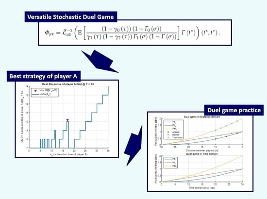
The functional ${\Phi }_{\mu \nu }$ of the game on trace σ-algebra $\mathcal{F}\left(\Omega \right)\cap \left\{P_a\left(S_{\mu }\right)+P_b\left(T_{\nu }\right)\ge 1\right\}\cap \left\{S_{\mu }\le T_{\nu }\right\}$ satisfies the following formula:

$${\Phi }_{\mu \nu }={\widehat{\mathcal{L}}}_{uv}^{-1}\left(\mathbb{E}\left[\frac{\left(1-{\gamma }_0\left(\tau \right)\right)\left(1-{\Gamma }_0\left(\sigma \right)\right)}{{\gamma }_1\left(\tau \right)\left(1-{\gamma }_2\left(\tau \right)\right){\Gamma }_1\left(\sigma \right)\left(1-\Gamma \left(\sigma \right)\right)}\right]\Gamma \left(t^{*}\right)\right)\left(t^{*},t^{*}\right).$$

(12)

Proof. 

The theorem is abbreviated as (13)–(20):

$$\begin{array}{c}\hfill \gamma \left(x,t\right)=e^{-xt},\end{array}$$

(13)

$$\begin{array}{c}\hfill {\gamma }_0\left(t\right):=\gamma \left(v,t\right),\end{array}$$

(14)

$$\begin{array}{c}\hfill {\gamma }_1\left(t\right):=\gamma \left({\vartheta }_0+v,t\right),\end{array}$$

(15)

$$\begin{array}{c}\hfill {\gamma }_2\left(t\right):=\gamma \left({\vartheta }_0+{\vartheta }_1+v,t\right)\end{array}$$

(16)

$$\begin{array}{c}\hfill {\Gamma }_0\left(t\right):=\gamma \left(u,t\right),\end{array}$$

(17)

$$\begin{array}{c}\hfill {\Gamma }_1\left(t\right):=\gamma \left({\theta }_0+u,t\right),\end{array}$$

(18)

$$\begin{array}{c}\hfill {\Gamma }_2\left(t\right):=\gamma \left({\theta }_0+{\theta }_1+u,t\right),\end{array}$$

(19)

$$\begin{array}{c}\hfill \Gamma \left(t\right):={\gamma }_2\left(t\right)·{\Gamma }_2\left(t\right).\end{array}$$

(20)

The Laplace–Carson transform is applied as follows:

$${\widehat{\mathcal{L}}}_{pq}\left(•\right)\left(u,v\right)=uv{\int }_{p=0}^{\infty }{\int }_{q=0}^{\infty }{e}^{-up-vq}\left(•\right)d\left(p,q\right),\mathrm{Re}\left(u\right)>0,\mathrm{Re}\left(v\right)>0,$$

(21)

with the inverse:

$${\widehat{\mathcal{L}}}_{uv}^{-1}\left(•\right)\left(p,q\right)={\mathcal{L}}^{-1}\left(•\frac{1}{uv}\right),$$

(22)

where ${\mathcal{L}}^{-1}$ is the inverse of the bivariate Laplace transform [23]. Let us introduce the families:

$$\begin{array}{c}\hfill \mu \left(p\right)=inf\left\{m:S_m>p\right\}\end{array}$$

(23)

$$\begin{array}{c}\hfill \nu \left(q\right)=inf\left\{n:T_n>q\right\}.\end{array}$$

(24)

Application of ${\widehat{\mathcal{L}}}_{pq}$ to ${\Phi }_{\mu \left(p\right)\nu \left(q\right)}$ will bypass all terms except for $\left\{S_{\mu }<T_{\nu }\right\}\cap \left\{P_a\left(S_{\mu }\right)+P_b\left(T_{\nu }\right)\ge 1\right\}$. Thus, applying operator ${\widehat{\mathcal{L}}}_{pq}$ to random set $\left\{{\mathbf{1}}_{\left\{\mu \left(p\right)=j,\nu \left(q\right)=k\right\}}:p\ge 0,q\ge 0\right\}$, we arrive at:

$${\widehat{\mathcal{L}}}_{pq}\left({\mathbf{1}}_{\left\{\mu \left(p\right)=j,\nu \left(q\right)=k\right\}}\right)\left(u,v\right)=\left(e^{-u{S}_{j-1}}-e^{-u{S}_j}\right)\left(e^{-v{T}_{k-1}}-e^{-v{T}_k}\right).$$

(25)

To prove the formula (25), we first notice that:

$${\mathbf{1}}_{\left\{\mu \left(p\right)=j,\nu \left(q\right)=k\right\}}=\left({\mathbf{1}}_{\left\{S_{j-1}\le p\right\}}{\mathbf{1}}_{\left\{S_j>p\right\}}\right)\left({\mathbf{1}}_{\left\{T_{k-1}\le q\right\}}{\mathbf{1}}_{\left\{T_k>q\right\}}\right).$$

(26)

Then, iterating the integral of (21), we have from (25):

$${\widehat{\mathcal{L}}}_{pq}\left({\mathbf{1}}_{\left\{\mu \left(p\right)=j,\nu \left(q\right)=k\right\}}\right)\left(u,v\right)={\int }_{p=S_{j-1}}^{S_j}{e}^{-up}dp{\int }_{q=T_{k-1}}^{T_k}{e}^{-vq}dq$$

(27)

which yields (25). Denote:

$$\Psi \left(u,v\right):={\widehat{\mathcal{L}}}_{pq}\left({\Phi }_{\mu \left(p\right)\nu \left(q\right)}\right)\left(u,v\right)$$

(28)

Since,

$$\begin{array}{c}\hfill {\Phi }_{\mu \left(p\right)\nu \left(q\right)}=\sum _{j\ge 0}\mathbb{E}\left[\sum _{k\ge 0}\mathbb{E}[e^{-{\theta }_0{S}_{j-1}-{\theta }_1{S}_j}·e^{-{\vartheta }_0{T}_{k-1}-{\vartheta }_1{T}_k}\times {\mathbf{1}}_{\left\{\mu \left(p\right)=j,\nu \left(q\right)=k\right\}}·{\mathbf{1}}_{\left\{S_{\mu }\ge t^{*},T_{\nu }>S_{\mu }\right\}}\right]\end{array}$$

(29)

where:

$${\mathbf{1}}_{\left\{S_{\mu }<T_{\nu }\right\}}·{\mathbf{1}}_{\left\{P_a\left(S_{\mu }\right)+P_b\left(T_{\nu }\right)\ge 1\right\}}={\mathbf{1}}_{\left\{S_{\mu }\ge t^{*},T_{\nu }>S_{\mu }\right\}},$$

(30)

then by Fubini’s theorem and due to (25) and (28),

$$\begin{array}{cc}\hfill \Psi \left(u,v\right)=& \sum _{j\ge 0}\mathbb{E}\left[\sum _{k>\left(t^{*}/\tau \right)}\mathbb{E}[e^{-{\theta }_0{S}_{j-1}-{\theta }_1{S}_j}·e^{-{\vartheta }_0{T}_{k-1}-{\vartheta }_1{T}_k}\left(e^{-u{S}_{j-1}}-e^{-u{S}_j}\right)\left(e^{-v{T}_{k-1}}-e^{-v{T}_k}\right)\times {\mathbf{1}}_{\left\{S_k\ge t^{*}\right\}}\right]\hfill \\ \hfill =& \mathbb{E}\left[\sum _{j\ge 0}{R}_{1j}\left[\sum _{k>\left(\frac{\sigma }{\tau }\right)j}{R}_{2jk}\right]\right]\hfill \end{array}$$

(31)

where:

$$\begin{array}{rr}\hfill R_{1j}& =e^{-\left({\theta }_0+u\right)\left(j-1\right)\sigma -{\theta }_1\sigma j}\left(1-e^{-u\sigma }\right)\times {\mathbf{1}}_{\left\{P_a\left(S_j\right)+P_b\left(T_k\right)\ge 1\right\}}\hfill \\ & =e^{\left({\theta }_0+u\right)\sigma }\left(1-e^{-u\sigma }\right){\left[e^{-\left({\theta }_0+{\theta }_1+u\right)\sigma }\right]}^j\times {\mathbf{1}}_{\left\{S_j\ge t^{*}\right\}}\hfill \\ & =e^{\left({\theta }_0+u\right)\sigma }\left(1-{\Gamma }_0\left(\sigma \right)\right){\Gamma }_2{\left(\sigma \right)}^j\times {\mathbf{1}}_{\left\{S_j\ge t^{*}\right\}},\hfill \\ \hfill R_{2k}& =e^{-\left({\vartheta }_0+v\right)\tau \left(k-1\right)-{\vartheta }_1\tau k}\left(1-e^{-v\tau }\right),\hfill \end{array}$$

and:

$$\begin{array}{rr}\hfill {\sum }_{k>\left(\frac{\sigma }{\tau }\right)j}& R_{2jk}={\sum }_{k>\left(\frac{\sigma }{\tau }\right)j}{e}^{\left({\vartheta }_0+v\right)\tau }\left(1-e^{-v\tau }\right){\left[e^{-\left({\vartheta }_0+{\vartheta }_1+v\right)\tau }\right]}^k\hfill \\ \hfill & =e^{\left({\vartheta }_0+v\right)\tau }\left(1-e^{-v\tau }\right)·\left({\sum }_{k>\left(\frac{\sigma }{\tau }\right)j}{\left[e^{-\left({\vartheta }_0+{\vartheta }_1+v\right)\tau }\right]}^k\right)\hfill \\ \hfill & =\frac{\left(1-{\gamma }_0\left(\tau \right)\right)}{{\gamma }_1\left(\tau \right)}·\frac{{\gamma }_2{\left(\sigma \right)}^j}{1-{\gamma }_2\left(\tau \right)}\hfill \end{array}$$

Then, we have:

$$\begin{array}{cc}\hfill \Psi \left(u,v\right)=& \mathbb{E}\left[\frac{\left(1-{\gamma }_0\left(\tau \right)\right)\left(1-{\Gamma }_0\left(\sigma \right)\right)}{{\gamma }_1\left(\tau \right)\left(1-{\gamma }_2\left(\tau \right)\right){\Gamma }_1\left(\sigma \right)}\left({\sum }_{j\ge \left(\frac{t^{*}}{\sigma }\right)}{\left[\Gamma \left(\sigma \right)\right]}^j\right)\right]\hfill \\ \hfill & =\mathbb{E}\left[\frac{\left(1-{\gamma }_0\left(\tau \right)\right)\left(1-{\Gamma }_0\left(\sigma \right)\right)}{{\gamma }_1\left(\tau \right)\left(1-{\gamma }_2\left(\tau \right)\right){\Gamma }_1\left(\sigma \right)}·\left(\frac{\Gamma \left(t^{*}\right)}{\left(1-\Gamma \left(\sigma \right)\right)}\right)\right].\hfill \end{array}$$

Now, ${\Phi }_{\mu \left(p\right)\nu \left(q\right)}$ can be revived when the inverse of the operator ${\widehat{\mathcal{L}}}_{pq}$ of (22) to $\Psi \left(u,v\right)$:

$${\Phi }_{\mu \nu }={\widehat{\mathcal{L}}}_{uv}^{-1}\left(\mathbb{E}\left[\frac{\left(1-{\gamma }_0\left(\tau \right)\right)\left(1-{\Gamma }_0\left(\sigma \right)\right)}{{\gamma }_1\left(\tau \right)\left(1-{\gamma }_2\left(\tau \right)\right){\Gamma }_1\left(\sigma \right)\left(1-\Gamma \left(\sigma \right)\right)}\right]\Gamma \left(t^{*}\right)\right)\left(t^{*},t^{*}\right).$$

(32)

☐

The functional ${\Phi }_{\mu \nu }$ contains all decision making parameters regarding this standard stopping game. The information includes the best moments of shooting ($S_{\mu },T_{\nu };$ exit time), the one step before the best moments ($S_{\mu -1},T_{\nu -1};$ pre-exit time), and the optimal number of iterations for both players. The information for both players from the closed functional are as follows:

For Player A:

$$\begin{array}{c}\hfill \mathbb{E}\left[S_{\mu }\right]=\underset{\theta \to 0}{lim}\left(-\frac{\partial }{\partial \theta }\right){\Phi }_{\mu \nu }\left(0,\theta ,0,0\right),\end{array}$$

(33)

$$\begin{array}{c}\hfill \mathbb{E}\left[S_{\mu -1}\right]=\underset{\theta \to 0}{lim}\left(-\frac{\partial }{\partial \theta }\right){\Phi }_{\mu \nu }\left(\theta ,0,0,0\right),\end{array}$$

(34)

For Player B:

$$\begin{array}{c}\hfill \mathbb{E}\left[T_{\nu }\right]=\underset{\vartheta \to 0}{lim}\left(-\frac{\partial }{\partial \theta }\right){\Phi }_{\mu \nu }\left(0,0,0,\vartheta \right),\end{array}$$

(35)

$$\begin{array}{c}\hfill \mathbb{E}\left[T_{\nu -1}\right]=\underset{\vartheta \to 0}{lim}\left(-\frac{\partial }{\partial \theta }\right){\Phi }_{\mu \nu }\left(0,0,\vartheta ,0\right),\end{array}$$

(36)

and:

$$\begin{array}{c}\hfill \mathbb{E}\left[\mu \right]\simeq ⌊\mathbb{E}\left[\frac{S_{\mu }}{\sigma }\right]⌋,\mathbb{E}\left[\nu \right]\simeq ⌊\mathbb{E}\left[\frac{T_{\nu }}{\tau }\right]⌋.\end{array}$$

(37)

3. Special Case: Deterministic Iteration Times

This section demonstrates the practical case of a versatile stochastic duel game that considers the deterministic iteration time of each player. As was mentioned before, this newly proposed duel game is flexible because it is capable of using any incremental cost functions in the continuous time domain. Let us assume that the optimal moment of a time based duel game is already known as $t^{*}$ from (1)–(4). Since we deal with the deterministic iteration process of each player, the duration of one iteration for each player is a constant value. From (7), (8) and (13), we have:

$$\mathbb{E}\left[e^{-\theta ·\sigma }\right]=e^{-d_a\theta },\mathbb{E}\left[e^{-\vartheta \tau }\right]=e^{-d_b\vartheta }.$$

(38)

where $d_a$ and $d_b$ are the fixed iteration duration times of the players ($d_a$ for Player A and $d_b$ for Player B).

Lemma 1.

The functional ${\Phi }_{\mu \nu }$ based on the fixed iteration duration (38) is as follows:

$${\Phi }_{\mu \nu }\left({\theta }_0,{\theta }_1,{\vartheta }_0,{\vartheta }_1\right)={\alpha }_0^{*}{\alpha }_1^{*}{\alpha }_1{\beta }_0^{*}{\beta }_1^{*}{\beta }_1,$$

(39)

where:

$$\begin{array}{c}\hfill {\alpha }_0^{*}=e^{-t^{*}{\theta }_0},{\alpha }_1^{*}=e^{-t^{*}{\theta }_1},{\alpha }_1=e^{-u{\theta }_1},\end{array}$$

(40)

$$\begin{array}{c}\hfill {\beta }_0^{*}=e^{-t^{*}{\vartheta }_0},{\beta }_1^{*}=e^{-t^{*}{\vartheta }_1},{\beta }_0=e^{-v{\vartheta }_0}.\end{array}$$

(41)

Proof. 

From (13), let us assign (14)–(20) as follows:

$$\begin{array}{c}\hfill {\gamma }_0^b:={\gamma }_0\left(d_b\right)=e^{-d_{b}v},\end{array}$$

(42)

$$\begin{array}{c}\hfill {\gamma }_1^b:={\gamma }_1\left(d_b\right)=e^{-d_b\left({\vartheta }_0+v\right)}={\beta }_0·{\gamma }_0^b,\end{array}$$

(43)

$$\begin{array}{c}\hfill {\gamma }_2^b:={\gamma }_2\left(d_b\right)=e^{-d_b\left({\vartheta }_0+{\vartheta }_1+v\right)}={\beta }_2·{\gamma }_0^b={\beta }_0{\beta }_1·{\gamma }_0^b,\end{array}$$

(44)

$$\begin{array}{c}\hfill {\gamma }_0^a={\Gamma }_0\left(d_a\right)=e^{-d_{a}u},\end{array}$$

(45)

$$\begin{array}{c}\hfill {\gamma }_1^a={\Gamma }_1\left(d_a\right)=e^{-d_a\left({\theta }_0+u\right)}={\alpha }_0·{\gamma }_0^a,\end{array}$$

(46)

$$\begin{array}{c}\hfill {\gamma }_2^a={\Gamma }_2\left(d_a\right)=e^{-d_a\left({\theta }_0+{\theta }_1+u\right)}={\alpha }_2·{\gamma }_0^a={\alpha }_0{\alpha }_1·{\gamma }_0^a,\end{array}$$

(47)

$$\begin{array}{c}\hfill {\Gamma }_b^{*}{\Gamma }_a^{*}:=\Gamma \left(t^{*}\right)={\gamma }_2\left(t^{*}\right)·{\Gamma }_2\left(t^{*}\right)=\left({\beta }_0^{*}{\beta }_1^{*}{\gamma }_{*}^b\right)\left({\alpha }_0^{*}{\alpha }_1^{*}{\gamma }_{*}^a\right)\end{array}$$

(48)

Recalling Theorem 1 from (32), we have:

$$\begin{array}{cc}\hfill {\Phi }_{\mu \nu }=& {\widehat{\mathcal{L}}}_{uv}^{-1}\left(\mathbb{E}\left[\frac{\left(1-{\gamma }_0\left(\tau \right)\right)}{{\gamma }_1\left(\tau \right)\left(1-{\gamma }_2\left(\tau \right)\right)}\right]\mathbb{E}\left[\frac{\left(1-{\Gamma }_0\left(\sigma \right)\right)\Gamma \left(t^{*}\right)}{{\Gamma }_1\left(\sigma \right)\left(1-\Gamma \left(\sigma \right)\right)}\right]\right)\left(t^{*},t^{*}\right)\hfill \\ \hfill & =\left\{{\widehat{\mathcal{L}}}_v^{-1}\left(\mathbb{E}\left[\frac{\left(1-{\gamma }_0\left(\tau \right)\right)}{{\gamma }_1\left(\tau \right)\left(1-{\gamma }_2\left(\tau \right)\right)}\right]\right)\left(t^{*}\right)\right\}\left\{{\widehat{\mathcal{L}}}_u^{-1}\left(\mathbb{E}\left[\frac{\left(1-{\Gamma }_0\left(\sigma \right)\right)\Gamma \left(t^{*}\right)}{{\Gamma }_1\left(\sigma \right)\left(1-\Gamma \left(\sigma \right)\right)}\right]\right)\left(t^{*}\right)\right\}\hfill \\ \hfill & ={\widehat{\mathcal{L}}}_v^{-1}\left\{L_2\right\}\left\{L_1\right\},\hfill \end{array}$$

(49)

where:

$$\begin{array}{cc}\hfill \left\{L_1\right\}=& {\widehat{\mathcal{L}}}_u^{-1}\frac{\left(1-{\gamma }_0^a\right){\Gamma }_a^{*}}{{\gamma }_1^a\left(1-{\gamma }_2^a{\gamma }_2^b\right)}={\widehat{\mathcal{L}}}_u^{-1}\frac{{\Gamma }_a^{*}}{{\gamma }_1^a\left(1-{\gamma }_2^a{\gamma }_2^b\right)}-{\widehat{\mathcal{L}}}_u^{-1}\frac{{\gamma }_0^a{\Gamma }_a^{*}}{{\gamma }_1^a\left(1-{\gamma }_2^a{\gamma }_2^b\right)}\hfill \\ \hfill & =\left({\alpha }_2^{*}{\alpha }_1\right)\left({\beta }_0{\beta }_1\right)e^{-d_{b}v},\hfill \end{array}$$

(50)

$$\begin{array}{c}{\widehat{\mathcal{L}}}_u^{-1}\left\{\frac{{\Gamma }_a^{*}}{{\gamma }_1^a\left(1-{\gamma }_2^a{\gamma }_2^b\right)}\right\}\left(t^{*}\right)=\left(\frac{{\alpha }_2^{*}}{{\alpha }_0}\right)\left(1+\left({\alpha }_2{\beta }_2\right)e^{-d_{b}v}\right),\hfill \end{array}$$

$$\begin{array}{c}{\widehat{\mathcal{L}}}_u^{-1}\left\{\frac{{\gamma }_0^a{\Gamma }_a^{*}}{{\gamma }_1^a\left(1-{\gamma }_2^a{\gamma }_2^b\right)}\right\}\left(t^{*}\right)=\left(\frac{{\alpha }_2^{*}}{{\alpha }_0}\right).\hfill \end{array}$$

From (49),

$$\begin{array}{cc}\hfill \left\{L_2\right\}=& \mathbb{E}\left[\frac{\left(1-{\gamma }_0\left(\tau \right)\right)}{{\gamma }_1\left(\tau \right)\left(1-{\gamma }_2\left(\tau \right)\right)}\right]\hfill \\ \hfill & =\left\{\frac{{\Gamma }_b^{*}}{{\gamma }_1^b\left(1-{\gamma }_2^b\right)}\right\}-\left\{\frac{{\gamma }_0^b{\Gamma }_b^{*}}{{\gamma }_1^b\left(1-{\gamma }_2^b\right)}\right\}=L_{21}-L_{22},\hfill \end{array}$$

(51)

where:

$$\begin{array}{c}\hfill L_{21}=\frac{{\beta }_2^{*}}{{\beta }_0}\sum _{j\ge 0}{\left({\beta }_2\right)}^j{e}^{-\left\{\left(j-1\right)d_b+t^{*}\right\}v},\end{array}$$

(52)

$$\begin{array}{c}\hfill L_{22}=\frac{{\beta }_2^{*}}{{\beta }_0}\sum _{j\ge 0}{\left({\beta }_2\right)}^j{e}^{-\left\{j·d_b+t^{*}\right\}v}.\end{array}$$

(53)

From (50)–(53),

$$\begin{array}{c}{\Phi }_{\mu \nu }={\widehat{\mathcal{L}}}_v^{-1}\left\{L_{21}\right\}\left\{\left({\alpha }_2^{*}{\alpha }_1\right)\left({\beta }_0{\beta }_1\right)e^{-d_{b}v}\right\}-{\widehat{\mathcal{L}}}_v^{-1}\left\{L_{22}\right\}\left\{\left({\alpha }_2^{*}{\alpha }_1\right)\left({\beta }_0{\beta }_1\right)e^{-d_{b}v}\right\}=R_1-R_2,\hfill \end{array}$$

where:

$$\begin{array}{cc}\hfill R_1& =\left({\alpha }_2^{*}{\alpha }_1\right)\left({\beta }_0{\beta }_1\right){\widehat{\mathcal{L}}}_v^{-1}\left\{{\sum }_{j\ge 0}{\left({\beta }_2\right)}^j{e}^{-\left\{\left(j-1\right)d_b+t^{*}\right\}v}\right\}\left\{e^{-d_{b}v}\right\}\hfill \\ \hfill & =\left({\alpha }_2^{*}{\alpha }_1\right)\left({\beta }_0{\beta }_1\right)\left(\frac{{\beta }_2^{*}}{{\beta }_0}\right){\sum }_{j\ge 0}{\left({\beta }_2\right)}^j{\mathbf{1}}_{\left\{j\le 0\right\}}=\left({\alpha }_2^{*}{\alpha }_1\right)\left({\beta }_0{\beta }_1\right)\left(\frac{{\beta }_2^{*}}{{\beta }_0}\right),\hfill \end{array}$$

$$\begin{array}{cc}\hfill R_2& =\left({\alpha }_2^{*}{\alpha }_1\right)\left({\beta }_0{\beta }_1\right){\widehat{\mathcal{L}}}_v^{-1}\left\{{\sum }_{j\ge 0}{\left({\beta }_2\right)}^j{e}^{-\left\{j{d}_b+t^{*}\right\}v}\right\}\left\{e^{-d_{b}v}\right\}\hfill \\ \hfill & =\left({\alpha }_2^{*}{\alpha }_1\right)\left({\beta }_0{\beta }_1\right)\left(\frac{{\beta }_2^{*}}{{\beta }_0}\right){\sum }_{j\ge 0}{\left({\beta }_2\right)}^j{\mathbf{1}}_{\left\{j\le -1\right\}}=0.\hfill \end{array}$$

Therefore, we have:

$${\Phi }_{\mu \nu }=\left({\alpha }_2^{*}{\alpha }_1\right)\left({\beta }_0{\beta }_1\right)\left(\frac{{\beta }_2^{*}}{{\beta }_0}\right)={\alpha }_0^{*}{\alpha }_1^{*}{\alpha }_1{\beta }_0^{*}{\beta }_1^{*}{\beta }_1.$$

(54)

☐

From (33) and (35), the information for both players to get the optimal moment of shooting is as follows:

$$\mathbb{E}\left[S_{\mu }\right]=t^{*}+d_a,\mathbb{E}\left[T_{\nu }\right]=t^{*}+d_b,$$

(55)

$$\mathbb{E}\left[\mu \right]\simeq ⌊\frac{t^{*}+d_a}{d_a}⌋,\mathbb{E}\left[\nu \right]\simeq ⌊\frac{t^{*}+d_b}{d_b}⌋.$$

(56)

The actual moment of the best shot may not be the same as (33) and (36) because the exit index of each player should be an integer, and this fact also impacts the pre-exit time of each player:

$$\mathbb{E}\left[S_{\mu -1}\right]=d_a⌊\frac{t^{*}}{d_a}⌋,\mathbb{E}\left[T_{\nu -1}\right]=d_b⌊\frac{t^{*}}{d_b}⌋.$$

(57)

3.1. Best Strategies for Player A

The best response is the strategies that produce the most favorable outcomes for a player [24]. The best response of Player A is the exit index of shooting $\mu$, and he/she responds based on the iteration time of Player B. Let us assign the function of the best response correspondences for Player A as follows:

$$\mu \left(d_b\right)=\left(⌊\left(\frac{d_b}{d_a}\right)\left(⌊\frac{t^{*}+d_b}{d_b}⌋\right)⌋\right).$$

(58)

As a demonstration, we take $t^{*}=35,$$d_a=5$ and $d_b\in \left[0.01,t^{*}\right]$, and each iteration process of each player is deterministic. The analysis for the best response of Player A is illustrated in Figure 1.

From (56) and (58), the best response index depends on the iteration duration of Player B when the iteration period of Player A is five. For instant, the exit index of Player A is 10 when the iteration period of Player B is 17 (i.e., $d_b=17$). This means that Player A should take the shot at the 17th iteration to get the highest chance to hit Player B. From (56), the exit time of Player A gives the best hitting chance, and the hitting probability of Player A is $P_a\left(10d_a\right)$ from (1) and (3).

3.2. Reconstructing a Conventional Duel Game

The distance based conventional duel game [4] is a special case of the versatile stochastic duel game under the deterministic iteration time condition. This section demonstrates how the duel game in the time domain could be adapted to analyze a conventional duel game. As was mentioned in the previous section, a conventional duel game was adapted from Polak [4]. Let us consider the duel game, which has the following rules:

• Each player (Players A, B) has a gun with a single bullet, and Player A starts the game;
• they are facing each other with a distance of L$\left(=30\left[\mathrm{m}\right]\right)$;
• let $P_a\left(l\right)$ be the probability of Player A hitting Player B if Player A shoots at distance l;
• let $P_b\left(l\right)$ be Player B’s probability of hitting Player A if Player B shoots at distance l;
• the probability of hitting for each player is give as follows:

  $$P_a\left(l\right)=\frac{1}{L^2}{\left(L-l\right)}^2,P_b\left(l\right)=1-\frac{1}{L}·l,0\le l\le L,$$

  (59)
• players alternatively have the chance to make the decision;
• either “shoot” or “one step $\left(l_0=2\left[\mathrm{m}\right]\right)$ forward”;
• every turn makes $2l_0$$\left(=4\left[\mathrm{m}\right]\right)$ closer to each other if both players are moving forward instead of shooting;
• the hitting probabilities of both players are known (i.e., perfect information).

According to the above rules, the illustration of the hitting probabilities of both players is shown in Figure 2.

The first shot should occur after $l^{*}$, and no one should do so before $l^{*}$. Player A knows the next move of Player B [7] based on the given game rules, and whoever gets the first turn after $l^{*}$ will be the winner of the game. The value $l^{*}$ is determined by their joint probabilities from (4):

$$l^{*}=\inf \left\{0\le l\le L:P_a\left(l\right)+P_b\left(l\right)\ge 1\right\}.$$

(60)

According to the above given conditions, $l^{*}$ yields $11.459\left[\mathrm{m}\right]$, and Player A has a greater chance of winning this game when Player A shoots at his/her fifth turn. Again, it is noted that who shoots first is not necessarily a better or a worse shooter [4]. This typical duel problem could be solvable by transforming the distance domain to the time domain. Let us assume the speed for “moving-forward” v is 1 $\left[\mathrm{m}/\mathrm{s}\right]$, which is constant. All variables in the distance domain are easily transformed to the time domain (see

Table 1. Time domain transform of a classic duel game.

Distance Domain	Deterministic Time Domain
$L=30$$\left[\mathrm{m}\right]$	$t_{\max }=\frac{L}{v}=30$$\left[\sec \right]$
l	$t=t_{\max }-\frac{l}{v}$
$l^{*}=11.459$$\left[\mathrm{m}\right]$	$t^{*}=18.541$$\left[\sec \right]$
$2l_0=4$$\left[\mathrm{m}\right]$	$d_a=d_b=4$$\left[\sec \right]$
$P_a\left(l\right)=\frac{1}{{30}^2}{\left(30-l\right)}^2$	$P_a\left(t\right)=\frac{1}{{\left(1·30\right)}^2}·t^2$
$P_b\left(l\right)=1-\frac{1}{30}·l$	$P_b\left(t\right)=\frac{1}{30}·t$

).

The hitting probabilities in the distance and the time domains are illustrated in Figure 3. It provides the mapping of hitting probabilities between two domains.

As is illustrated in Figure 3, the hitting probabilities in both domains are the same, but the input variable has been changed to time (seconds) from distance (meters). Once the distance domain is mapped in the time domain, we can find the best response $\mu \left(\nu \left(d_a\right)\right)$ from (59), which is graphically demonstrated in Figure 4.

The best response function of Player A shows all iteration time ranges of Player B, and the best strategy of Player A in this duel game is shooting at the fifth iteration moment where $d_b=d_a$ (i.e., the downward-pointing triangle in Figure 4).

4. Case: New Product Launching Strategy

This section demonstrates a practical application for developing a marketing strategy, and this case shows how to apply the proposed versatile stochastic duel game. The numbers and names were fictional, but realistic for this demonstration. Two major smartphone companies were considered, and let us create some stories as follows: Samsung just finished developing the flagship smartphone for this year. Samsung should decide to either “launch” the smartphone or “wait” to develop new additional features. One development cycle takes approximately six months. Once a development cycle is started, they cannot launch the product until it is completed. In other words, Samsung must wait six months for their next opportunity to make another decision once they decide to “wait.” Samsung knows that Apple completes the flagship smartphone five months later, and it takes four months to add new additional features by Apple after completing the initial product. Since both companies have ample experience in the smartphone industry, they know the probability of success for either choice. Samsung wants to know the best time to launch their new flagship smartphone. If the flagship product is launched too early, consumers would not choose the product because it would not have enough new technologies to be attractive. However, Samsung may also lose the game if Apple launches their flagship device before Samsung launches. This versatile duel game could be easily demonstrated to provide the best strategies for Samsung (and Apple). It is noted that this section is designed only for showing how the mathematical model could be applied in the marketing decision problem. Hence, this section only provides the condensed results. The development cycles of both companies are assumed to be exponentially distributed, and the parameters based on the current scenario are shown in

Table 2. Initial setup values for the case study.

Parameter	Value	Description
$\widetilde{{\delta }_0}\left(=\mathbb{E}\left[S_0\right]\right)$	0	Initial development cycle of Samsung
$\tilde{\delta }\left(=\mathbb{E}\left[\sigma \right]\right)$	6	Development cycle of Samsung
$\mathbb{E}\left[T_0\right]$	5	Initial development cycle of Apple (after Samsung)
$\mathbb{E}\left[\tau \right]$	4	Development cycle of Apple

.

It is noted that some parameters of this setup, including the development cycles, were not carefully evaluated, but were realistic because these were chosen based on information from experts in the smartphone industry. Once all the parameters were mapped, we could get the decision parameters from the simulated results in

Table 3. Simulated results of the case.

Parameter	Value	Description
$t^{*}$	$17.95$	Best moment that whichever player wins the game
$\mathbb{E}\left[\mu \right]$	3	Number of development cycles that is best for Samsung
$\mathbb{E}\left[S_{\mu }\right]$	18	Best time to launch the product for Samsung
$\mathbb{E}\left[\nu \right]$	4	Number of development cycles that is best for Apple
$\mathbb{E}\left[T_{\nu }\right]$	21	Best time to launch the product for Apple

.

According to the simulated results, Samsung had the opportunity to launch the flagship product after passing the moment $t^{*}$, but before Apple launched the product. However, Samsung should run at least three development cycles to add new features before launching (i.e., $\mu =3$) after the first commercially ready product was developed $\left(=S_0\right)$. If both companies launched their flagship smartphones before 18 months $\left(<t^{*}\right)$, customers would not buy their products because they lacked attractive features. In the setup of the above scenario, Samsung was mostly likely to win the game because the best moment of shooting by Samsung $\left(=S_{\mu }\right)$ was closer to the threshold $t^{*}$ than what Apple had (i.e., $t^{*}<S_{\mu }<T_{\nu }$). In this particular scenario, releasing the smartphone on $T_{\nu }$ by Apple was no longer the optimal strategy. Therefore, it might be better for Apple to take the risk to launch the product at $T_{\nu -1}$ ($=17$ months) instead of $T_{\nu }$ ($=21$ months) because Apple would lose this game when Samsung launched the flagship product at $S_{\mu }$. Apple would stochastically lose this game, but it is noted that the solution of the game was not deterministic. In other words, a player with a higher probability of success was not guaranteed to win a game.

5. Conclusions

A new type of antagonistic stochastic duel game was studied. In this versatile stochastic duel game, both players could have random iterations in the time domain. A joint functional of the standard stopping game was constructed to analyze the decision making parameters, which indicated the best winning strategies of players in the time domain stochastic game. Compact closed forms from the Laplace–Carson transforms were obtained, and the hybrid stochastic game model was more flexible to solve various duel-type game problems more effectively. The analytical approach by applying the proposed model to a conventional duel game was fully described for better understanding the core of the model. Furthermore, an actual application in the smartphone market was provided for the direct implementation of a versatile stochastic duel game in real-world decision making situations. An extended version of the duel-type game for multiple players is currently under development as a successor of this research.

References

- Kim, S.-K.; Yeun, C.Y.; Damiani, E.; Al-Hammadi, Y.; Lo, N.-W. New Blockchain Adoptation For Automotive Security by Using Systematic Innovation. In Proceedings of the 2019 IEEE Transportation Electrification Conference and Expo Asia-Pacific, Jeju, Korea, 8–10 May 2019; pp. 1–4. [Google Scholar]
- Kim, S.-K. Blockchain Governance Game. Comp. Indust. Eng. 2019, 136, 373–380. [Google Scholar] [CrossRef] [Green Version]
- Moschini, G. Nash equilibrium in strictly competitive games: Live play in soccer. Econ. Lett. 2004, 85, 365–371. [Google Scholar] [CrossRef]
- Polak, B. Discussion of Duel. Open Yale Courses. 2008. Available online: http://oyc.yale.edu/economics/econ-159/lecture-16 (accessed on 1 May 2019).
- Dshalalow, J.H.; Iwezulu, K. Discrete versus continuous operational calculus in antagonistic stochastic games. Sao Paulo J. Math. Sci. 2017, 11, 471–489. [Google Scholar] [CrossRef]
- Dshalalow, J.H. Random Walk Analysis in Antagonistic Stochastic Games. Stoch. Anal. Appl. 2008, 26, 738–783. [Google Scholar] [CrossRef]
- Dshalalow, J.H.; Iwezulu, K.; White, R.T. Discrete Operational Calculus in Delayed Stochastic Games. 2019. Available online: https://arxiv.org/abs/1901.07178 (accessed on 1 May 2019).
- Kingston, C.G.; Wright, R.E. The deadliest of games: The institution of dueling. South. Econ. J. 2010, 76, 1094–1106. [Google Scholar] [CrossRef] [Green Version]
- Konstantinov, R.V.; Polovinkin, E.S. Mathematical simulation of a dynamic game in the enterprise competition problem. Cybern. Syst. Anal. 2004, 40, 720–725. [Google Scholar] [CrossRef]
- Dshalalow, J.H.; Huang, W.; Ke, H.-J.; Treerattrakoon, A. On Antagonistic Game With a Constant Initial Condition. Marginal Functionals and Probability Distributions. Nonlinear Dyn. Syst. Theory 2016, 16, 268–275. [Google Scholar]
- Azzone, G.; Pozza, I.D. An integrated strategy for launching a new product in the biotech industry. Manag. Decis. 2003, 41, 832–843. [Google Scholar] [CrossRef]
- Kam, S.; Wong, S.; Tong, C. The influence of market orientation on new product success. Eur. J. Innov. Manag. 2012, 15, 99–121. [Google Scholar]
- Kalish, S.; Mahajan, V.; Muller, E. Waterfall and sprinkler new-product strategies in competitive global markets. Int. J. Res. Mark. 1995, 12, 105–119. [Google Scholar] [CrossRef]
- Krider, R.E.; Weinberg, C.B. Competitive Dynamics and the Introduction of New Products: The Motion Picture Timing Game. J. Mark. Res. 1998, 35, 1–15. [Google Scholar] [CrossRef]
- Radas, S.; Shugan, S.M. Seasonal Marketing and Timing New Product Introductions. J. Mark. Res. 1998, 35, 296–315. [Google Scholar] [CrossRef] [Green Version]
- Tholke, J.M.; Hultinka, E.J.; Robbenb, H.S.J. Launching new product features: A multiple case examination. J. Prod. Innov. Manag. 2001, 18, 3–14. [Google Scholar] [CrossRef]
- Wind, Y.; Robertson, T.S. Marketing Strategy: New Directions for Theory and Research. J. Mark. 1983, 42, 12–25. [Google Scholar] [CrossRef]
- Lang, J.P.; Kimeldorf, G. Duels with continuous firing. Manag. Sci. 1975, 22, 470–476. [Google Scholar] [CrossRef]
- Lang, J.P.; Kimeldorf, G. Silent Duels with Nondiscrete Firing. SIAM J. Appl. Math. 1976, 31, 99–110. [Google Scholar] [CrossRef]
- Radzik, T. Games of Timing Related to Distribution of Resources. J. Optmization Theory Appl. 1988, 58, 443–471. [Google Scholar] [CrossRef]
- Radizik, T. Silent Mixed Duels. Optimization 1989, 20, 553–556. [Google Scholar] [CrossRef]
- Schwalbe, U.; Walker, P. Zermelo and the Early History of Game Theory. Games Econ. Behav. 2001, 34, 123–137. [Google Scholar] [CrossRef] [Green Version]
- Dshalalow, J.H. First excess level process. In Advances in Queueing; CRC Press: Boca Raton, FL, USA, 1995; pp. 244–261. [Google Scholar]
- Dshalalow, J.H.; Ke, H.-J. Layers of noncooperative games. Nonlinear Anal. 2009, 71, 283–291. [Google Scholar] [CrossRef]
- Kim, S.-K.; Dshalalow, J.H. Stochastic disaster rcovery systems with external resources. Math. Comput. Model. 2002, 36, 1235–1257. [Google Scholar] [CrossRef]
Figure 1.
Best response function of Player A.
Figure 2.
Probability of hitting for both players.
Figure 3.
Probability of hitting in the distance and the time domain.
Figure 4.
Best response function of Player A in the conventional duel game.