Improving the Accuracy of Convolutional Neural Networks by Identifying and Removing Outlier Images in Datasets Using t-SNE

Abstract

In the field of supervised machine learning, the quality of a classifier model is directly correlated with the quality of the data that is used to train the model. The presence of unwanted outliers in the data could significantly reduce the accuracy of a model or, even worse, result in a biased model leading to an inaccurate classification. Identifying the presence of outliers and eliminating them is, therefore, crucial for building good quality training datasets. Pre-processing procedures for dealing with missing and outlier data, commonly known as feature engineering, are standard practice in machine learning problems. They help to make better assumptions about the data and also prepare datasets in a way that best expose the underlying problem to the machine learning algorithms. In this work, we propose a multistage method for detecting and removing outliers in high-dimensional data. Our proposed method is based on utilising a technique called t-distributed stochastic neighbour embedding (t-SNE) to reduce high-dimensional map of features into a lower, two-dimensional, probability density distribution and then use a simple descriptive statistical method called interquartile range (IQR) to identifying any outlier values from the density distribution of the features. t-SNE is a machine learning algorithm and a nonlinear dimensionality reduction technique well-suited for embedding high-dimensional data for visualisation in a low-dimensional space of two or three dimensions. We applied this method on a dataset containing images for training a convolutional neural network model (ConvNet) for an image classification problem. The dataset contains four different classes of images: three classes contain defects in construction (mould, stain, and paint deterioration) and a no-defect class (normal). We used the transfer learning technique to modify a pre-trained VGG-16 model. We used this model as a feature extractor and as a benchmark to evaluate our method. We have shown that, when using this method, we can identify and remove the outlier images in the dataset. After removing the outlier images from the dataset and re-training the VGG-16 model, the results have also shown that the accuracy of the classification has significantly improved and the number of misclassified cases has also dropped. While many feature engineering techniques for handling missing and outlier data are common in predictive machine learning problems involving numerical or categorical data, there is little work on developing techniques for handling outliers in high-dimensional data which can be used to improve the quality of machine learning problems involving images such as ConvNet models for image classification and object detection problems.

1. Introduction

Machine learning (ML) has shown huge advances in recent years. The potential of this field has also been elevated across a wide range of applications including image recognition [1,2,3,4], speech recognition [5,6,7], medical diagnosis [8,9,10], defect detection and construction health assessment [11,12,13,14,15,16,17].

These recent advances in machine learning are attributed to several factors including the development of self-learning statistical models which allow computer systems to perform specific (human-like) tasks relying only on the learnt patterns, and also to the increase in computer processing power which support the analytical capabilities of these models [18,19,20]. In addition, the availability of enormous data in recent years, which allowed machine learning models to train on a large pool of examples is what gives machine learning their power [21]. Since machine learning is a “data-driven” field of artificial intelligence (AI), the quality of an ML model will be only as good or as bad as the data used to train the model [22]. The presence of outliers in the training data may lead to unreliable or even wrongly identified models [23,24]. Moreover, incorrect estimation of model parameters may also give rise to erroneous conclusions. A simple example to illustrate the effect of unwanted outliers on the results of data analysis is in statistical analysis, where the presence of outliers in the data can significantly affect the estimation of the mean and/or standard deviation of a sample data, which can lead to either over- or under-estimated values [25].

An outlier is defined as a data point that differs significantly from other data points within a given dataset [26,27,28]. Also known as abnormalities, anomalies, or deviants, outliers can occur naturally in any given distribution, for example, they may be a result of misprint errors, misplaced decimal points, transmission errors, or during exceptional circumstances such as earthquakes which can cause spikes in the measured data. The problem, as demonstrated earlier, is that only a few outliers are sometimes enough to distort the group results by altering the mean, variance, or by increasing variability of data.

Current studies have shown that data analysis is considerably dependent on how outliers or missing values are treated [24,29,30,31,32,33]. Subsequently, many methods which address this issue have been proposed including [34], which suggests adding sparsity constraints to the data as a way to remove noise. Other work such as [35] proposed a way to achieve better performance by combining sparsity constraints with spatial information.

In addition to enforcing sparsity constraints, there are other statistical methods for identifying and handling outliers: for example, such as the one presented by Kubica et al. [36], which uses an approach to identify corrupted fields, and then use the remaining non-corrupted fields to perform subsequent analysis. The authors argue that the proposed approach learns about a probabilistic model through three different components: a generative model of the clean data points, a generative model of the noise values, and a probabilistic model of the corruption process. Another method for handling outliers is based on rule creation such as the one proposed by Khoshgoftaar et al. [37]. Their approach is based on detecting noisy instances based on Boolean rules generated from the measurement data. They injected clean dataset, extracted from a NASA project for real-time predictions, with different levels of artificial noise and compared their approach to a classification filter designed to eliminate misclassified instances as noisy data. The authors demonstrated that their approach has outperformed the classification filter in detecting noisy instances at different noise levels. Clustering techniques, otherwise known as density-based, are clustering algorithms used for the task of class identification in a spatial database [38]. In their work on identifying density-based local outliers, Breunig et al. [39] assign each object a degree of being an outlier called the local outlier factor (LOF) depending on how isolated the object is concerning the surrounding neighbourhood. The authors used real-world datasets to demonstrate that such a method can be used to allocate meaningful outliers that cannot be identified using other existing approaches. Other handling methods include noise reduction which uses the 3-nearest neighbour classifier [40] and the voting ensemble [41,42] to identify and remove mislabelled occurrences.

According to Committee et al. [28], the need for outlier detection becomes particularly important when a similar type of data is gathered from $N$ different groups to ensure which groups may cause outliers [28]. The authors discuss some statistical data preparation and management techniques which address data of this nature including regression analysis techniques such as the one proposed by Gentleman et al. [33], which aims at detecting outliers by using simple residuals adjusted by the predicted values and standardised residuals against the observed values. Support vector regression methods such as the one presented by Seo et al. [43] are outlier detection methods used for nonlinear functions with multi-dimensional input. The authors argue that standard support vector regression models, although they have achieved good performance, have practical issues in computational cost and parameter adjustments. The authors propose a “practical approach” to outlier detection using support vector regression which reduces computational time and defines outlier threshold suitably.

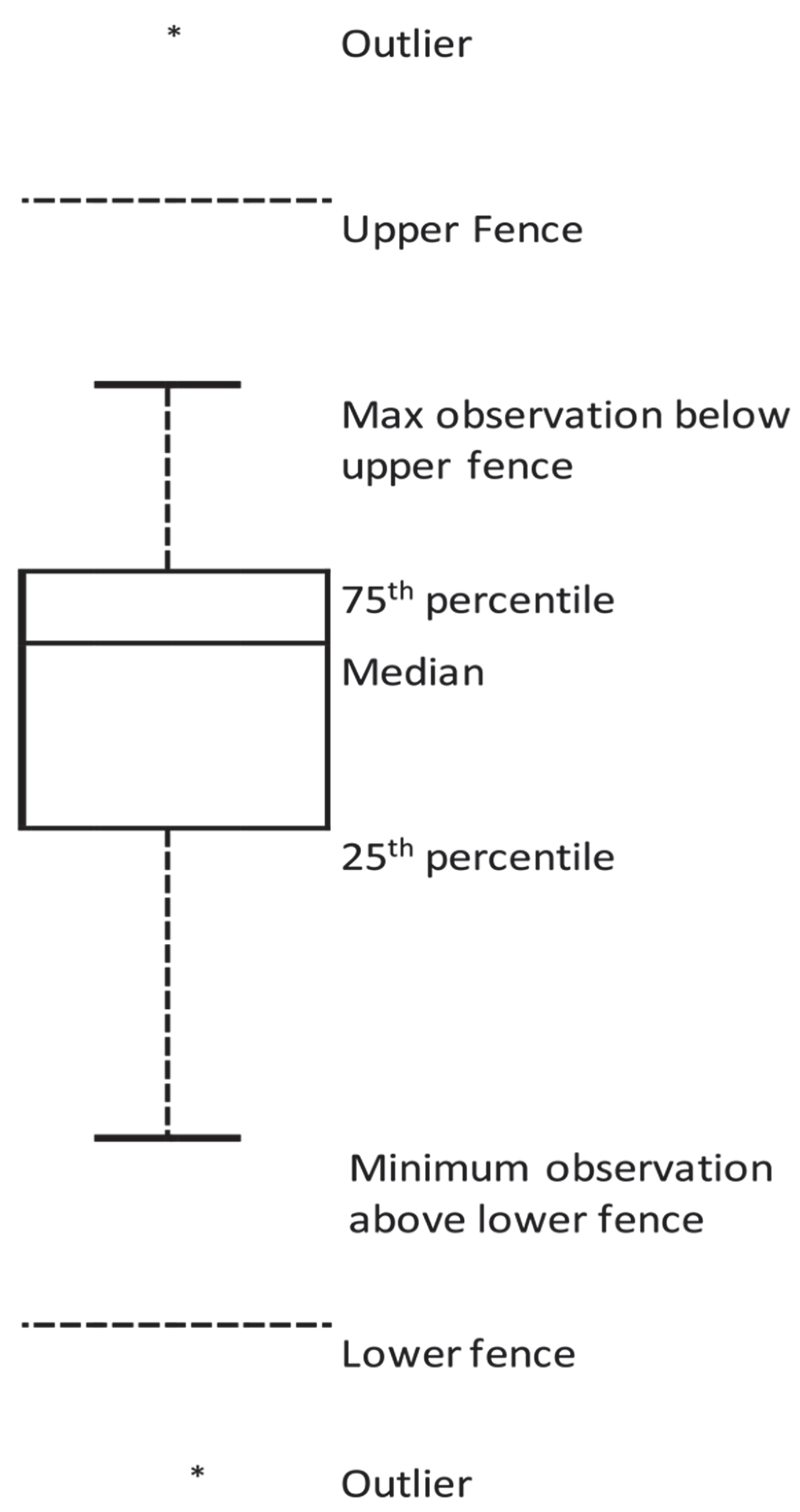
Amongst all the other methods, perhaps the simplest methods for studying outlier identification are the ones based on the mean and variance of each group of data such as the one presented by Burke et al. [32], which is also the one adopted in this study. Simple plotting methods such as the boxplot shown in Figure 1 can be particularly useful to visualise the distribution of normal and outlier data points.

In this current work, we start our research by asking the following questions: Can we determine outlier images in a class of images within training datasets? If so, can we improve the classification accuracy if the outlier images are eliminated? To answer these questions, we developed a multistage method based on using t-SNE to convert a high-dimensional vector of features extracted from images into low-dimensional probability density distribution based on similarities between these features. We then use the Interquartile range (IQR) measure, a simple descriptive statistical method, to identify any outlier values from the probability density distribution of the features. Our research is motivated by a similar work by Li et al. [44] on detecting and removing outliers from a training dataset to improve the accuracy of a machine learning model developed for multispectral burn diagnostic imaging. The authors used a dataset containing six different types of images: healthy, partial burn injury, full burn injury, blood, wound bed, and hyperaemia. The proposed method, which is based on the Z-test and univariate analysis, utilises the concepts of the maximum likelihood estimation [45] to estimate the mean and the standard deviation of a selected sub-sample located around the mean of the sample space. By firstly adjusting the size of the sub-set, and, secondly, weighing the probability distribution to generate a threshold, they were able to exclude potential outliers in the dataset. The originality of our work is in utilising t-SNE, to recursively generate a 2-dimensional probability distribution density of features extracted from each image in a dataset, and re-positioning the images depending on the degree of similarities between their features. By achieving this, all images that have features lay beyond the upper and lower fence are eliminated. Our proposed method can work with all image datasets intended for training ConvNets.

There are three main stages involved in our proposed method, feature extraction using pre-trained ConvNets, high-dimensionality-reduction using t-SNE, and, finally, determining the outliers. In the next section, we will introduce the concept of t-SNE with a mathematical representation. Next, we present a discussion about outlier handling, and, finally, transfer learning as feature extraction.

2. t-Distributed Stochastic Neighbour Embedding (t-SNE)

t-distributed stochastic neighbour embedding (or t-SNE) is a machine learning algorithm, developed by Laurens van der Maaten and Geoffrey Hinton [45] to visualise high-dimensionality data by assigning each data point a location in a two or three-dimensional map. They refer to high-dimensional data as data that require more than two or three dimensions to represent [46].

Nowadays, many machine learning applications including convolutional neural network for image classification, segmentation and labelling [47,48,49,50], and natural language processing NLP [51,52] deal with varying (low-to-high) dimensionality data. For example, in bioinformatics, a study of cancerous tumours may require tens of variables to model the changes that occur at the cellular- and tissue-level [53,54,55,56]. In signal and image processing studies, an image is represented by sets containing the colour intensity of every pixel of that image. A small image of dimensions 28 × 28 is represented by a 784-dimensional vector, and each dimension (also referred to as feature) corresponds to a one-pixel value. High-dimensional data such as images often require effective feature selection methods in order to obtain optimal accuracy [57].

t-SNE belongs to a group of non-linear dimensionality reduction techniques which also include Sammon mapping, curvilinear components analysis (CCA), Stochastic Neighbour Embedding (SNE), Locally Linear Embedding, Maximum Variance Unfolding, and Laplacian Eigenmaps [50]. There are also linear dimensionality reduction techniques which include Principal Components Analysis (PCA), and the classical multidimensional scaling (MDS) [50]. Dimensionality reduction methods, in general, aim to save as much important information about the structure of the high-dimensional data as possible during the transformation to the low-dimensional map. This is accomplished by modelling each high-dimensional object by a lower-dimensional (two- or three-dimensional) point in a way where similar objects with high probability will group by nearby points while those objects with lower probability will tend to group by distant points. This transformation (mapping) is most significant when the data (such as images) exist on multiple, but related, low-dimensional spaces including images and objects from multiple classes seen from multiple viewpoints [45]. In the context of machine learning, one can look at the transformation from high- to low-dimension (mapping) as a preliminary feature selection step after which pattern recognition algorithms are applied.

3. Mathematical Notation

Given a vector $\overline{v}$ of $N$ high-dimensional points $x_1$, $x_2$,$\cdots$ $x_n$, the Euclidean distances between a point $x_i$ and a point $x_j$ in the vector $\overline{v}$ is converted into a conditional probability $P_{j|i}$ which represents the similarity between point $x_i$ and a point $x_j$. In other words, the conditional probability $P_{j|i}$ represents the likelihood that the point $x_i$ would pick $x_j$ as its neighbour given that the probability density of neighbours is normally distributed (Gaussian) and centred at the point $x_i$. Hence, the conditional probability $p_{j|i}$ increases for nearby data points, whereas, for widely separated data points, $p_{j|i}$ will be almost insignificant. Mathematically, the conditional probability $P_{j|i}$ can be represented by

$$p_{j|i}=\frac{\exp (-||x_i-x_j|{|}^2/2{{\sigma }_i}^2)}{{\sum }_{k\ne i}\exp (-||x_i-x_j|{|}^2/2{{\sigma }_i}^2)}$$

(1)

where ${\sigma }_i$ is the variance of the Gaussian centred at the point $x_i$.

Since the technique is concerned with modelling pairwise similarities, the conditional probability of a point to itself is set to zero, which is $P_{i|i}=0$.

Similarly, in the low-dimensional counterparts $y_i$ and $y_j$ of the higher dimensionality $x_i$ and $x_j$, a conditional probability that models the similarities of the map points $y_i$ to $y_j$ and denoted by $q_{j|i}$ can be given by

$$q_{j|i}=\frac{\exp (-||y_i-y_j|{|}^2)}{{\sum }_{k\ne i}\exp (-||y_i-y_j|{|}^2)}$$

(2)

The conditional probability $q_{i|i}$ is also set to zero ($q_{i|i}=0$) since this technique is only concerned with modelling pairwise similarities.

As stated earlier, the purpose of the dimensionality reduction mapping is to find a low-dimensional representation of the data which minimises the mismatches between $p_{j|i}$ and $q_{j|i}$. In t-SNE, this is repeatedly accomplished using gradient descent method for a given cost function $C$ such that

$$C={{\displaystyle \sum }}_{i}KL(P_i||Q_i)={\displaystyle \sum }_i{\displaystyle \sum }_j{p}_{j|i}\log \frac{p_{i|i}}{q_{i|i}}$$

(3)

The $KL(P_i|\left|Q_i\right)$ is the Kullback–Leibler divergence function of $P_i\left|\right|Q_i$ [45]. For any two discrete probability distributions $P_i$ and $Q_i$, the Kullback–Leibler divergence $KL(P_i|\left|Q_i\right)$ between them is defined as

$$KL(P_i||Q_i)=-{{\displaystyle \sum }}_{x\in X}{P}_i\left(x\right)\log \left(\frac{Q_i\left(x\right)}{P_i\left(x\right)}\right)$$

(4)

This is equivalent to

$$KL(P_i||Q_i)={\displaystyle \sum }_{x\in X}{P}_i\left(x\right)\log \left(\frac{P_i\left(x\right)}{Q_i\left(x\right)}\right)$$

(5)

The above Equation (5) determines the expectation of the logarithmic difference between the probabilities $P_i$ and $Q_i$. It can generalise for any continuous, random variable $x$ in $P_i$ and $Q_i$ as

$$KL(P_i||Q_i)={{\displaystyle \int }}_{-\infty }^{\infty }{p}_{j|i}\left(x\right)\log \left(\frac{p_{j|i}\left(x\right)}{q_{j|i}\left(x\right)}\right)dx$$

(6)

where $p_{j|i}$ and $q_{j|i}$ are the probability densities of $P_i$ and $Q_i$.

In the case when $P_i$ and $Q_i$ are measured over continuous sets $X$ and $P$, then we can re-write the Kullback–Leibler divergence function as

$$KL(P_i||Q_i)={{\displaystyle \int }}_X\log \left(\frac{d{P}_i}{d{Q}_i}\right)d{P}_i$$

(7)

where $\frac{d{P}_i}{d{Q}_i}$ in (7) is called the Radon–Nikodym derivative of $P_i$ with respect to $Q_i$.

Using the chain rule, we can re-write (7) as

$$KL(P_i||Q_i)={{\displaystyle \int }}_X\log \left(\frac{d{P}_i}{d{Q}_i}\right)\frac{d{P}_i}{d{Q}_i}d{Q}_i$$

(8)

The above equation is said to be the entropy of $P_i$ with respect to $Q_i$.

If $p_{j|i}$ and $q_{j|i}$ are two absolutely continuous probability densities such that $p_{j|i}=\frac{d{P}_i}{d\mu }$ and $q_{j|i}=\frac{d{Q}_i}{d\mu }$, then for any given measure $\mu$ on the set $X$, the Kullback–Leibler divergence from $Q_i$ to $P_i$ is written as

$$KL(P_i||Q_i)={{\displaystyle \int }}_X\log \left(\frac{p_{j|i}}{q_{j|i}}\right)d\mu$$

(9)

The minimization of the cost function in (3) is recursively performed using a gradient descent method using the following form:

$$\frac{\delta C}{\delta y_i}=2{\sum }_j(p_{j|i}-q_{j|i}+p_{i|j}-q_{i|j})\left(y_i-y_j\right).$$

(10)

$y_i$ and $y_j$ are two map points.

During every iteration, the updated gradient is added to an exponentially decaying sum of previous gradients in order to determine the new coordinates of the map points. This update is governed by the given formula:

$$y^t=y^{\left(t-1\right)}+\beta \frac{\delta C}{\delta y_i}+\alpha \left(t\right)\left(y^{\left(t-1\right)}-y^{\left(t-2\right)}\right),$$

(11)

where $y^t$ is the gradient value at iteration $t$, $\beta$ is the learning rate, and $\alpha \left(t\right)$ is a large momentum term, which is added to the gradient to improve the local minima. For more on the mathematical formulation of the t-SNE method, the readers are referred to [35,45].

It is worthwhile to mention that the computational cost of t-SNE is $O(N^2)$. However, as the cost function (Equation (3)) of t-SNE scales quadratically with respect to the number of objects N, its applicability is limited to datasets with few thousand input objects. With larger datasets, the learning process is expected to become slow and the memory requirements become larger. With the advances and affordability of high-end computer hardware, it is possible nowadays to preform t-SNE on very large datasets within minutes.

4. Outlier Analysis

Although there are various methods for detecting outliers, there is no unified definition that can mathematically define or determining whether or not an observation is an outlier [53]. Most statistical tests, however, assume that data are normally (Gaussian) distributed and outliers are data points that reside far away from the majority of other data points. Accordingly, one way to determine an outlier is to measure the distance between a data point and the centre of all data points. All the data points that are not within three standard deviations (SD) of the mean value are hence identified as outliers. This method, however, is not always practical since the mean and SD are statistically sensitive to the presence of outliers as explained earlier. Using the median and quartile range is more useful since both of these statistics are less sensitive to outliers. Additionally, box plots such as the one shown in Figure 1 can be used to visualise the presence of any outliers.

This method is called the interquartile range (IQR). It is a measure of variability in data and is based on dividing an ordered set of elements into quartiles as illustrated in Figure 1. IQR defines an outlier to be an observation that is outside the range $[Q_1-k\left(Q_3-Q_1\right),Q_3+k\left(Q_3-Q_1\right)]$ for some constant $k$ [54]. The value $Q_3-Q_1$ is referred to as IQR.

In the context of probability density function (PDF), if IQR is projected on a normal (Gaussian) probability distribution density with a given mean $x$ and a standard deviation $\sigma$, then the median of IQR will be the equivalent to the mean, and the first quartile will correspond to −0.67 of the population while the third quartile corresponds to +0.67 as shown in Figure 2.

5. Transfer Learning as Feature Extraction

In deep learning problems, the assumption is that training and testing data have the same distribution and same feature space. This is not always true, however, since a properly-labelled data for training may exist in one domain, whilst the classification task may occur on another [55]. In addition, when the distribution of data is changed on the target domain (i.e., custom model), it also requires a complete re-build of the classifier network including a new training dataset. Building large datasets with enough labelled information can be quite challenging, particularly when data exist in different formats and/or is collected from various sources. This type of raw data may have many anomalies and unwanted information which degrade the accuracy of the machine learning algorithm [56]. In these cases, using transfer learning from one domain to another can be the best practice [57].

One way of implementing transfer learning is to use a well-structured network which is pre-trained on large data and use its knowledge as a feature extractor for a new network. In our work, we used a pre-trained VGG-16 model to extract feature vectors from all images in our dataset. The VGG-16 model is trained on an ImageNet dataset which contains 14 million annotated images and contains more than 20,000 categories.

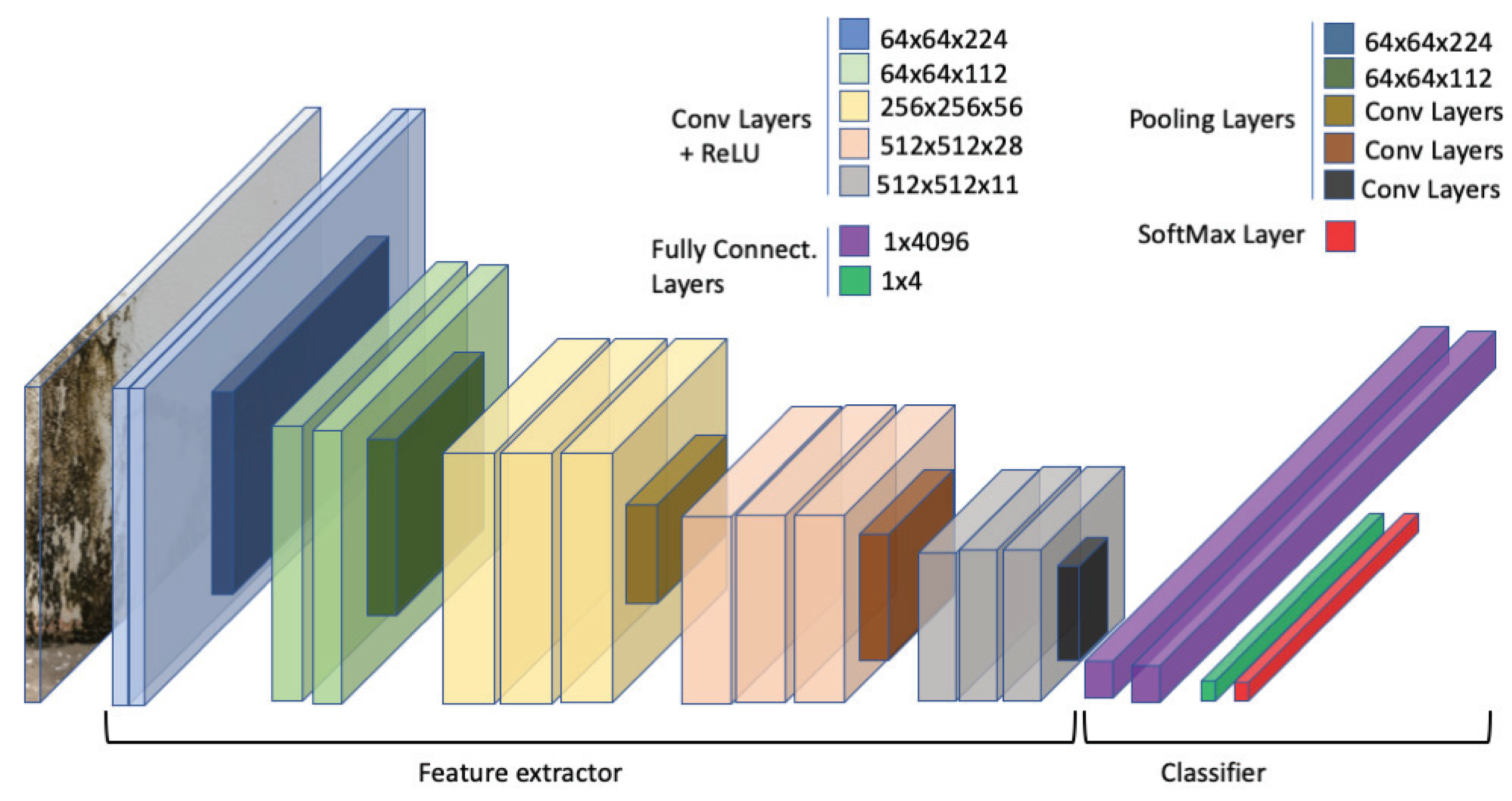
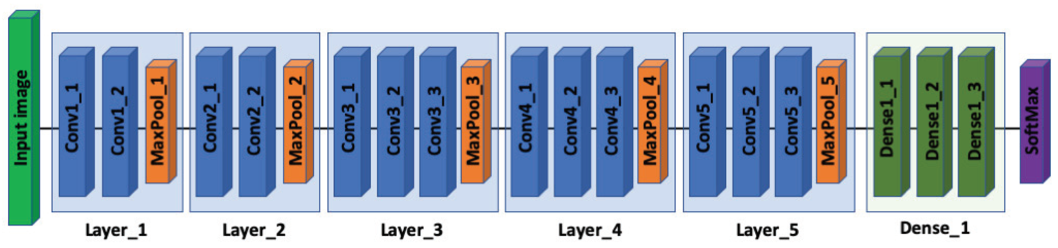
To learn how feature extraction works, one should first understand the architecture of Convolutional Neural Networks (ConvNet). Strictly speaking, most of these network architectures use the same design principles—that is, applying a sequence of convolution layers followed by pooling layers to an input image. Using this structure, the spatial dimensions of each input from previous layers in the network is continuously reduced while the number of features extracted from the input image is increased (see Figure 3).

When extracting features, the fully-connected layers in the pre-trained network are removed and the neural network is treated as a fixed feature extractor. In case of the VGG-16, the fully-connected layers generate 1000 different classes. The earlier layers (convolutional) in the pre-trained network are then trained on the new dataset as feature extractors only. For each input image, the VGG-16 computes a 4096-dimensional feature map. With all feature maps extracted from all the images in the training dataset, a SoftMax classifier with n-classes (the number of classes in the new dataset) may be placed on top of the pre-trained network and trained again on the new dataset.

6. Methodology

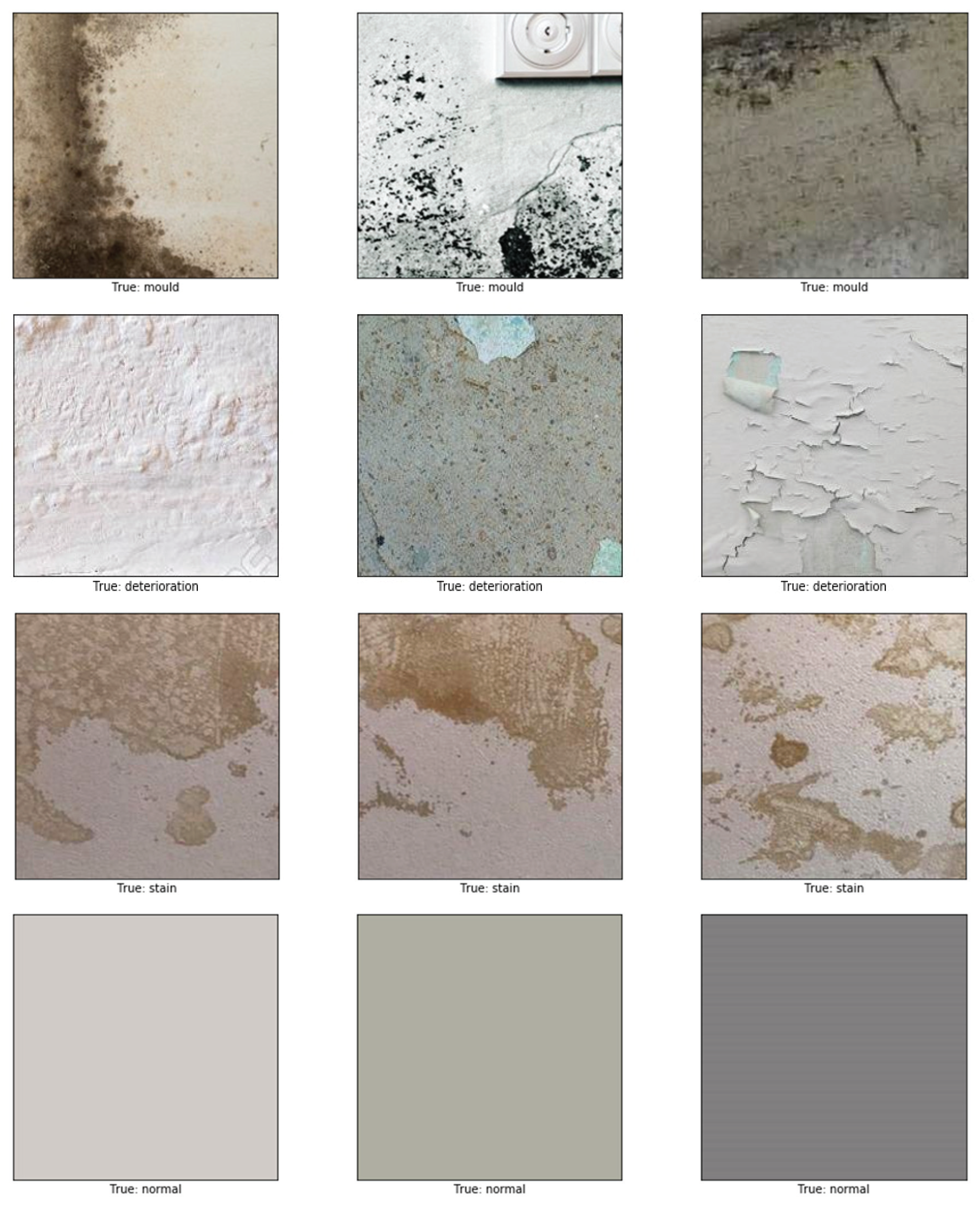
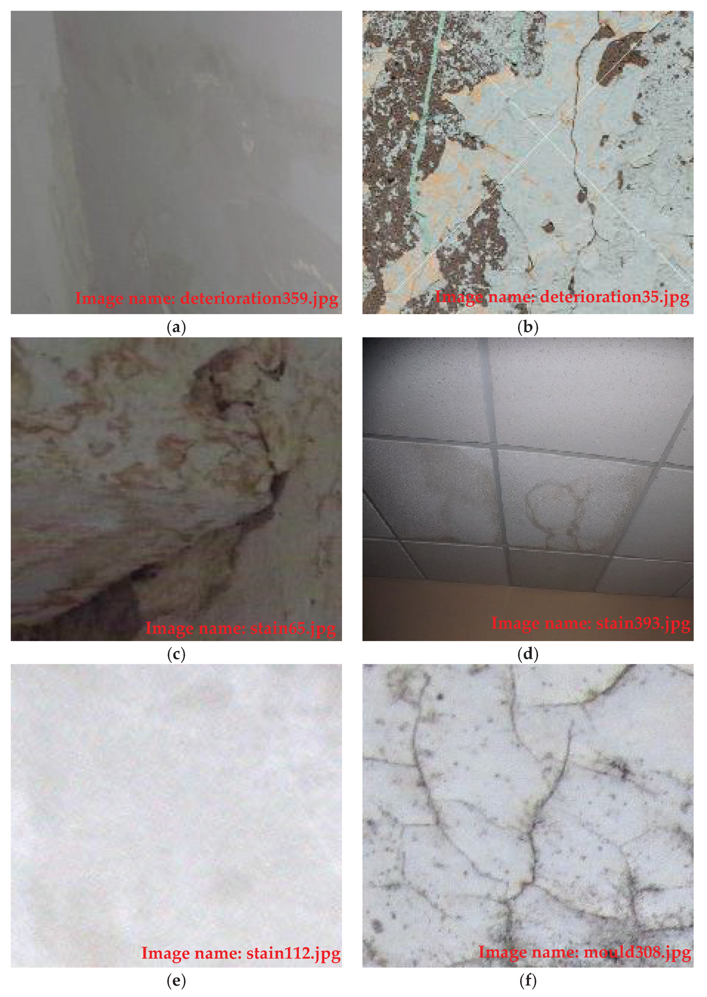
The dataset we used in this research contained images gathered from different resources: pictures taken by mobile phone, by a hand-held camera, and from copyright-free images scraped from the web. In order to increase the number of images in the dataset, the slice tool in Photoshop was used to create 224 × 224 thumbnails out of the large-sized images. In total, the number of images generated for this study was 2523 images. Each image in the dataset was assigned to one of four different classes: normal (image containing no defects), mould, stain, and paint deterioration (this includes peeling, blistering, flacking, and crazing). Assigning images to the right class (labelling) is the most crucial step in supervised machine learning. It is the key to a well-trained model and a high classification accuracy. The dataset was split randomly into 70% (1794 images) for training and the other 20% for testing (validation). The mould class in the training subset contained 448 images, the stain class also contained 448 images, paint deterioration contained 449 images, and, finally, the normal class also contained 449. The validation subset (732 images) was split equally between the four classes with 183 images each. Representative images from the dataset are shown in Figure 4.

The first step in or multistage method is to use the pre-trained VGG-16 model to extract the maps of features of each image in the dataset. The model was developed in Python with the Tensorflow backend. The architecture of the VGG-16 model (illustrated in Figure 4) that we modified comprises five blocks of convolutional layers with max-pooling for feature extraction. The convolutional blocks are followed by three fully-connected layers and a final 1 × 1000 SoftMax layer (classifier). The original SoftMax layer was replaced by a 1 × 4 classifier to adapt our classification problem that is classifying three defects’ types and the normal type. The input to the ConvNet are 224 × 224 RGB images. The first block consists of two convolutional layers with 32 filters, each of size 3 × 3. The second, third, and fourth convolution blocks use filters of sizes 64 × 64 × 3, 128 × 128 × 3, and 256 × 256 × 3, respectively.

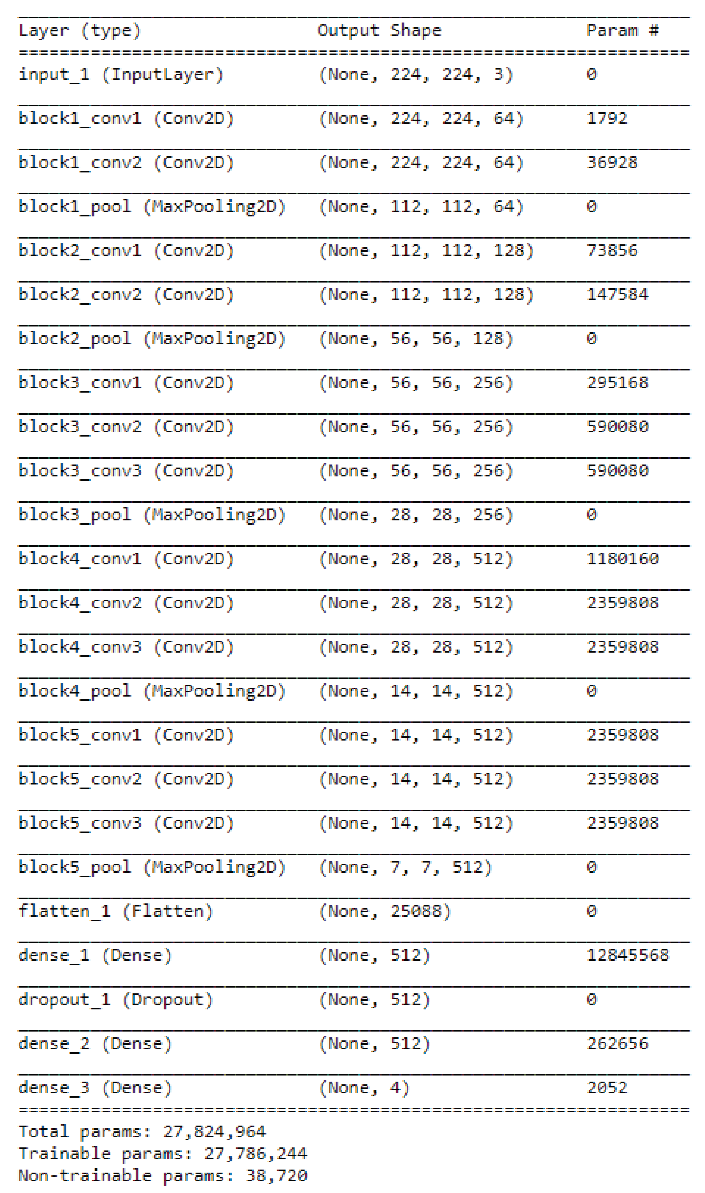
We re-trained the newly modified model on the raw dataset allowing the weights (up to block five) to update during training. We used the early convolutional layers in the VGG-16 (up to the fifth block) as a generic feature extractor. The shape of the input at the last layer of the fifth block is 7 × 7 × 512, as seen in Figure 5. The block is followed by another layer (flatten_1, Figure 6), which, as the name suggests, generates a vector of features of size 25,088. Figure 6 represents a summary of the modified VGG-16 model used in this study.

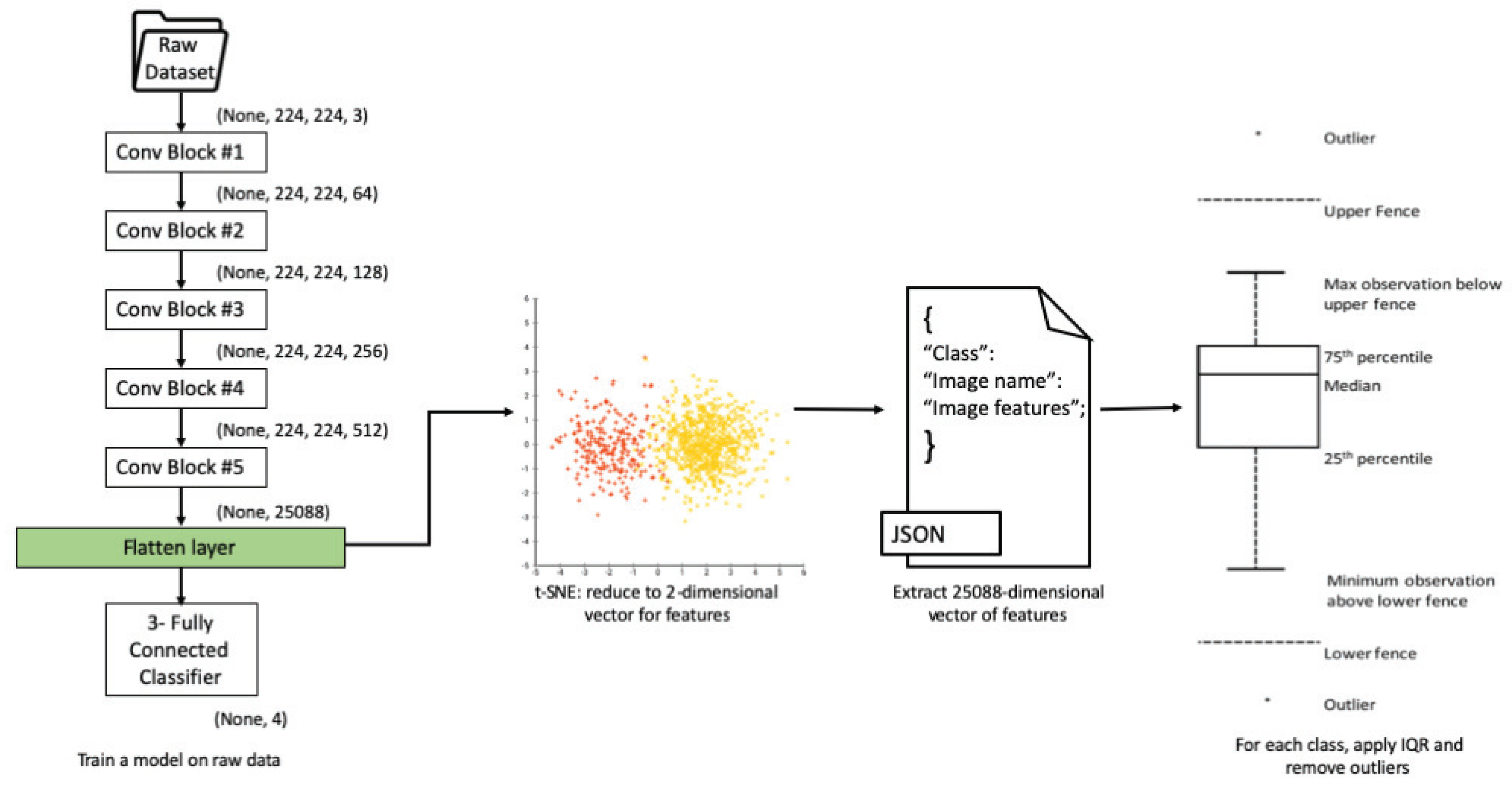
Once all features are extracted from the layer named flatten_1, the second step is the dimensionality reduction. We use t-SNE to reduce the 25,088-dimensions of the extracted vector of features into a map of two dimensions only. t-SNE achieves this by using an iterative approach, making small (sometimes large) adjustments to the mapped points. The process terminates when t-SNE has found a locally optimal (or good enough) embedding. For each image, the newly two-dimensional map can be looked at as a $x$, $y$ position on a plane containing a total number of 2 × $n$ dimensional points, where $n$ is the number of all images in the dataset.

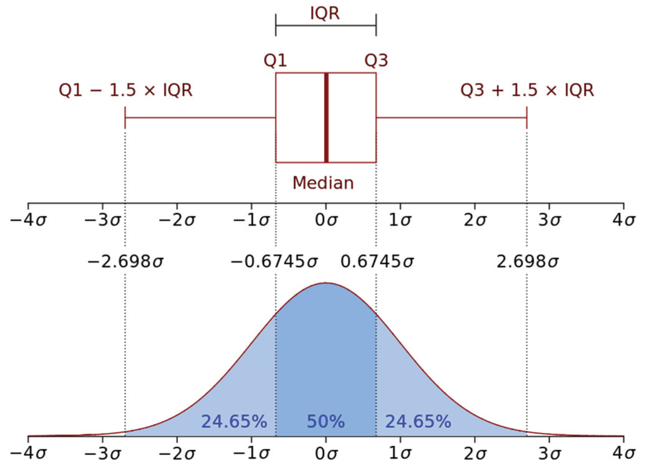
The final step is to use the interquartile range (IQR) on all the points in dimension 1 ($x$–points) and the points in dimension 2 ($y$–points) belonging to all images in every class. For each class of images, any point residing outside the range $[Q_1-1.5\left(Q_3-Q_1\right), Q_3+1.5\left(Q_3-Q_1\right)]$ is regarded as an outlier, and the corresponding image is removed from that class. Figure 7 illustrates the pipeline for identifying outlier images. The block of pseudocode in Algorithm 1 represents the steps for detecting outlier images.

Algorithm 1 Identifying Outlier Images

LoadVGG-16

Read raw dataset

Create function train_vgg16(epochs: real number, data: raw dataset)

Initialize i ←1

While i < epochs do

train VGG-16 on data

End while

Return (features map)

End function

Create function t-SNE(v: features map, dim:2, iter:1000)

Initialisei ← 1

$\sigma =$ variance of the Gaussian

Repeat

For each pair of points $x_i$ and $x_j$ in v do

If $x_i=x_j$ then

$P_{i|i}=0$

Else do

Compute $p_{j|i}=\frac{\exp (-||x_i-x_j|{|}^2/2{{\sigma }_i}^2)}{{\sum }_{k\ne i}\exp (-||x_i-x_j|{|}^2/2{{\sigma }_i}^2)}$

End if

End for

For each counterpart pair of points $y_i$ and $y_j$ in low-dimension do

If $y_i=y_j$ then

$q_{j|i}=0$

Else do

Compute $q_{j|i}=\frac{\exp (-||y_i-y_j|{|}^2)}{{\sum }_{k\ne i}\exp (-||y_i-y_j|{|}^2)}$

End if

End for

i +=

Untili = iter

WriteJSON_file ← class, image_name, $y_i$,$y_j$

return (JSON_file)

End function

Create function IQR(classes:JSON_file)

outliers = [[]

For each class do

For each image_name do

If corresponding $y_i$, and $y_j$ are NOT in $[Q_1-k\left(Q_3-Q_1\right),Q_3+k\left(Q_3-Q_1\right)$ then

Outliers[[] += image_name

Else

Continue

End if

End if

End for

Return (Outliers[[])

End function

Create function Main()

Call train_vgg16()

Call t-SNE()

Call IQR()

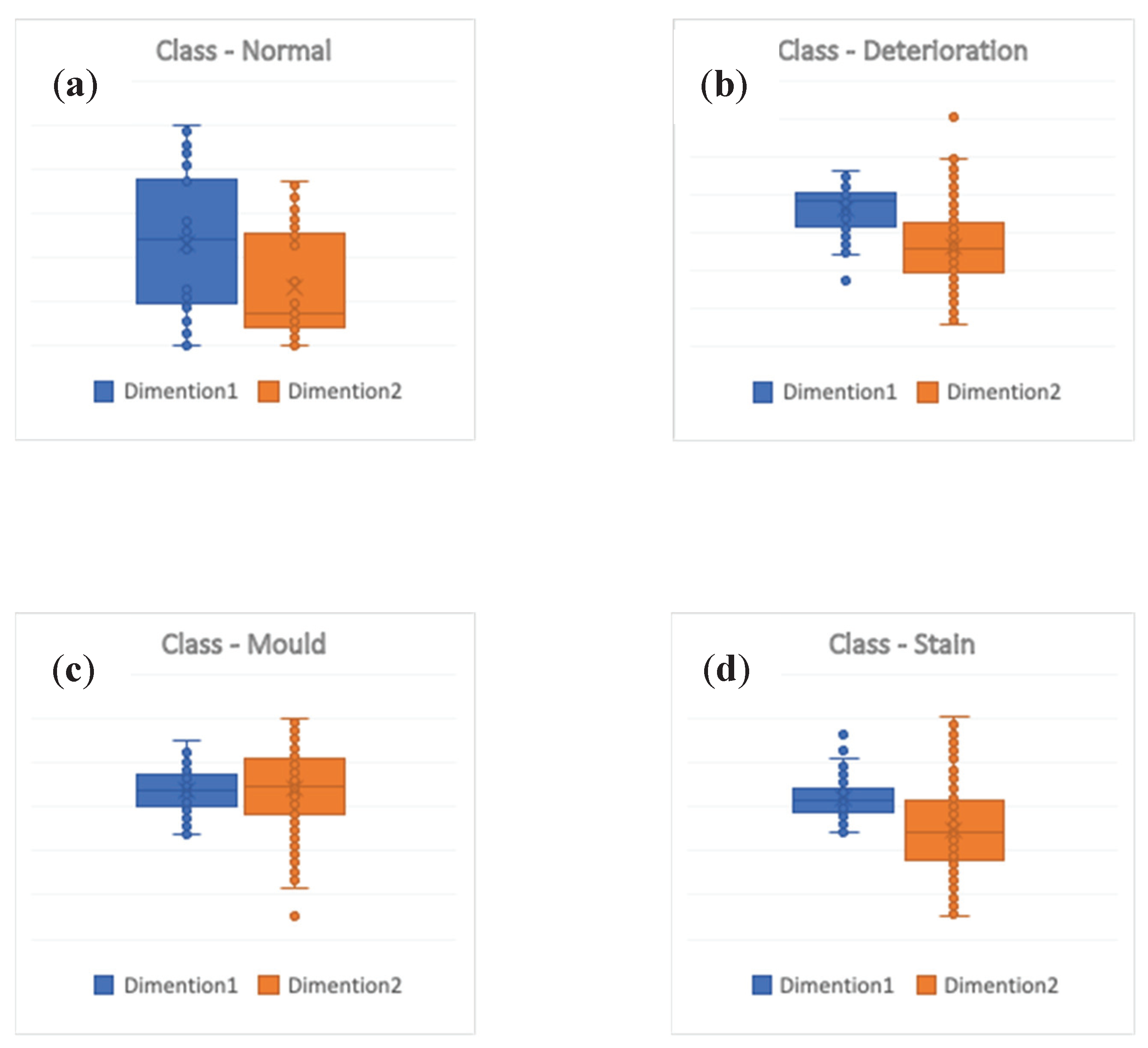
The results of applying the IQR are shown in Figure 8. Figure 8a represents the output of running IQR measure on the class containing images labelled as normal. The boxplot shows no outliers in this class. Figure 8b represents the output of running IQR measure on the class containing images labelled as deterioration. The boxplot shows two outliers in this class. The actual images corresponding to these two outliers are shown in Figure 9a,b. Figure 8c represents the output of running IQR measure on the class containing images labelled as mould. The boxplot shows only one outlier in this class. The corresponding images of this outlier are shown in Figure 9f. Finally, Figure 8d represents the output of running IQR measure on the class containing images labelled as a stain. The boxplot shows three outliers in this class. The corresponding images of the three outliers are shown in Figure 9c–e.

7. Results

To test our model before applying the t-SNE method, we first trained the modified VGG-16 model using the dataset described earlier (over 50 epochs with a batch size of 32 images). After completing the training, the 25,088-dimension vector of features was extracted from the layer (flatten_1) at the end of block eight. All of the information including images names, labels, and extracted features were exported to a JSON file. The classification accuracy was tested using the 732 non-used images mentioned earlier, which are dedicated to evaluating our model. The test accuracy without t-SNE was recorded at 81.25%.

After applying the t-SNE method and removing the outlier images from the dataset, we performed the exact training steps on the same model but using the “cleaned” dataset. We also used the same 732 non-used images dedicated to evaluate the model to test the accuracy. The test accuracy with using t-SNE was recorded at 87.5%.

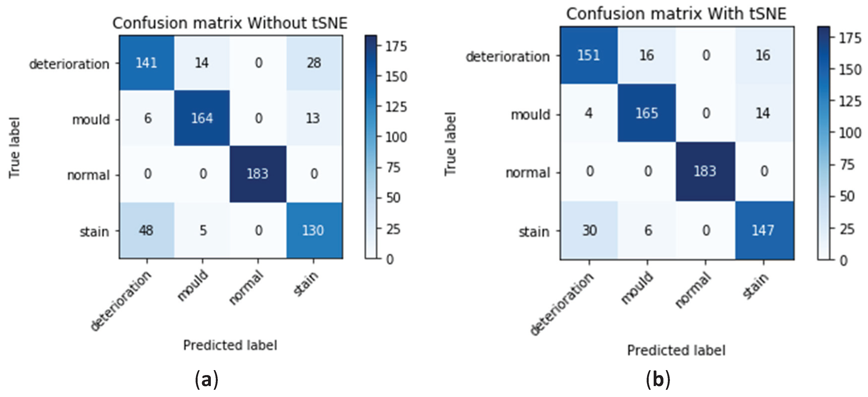
The summary of the performance of the model before applying our method is represented in

Table 1. Accuracy analysis.

	Without t-SNE			With t-SNE
	Precision	Recall	F1-Score	Precision	Recall	F1-Score
Deterioration	0.72	0.77	0.74	0.82	0.82	0.82
Mould	0.89	0.89	0.89	0.89	0.90	0.89
Normal	1.00	1.00	1.00	1.00	1.00	1.00
Stain	0.76	0.71	0.71	0.83	0.80	0.82

(first column) and Figure 10. The confusion matrix is represented in Figure 10a shows that the model has accurately classified 141 out of 183 images containing deterioration with a success rate of around 77%. In this class, the model miss-classified 14 images as mould and another 28 images as stain. For the mould class, the model was able to accurately identify 164 images out of the 183 with a success rate of around 89%. In this class, the model miss-classified six images as deterioration and 13 images as stain. The success rate in the normal class was 100% while, in the stain class, the model was able to accurately classify 130 images only out of the 183 with a success rate of around 71%. In this class, the model miss-classified 48 images as deterioration and five images as mould. The figure also shows that the largest number of miss-classified defects occurs in the stain and deterioration classes. In the analysis summary presented in the first column in Table 1, which corresponds to the performance of the model before applying the method, it can be seen that the overall precision of the model ranges between 72% for detecting deterioration, 89% for mould, 100% for normal images, and 76% for stain. The recall analysis shows similar results, with 77% for detecting deterioration, 89% for mould, 100% for normal, and 71% for stain.

The summary of the performance of the model after applying our method is represented in Figure 10b and Table 1 (second column). The confusion matrix in this figure shows an increase in the number of images containing deterioration accurately classified to 151 out of 183 with a success rate of around 82%. In this class, the model miss-classified 16 images as mould while fewer images (16 images) were miss-classified as stain. For the mould class, a slight increase in the number of images containing mould accurately identified with 165 images out of the 183 resulting in, nearly, the same success rate of around 89%. In this class, the model miss-classified four images only as deterioration and 14 images were miss-classified as stain. The success rate in the normal class remains at 100% while, in the stain class, the model performance has significantly improved by a difference of 17 images. The model was able to accurately classify 147 images out of the 183 giving a significantly higher success rate of around 80%. In this class, only 30 images were miss-classified as deterioration and six images as mould. The figure also shows the significant decrease in the number of miss-classified defects occurring in the stain and deterioration classes with 48 images before applying our model down to 30 after. In the analysis summary presented in the second column in Table 1 which corresponds to the performance of the model after applying the method, improvements in the accuracy can also be seen with an overall precision of the model ranging between 82% for detecting deterioration; nearly no change in the mould class with 89%, 100% for normal images, and, finally, 83% for stain. The recall analysis shows similar results, with 82% for detecting deterioration, 90% for mould, 100% for normal, and 80% for stain.

8. Discussion and Conclusions

In this current work, we proposed a multi-stage method for identifying and removing outliers in image datasets. Outliers, which are defined as extreme values that abnormally lie outside the overall pattern of a distribution of variables, are frequently encountered while collecting data from different resources. In machine learning applications, the presence of outliers in training datasets could significantly compromise the accuracy of the model. Outliers can be of two kinds: univariate and multivariate. Univariate outliers can be found when looking at a distribution of values in a single feature space. Multivariate outliers can be found in an n-dimensional space (of n-features) such as images. We used a dataset with a total of 2532 images to train a modified, by-transfer-learning, VGG-16 model. The same model was also used to generate a vector of features of size 25,088-dimensions. Since handling data distributions in n-dimensional spaces can be challenging for humans, we used a reduction dimensionality technique called t-SNE to create a two-dimensional map of a dataset with images intended to train a ConvNet model. The two-dimensional (dimension1 and dimension2) map of images was analyzed using the IQR measure for detecting any outliers. For each class of images, any point that resides out of the range is outside the range $[Q_1-1.5\left(Q_3-Q_1\right),Q_3+1.5\left(Q_3-Q_1\right)]$ and is regarded as an outlier and removed from that class. The results of applying the IQR showed no outliers in the “Normal” class, two outlier images in the deterioration class, one in the mould class, and three outlier images in the stain class. After removing these images from the dataset, the same model was trained again on the “clean” dataset. We used a dataset with a total of 2532 images to train a modified, by-transfer-learning, VGG-16 model. The model was used to generate a vector of features of size 25,088-dimensions. The model accuracy was then examined using a separate set of 732 images and 183 images for each class. The evaluation test before applying the t-SNE showed a consistent overall accuracy of 81.25%, with 77% of images containing deterioration correctly classified, 89% success rate in detecting images containing mould, a 100% for normal images, and only 71% of images containing stain were correctly detected. The results after applying our method showed that the accuracy has risen significantly from 81.25% before using our method up to 87.5% after applying our method. The improvement in the classification accuracy was noticeable in the stain–deterioration classes where most of the miss-classification originally occurred. The percentage of the images containing deterioration which are accurately detected has increased up 83%, while the success rate in detecting images containing mould and normal remained at 89% and 100%, respectively. The other significant improvement can also be seen in the stain class with an increase in the success rate from 71% up to 80%, with 147 of the images containing stain being correctly detected.

Although using t-SNE can, sometimes, be computationally expensive (when large image datasets are involved), which is one of the disadvantages of dimensionality reductions techniques in general, there are, however, other alternatives, but less accurate than t-SNE such as Principal component analysis (PCA) which may give decent results should high accuracy not be critical. The reason is that PCA only performs linear transformation whilst t-SNE performs the nonlinear transformation. However, PCA can be used in adjunct to t-SNE to help reduce the complexity of high-dimensional transformation, therefore reducing the overall computation time required to perform a complete transformation. In our work, we applied t-SNE over 1000 iterations; however, the number of iterations can be increased to achieve higher accuracy at the cost of the computation time.

We recommend using this technique on raw datasets to improve the quality of the training and testing subsets. This can be particularly useful in applications such as medical imaging, for example, with datasets containing immunofluorescence and immunohistochemistry images, where distinguishing between different types of cells can be quite challenging. In such situations, assigning images to the wrong class is more likely to occur. Applying this technique guarantees that only relevant images are assigned to the right class and outlier images are filtered out.

In our present study, however, we have only studied the effect of removing outlier images from datasets. We have shown that removing images identified as outliers would still improve the overall quality of the dataset, and consequently the accuracy of the model. We believe that further investigation can be conducted on re-assigning the outlier images rather than removing them. One possible way to do this is by using regression techniques such as the K-nearest neighbour algorithm. This is, however, beyond the scope of this research.