Improved Initialization of the EM Algorithm for Mixture Model Parameter Estimation

Abstract

A commonly used tool for estimating the parameters of a mixture model is the Expectation–Maximization (EM) algorithm, which is an iterative procedure that can serve as a maximum-likelihood estimator. The EM algorithm has well-documented drawbacks, such as the need for good initial values and the possibility of being trapped in local optima. Nevertheless, because of its appealing properties, EM plays an important role in estimating the parameters of mixture models. To overcome these initialization problems with EM, in this paper, we propose the Rough-Enhanced-Bayes mixture estimation (REBMIX) algorithm as a more effective initialization algorithm. Three different strategies are derived for dealing with the unknown number of components in the mixture model. These strategies are thoroughly tested on artificial datasets, density–estimation datasets and image–segmentation problems and compared with state-of-the-art initialization methods for the EM. Our proposal shows promising results in terms of clustering and density-estimation performance as well as in terms of computational efficiency. All the improvements are implemented in the rebmix R package.

1. Introduction

The Expectation–Maximization (EM) algorithm was introduced in [1]. Today, after a little more than 40 years, it is still one of the most popular algorithms for statistical pattern recognition. Studies range from the theoretical, i.e., convergence of the EM and its variant DA-EM in [2], to modifications of the EM algorithm for different purposes: image matching [3]; parameter estimation [4,5]; malaria diagnoses [6]; mixture simplification [7]; and audio-visual scene analysis [8].

EM’s popularity has risen due to its use in estimating mixture-model (MM) parameters [9,10]. The mixture model (MM) is an umbrella term for probabilistic models in which the modeled population contains several sub-populations. To describe the characteristics of the sub-population, it is assumed that each sub-population follows a simple parametric distribution, usually referred to as the component of the MM. The type of the MM is therefore identified by the distribution family of its components, e.g., components of the Gaussian Mixture Model (GMM) have a Gaussian distribution. Once estimated, the parameters of MM can be used multi-purposely. Their use is equally interesting for density-estimation tasks [7,11] and clustering tasks [6,12,13]. In the context of MM parameter estimation, the EM algorithm can be seen as a clustering algorithm that maximizes the missing data log-likelihood function as the objective function. Therefore, the EM for MM can be seen as the maximum-likelihood estimator. EM also has many appealing properties, such as monotonic convergence and probabilistic constraints, which makes it appealing in the context of MM parameter estimation.

The EM algorithm also has well-documented drawbacks [14]. It requires some initial parameters for the first iteration. We will refer to this as initialization. The MMs have many parameters, which makes initialization difficult. In addition, EM is very sensitive to initialization. This is because of the multi-modality of the likelihood function for the MM. EM is strictly a hill-climbing algorithm (monotonic convergence property) and therefore can become trapped in local optima. This puts a lot of emphasis on the initialization of the EM algorithm, and there is much research on its initialization (Section 2). Good initialization of the EM algorithm not only improves the results of the estimation problem, but it can also speed up the estimation. The EM algorithm has a linear convergence rate that is characterized as slow [14,15]. However, if the initial parameters are good and close to a saddle point (local optima) of the likelihood function, fewer of the more expensive EM iterations are needed to complete the process.

The initialization of the EM algorithm is a serious problem and should be treated carefully. This is because the initialization creates an additional problem. The number of components in the MM should be known in advance. However, it is usually unknown. Estimating the optimum number of components in the MM is a difficult task [14]. It often fails due to the spurious local optima maximized by the EM algorithm. Estimating the non-optimal number of components in the MM leads to poor performance, either for clustering, density estimation, or any other application of the MM. The best-possible initialization should always be provided in order to avoid such pitfalls.

Therefore, in this paper, we deal with the problem of initializing the EM algorithm for the MM parameter estimation. The initialization uses the Rough-enhanced-Bayes mixture estimation (REBMIX) algorithm [16]. REBMIX is a heuristic for estimating the parameters of the MM that provide a balance between the goodness of the MM parameter estimates and the estimation time [17,18]. In most cases, the parameter estimates with REBMIX are not as good as the ones estimated with the EM algorithm, although the parameter estimates seem to not deviate as much from the parameters estimated with the EM. On other hand, in contrast to the EM, the parameters are estimated quickly. This can be seen in either the REBMIX application to the von-Mises MM parameter estimates in [17] or in the Weibull-Normal MM parameter estimates [18]. Because of this property, we think that REBMIX is a good algorithm for the initialization of the EM algorithm. Although REBMIX can estimate the MM parameters by itself, the need for higher accuracy in a lot of MM applications demands the use of the EM algorithm. The main idea of this paper is that the use of the REBMIX algorithm, as an initialization for the EM algorithm, will result in improved parameter estimates and, therefore, improve the performance in various applications of the MM parameters. In addition to that, due to the fact that REBMIX gives close parameter estimates to the ones of the EM, we believe that the number of iterations of the EM algorithm will be reduced. To prove this, we restrict ourselves to the GMM parameter estimation, being the dominant type of MM and the most troublesome [14]. We propose three different strategies for the GMM estimation, suitable for the model-selection procedures when the number of components in the GMM is unknown. Finally, we conduct a thorough empirical evaluation on the artificial datasets, a density estimation, and image-segmentation tasks. The rest of the paper is structured as follows. Section 2 gives an overview of the relevant work on the initialization of the EM algorithm. Section 3 is the theoretical background for the estimation of the GMM parameters, including the EM, REBMIX, and the coupled REBMIX&EM algorithm. Section 4 gives an overview of the datasets and Section 5 is the results and discussion. The paper ends with Section 6 and the concluding remarks.

2. Related Work

Estimating the MM parameters requires careful initialization of the EM algorithm. In addition, because the EM algorithm needs initialization, two problems emerge. The first is that the complexity parameter of the MM, i.e., the number of components c, must be known (in most cases it is not). Second, even if the number of components c is known, a good set of initial parameters is required to avoid becoming trapped in local optima.

There are two ways to deal with the problem of an unknown number of components c in the MM. Some [13,19,20] initialize the parameters of the MM for the number of components c from the minimum $c_{min}$ to maximum $c_{max}$ number of components and run the EM algorithm on each of them. Then, calculate the goodness-of-fit for each estimated MM with a different number of components and choose the MM that yields the best goodness-of-fit. Others, [12,21,22,23], start by choosing a large number of components c. Then, they initialize the rest of the MM parameters and run the EM algorithm. Finally, they iteratively decrease the number of components c by split&merge and component annihilation techniques until an optimal number of components is found. Although these strategies are sometimes more robust for the initialization of the EM and use fewer EM iterations, they are also lacking. First, they all require criteria for the split&merge and component annihilation techniques and, second, for this strategy to work, the objective function is rewritten to fit the stopping criteria used, such as the, for example, minimum-message-length criterion in [22,23]. This makes any other criteria superfluous. Therefore, we will restrict ourselves to the first strategy, referring to it as model selection. It is worth mentioning that both strategies are deterministic [23]. Stochastic and re-sampling strategies do exist to tackle this problem [9,24] and can be beneficial. However, they are often stand-alone algorithms that do not require EM and/or are often computationally more costly.

The second problem is the initialization of the remaining MM parameters when the number of components c is known. References [14,25] focus on random initialization and provide a lot of useful strategies for EM algorithm initialization. In particular, the strategy called short EM, which repeats a smaller number of iterations of EM with looser convergence criteria on multiple random initializations, of which the one with the highest likelihood is chosen and used to initialize the EM algorithm with more iterations and tighter convergence criteria. Their short EM is also used for the stand-alone initialization procedure explained in [26]. The procedure in [26] was restricted to GMM; hence, additional efforts were made in [27] for different types of MM, which was again based on the short EM strategy. Random initialization of the EM algorithm seems to be an attractive choice for initialization of the EM, as it is used in other papers such as [28,29], or [30], which deal with the initialization problem. Another favorable method for initializing the EM algorithm, but only for the GMM estimation, is the K-means algorithm [26,28,30]. K-means is a clustering algorithm that can be improved with multiple initializations [31] and therefore is useful for initializing the EM for GMM and can give multiple initial parameters. Additionally, K-means initialization tends to provide initial parameters that are closer to final estimates, so fewer EM iterations are needed. Another popular clustering algorithm for initializing the EM for GMM is hierarchical clustering [32]. This initialization technique is purely deterministic. Hence, it cannot be improved by multiple restarts. Although the initializations provided in [32] give close initial parameters to the final estimates and only a few of the EM iterations are needed, the fact that hierarchical clustering is computationally burdensome means that its use for larger datasets is questionable.

Instead of the multiple-repeated random or multiple-repeated k-means initialization, which tends to be used in the literature [14,25,26], here we use the REBMIX algorithm as the initialization technique for the EM algorithm. In contrast to the multiple repeated random or k-means initialization, REBMIX is a purely deterministic algorithm. However, there are other mechanisms that allow the REBMIX algorithm to provide a wide range of initial parameters for the EM algorithm. For this reason, we have tailored three different strategies, which we have called the Exhaustive, the Best and the Single REBMIX&EM Strategy. Each of the three strategies represents how well the parameter space is explored by the REBMIX&EM strategies. The resulting optimized parameter estimates are then used to perform the above-mentioned model-selection procedures and to select the optimum parameters.

3. Estimation of the Gaussian Mixture Model Parameters

Let $\mathit{Y}=\{{\mathit{y}}_1,{\mathit{y}}_2,\cdots ,{\mathit{y}}_n\}$ be an d-dimensional observed dataset of n continuous observations ${\mathit{y}}_j=\{y_1,y_2,\cdots ,y_d\}$. Each observation ${\mathit{y}}_j$ is assumed to follow the probability density function (PDF):

$$f\left({\mathit{y}}_j\right|c,\mathit{w},\mathit{\Theta })=\sum _{l=1}^c{w}_l{f}_l\left({\mathit{y}}_j\right|{\mathit{\Theta }}_l),$$

(1)

where the components have the multivariate Gaussian PDF:

$$f_l\left({\mathit{y}}_j\right|{\mathit{\Theta }}_l)=\frac{1}{\sqrt{{\left(2\pi \right)}^d\mathtt{det}\left({\mathit{\Sigma }}_l\right)}}exp\left(-\frac{1}{2}({\mathit{y}}_j-{\mathit{\mu }}_l.){\mathit{\Sigma }}_l^{-1}{({\mathit{y}}_j-{\mathit{\mu }}_l)}^T\right).$$

(2)

The GMM consists of finite number of components c and every component has weight $w_l$. The weights of the components $w_l$ have the properties of the convex combination $w_l\ge 0\wedge {\sum }_{l=1}^c{w}_l=1$ [9]. Therefore, the estimation of the parameters in the GMM consists of an estimation of the number of components c, an estimation of each component’s weight $w_l$ and each component’s distribution parameters ${\mathit{\Theta }}_l$; in the GMM case, the mean vector ${\mathit{\mu }}_l$ and the covariance matrix ${\mathit{\Sigma }}_l$.

Let $L\left(\mathit{Y}\right|\mathit{\Theta })$ be the likelihood function. The log-likelihood function of the GMM is defined as:

$$logL\left(\mathit{Y}\right|\mathit{\Theta })=\sum _{j=1}^{n}log\left(\sum _{l=1}^c{w}_l{f}_l\left({\mathit{y}}_j\right|{\mathit{\Theta }}_l)\right),$$

(3)

where $f_l\left({\mathit{y}}_j\right|{\mathit{\Theta }}_l)$ is defined in Equation (2). The maximum likelihood estimation of the parameters $\mathit{\Theta }$ can be defined as:

$$\widehat{\mathit{\Theta }}=\underset{\mathit{\Theta }}{argmax}logL\left(\mathit{Y}\right|\mathit{\Theta }).$$

(4)

3.1. Expectation–Maximization Algorithm

The EM algorithm is an iterative algorithm for an estimation of the parameters $\mathit{\Theta }$ of GMM (or any other MM). Instead of maximizing the log-likelihood function for dataset $\mathit{Y}$ containing n observations, it maximizes the complete-data log-likelihood. The complete data ${\mathit{Y}}_c$ is assembled from the observed data $\mathit{Y}$ (sampled dataset) and the missing data (or data labels) $\mathit{Z}$. Missing data are the labels of observations representing the belongings of the observations in the dataset to the components in the GMM. Since the labels of the observations $z_{kj}$ are unknown (for example, the label of the observation ${\mathit{y}}_j$ from the dataset $\mathit{Y}$) the EM algorithm utilizes two steps, i.e., the expectation (E) step and the maximization (M) step. In the E step of the algorithm, the posterior probability ${\tau }_{kj}$ that the observation ${\mathit{y}}_j$ from $\mathit{Y}$ arose from the k-th component is calculated:

$${\tau }_{kj}^{(t+1)}=\frac{w_k^{\left(t\right)}{f}_k\left({\mathit{y}}_j\right|{\mathit{\mu }}_k^{\left(t\right)},{\mathit{\Sigma }}_l^{\left(t\right)})}{{\sum }_{l=1}^c{w}_l^{\left(t\right)}{f}_l\left({\mathit{y}}_j\right|{\mathit{\mu }}_l^{\left(t\right)},{\mathit{\Sigma }}_l^{\left(t\right)})}.$$

(5)

In the M step, the iteration-wise update equations for the parameters can be derived by maximization of conditional expectation of the complete-data log-likelihood function [9]. The updates of the parameters can be obtained with the following equations. The weights $w_k$ with:

$$w_k^{(t+1)}=\frac{{\sum }_{j=1}^n{\tau }_{kj}^{\left(t\right)}}{n},$$

(6)

the mean vectors ${\mathit{\mu }}_k$ with:

$${\mathit{\mu }}_k^{(t+1)}=\frac{{\sum }_{j=1}^n{\tau }_{kj}^{\left(t\right)}{\mathit{y}}_j}{{\sum }_{j=1}^n{\tau }_{kj}^{\left(t\right)}},$$

(7)

and the covariance matrices ${\mathit{\Sigma }}_k$ with update equation:

$${\mathit{\Sigma }}_k^{(t+1)}=\frac{{\sum }_{j=1}^n{\tau }_{kj}^{\left(t\right)}({\mathit{y}}_j-{\mathit{\mu }}_k^{(t+1)}){({\mathit{y}}_j-{\mathit{\mu }}_k^{(t+1)})}^T}{{\sum }_{j=1}^n{\tau }_{kj}^{\left(t\right)}}.$$

(8)

After every successful iteration of the E and M steps, the value of the likelihood is guaranteed to increase [9]. The expectation and maximization steps are repeated iteratively until the convergence of the log-likelihood is achieved. The convergence criteria are mostly assessed by the change in the log-likelihood value, i.e., when it is smaller than some predefined threshold value $\epsilon$ [9,33].

3.1.1. Model Selection with EM Algorithm

Let $\mathit{\Theta }\left(c\right)$ denote the GMM parameters with c components. Let $I=\{{\mathit{\Theta }}_{\mathrm{init}}(c=c_{\min }),{\mathit{\Theta }}_{\mathrm{init}}(c=c_{\min }+1),\cdots ,{\mathit{\Theta }}_{\mathrm{init}}(c=c_{\max })\}$ denote the set of initial parameters of the GMM for the different number of components c. The final set S of estimated parameters becomes $S=\left\{EM\right(i),\forall i\in I\}$, where $EM\left(i\right)$ denotes the iterative process of GMM parameters estimation with the EM algorithm. The problem of model selection can then be summarized as: Choose s from S so that measure $C\left(s\right)$ is optimal, where $C\left(s\right)$ is the cost function for the calculation of the selected measure.

The most commonly used model selection measure, namely information criterion (IC), utilizes the estimated value of likelihood function (or log-likelihood). There is a lot of IC presented in literature, see Chapter 6 of [9]. Out of these, the ones mostly used are definitely AIC and BIC. AIC is defined as:

$$\mathrm{AIC}=-2logL\left(\mathit{Y}\right|\mathit{\Theta }\left(c\right))+2M,$$

(9)

where $M=c-1+cd+cd(d+1)/2$ is the number of parameters in d-dimensional GMM for the number of components c. This criteria mostly favor complex models, due to the small penalization term [25]. Although for most cases of datasets with a larger number of observations n it will select the over-fitted GMM (in terms of number of components c), it is still an interesting criterion for datasets with a smaller number of observations n. The second one, BIC, is defined as:

$$\mathrm{BIC}=-2logL\left(\mathit{Y}\right|\mathit{\Theta }\left(c\right))+Mlogn.$$

(10)

BIC penalizes more heavily complex models than AIC due to the additional multiplicative term of $logn$. On the other hand, for the datasets with a smaller number of observations, it can result in GMM with a very small number of components c (under-fit).

3.2. REBMIX Algorithm

The Rough-Enhanced-Bayes mixture estimation (REBMIX) algorithm is a heuristic approach to the estimation of the GMM [16]. Here, the algorithm will be briefly described. For the interested readers, we advise the following papers [16,34,35]. The algorithm utilizes five simple steps, illustrated in Figure 1. The first step, the preprocessing of observations, conducts an empirical density estimation of the dataset. The empirical density estimation can be carried out in three different ways within the REBMIX algorithm, see ([16], p. 16). However, here the attention is given only to the histogram estimation.

Let v be the number of bins in histogram. The preprocessing step assigns each bin in the histogram a frequency $k_j$, which represents the fraction of the observations falling into the volume $V_j$ occupied by the j-th bin. This is used to transform the input dataset into a new shrunken dataset, consisting only of bin origins ${\overline{\mathit{y}}}_j$ and the corresponding empirical frequency $k_j$ of the bin $j\in \{1,2\cdots v^{*}\}$ (It is worth noting that the $v^{*}$ is the number of non-empty bins of histogram as they are only used for the estimation. Additionally, for convenience, the number of bins v mentioned refer to a one-dimensional histogram. In the multidimensional setting, the actual number of bins is equal to $v^d$, where d is the dimension of the problem). This transformed dataset $\mathit{X}=({\mathit{x}}_1,{\mathit{x}}_2\cdots {\mathit{x}}_j,\cdots {\mathit{x}}_{v^{*}})$, where ${\mathit{x}}_j=({\overline{y}}_1,\cdots ,{\overline{y}}_d,k_j)$, will be denoted as the main cluster. The second step in the algorithm is the global mode detection step. The global mode is simply the mode with highest frequency ${\overline{\mathit{y}}}_m$, where m is defined as $m=\mathrm{argmax}(k_1,k_2,\cdots ,k_{v^{*}})$. The global mode can be always detected and it serves as the basis for the Rough component parameter estimation (Step 3) [16,36]. Rough component parameters are additionally used to split the main cluster $\mathit{X}$ into two clusters, base cluster ${\mathit{X}}_l$, and the residue $\mathit{R}$, where ${\mathit{X}}_l=({\mathit{x}}_{l1},\cdots {\mathit{x}}_{lj},\cdots ,{\mathit{x}}_{lv}^{*})\wedge {\mathit{x}}_{lj}=({\overline{y}}_1,\cdots ,{\overline{y}}_d,k_{lj})$ and $\mathit{R}=({\mathit{R}}_1,\cdots ,{\mathit{R}}_j,\cdots ,{\mathit{R}}_v^{*})\wedge {\mathit{R}}_j=({\overline{y}}_1,\cdots ,{\overline{y}}_d,r_j)$. In addition, the equality $k_j=k_{lj}+r_j,\forall j\in \{1,\cdots ,v^{*}\}$ holds. The base cluster holds the observations tied to the currently estimated component of the GMM and residue is the residual cluster. The split process ends when the criteria $D_l\le D_{\min }/w_l$ is met, where the $D_l$ is sum of positive deviations [16], $w_l$ is the component weight, and $D_{\min }$ is the internally controlled parameter. After the split process is done, the base cluster is used for the Enhanced component parameter estimation. Enhanced component parameter estimates are an approximation of the Gaussian distribution maximum likelihood estimates for the histogram preprocessing [16,36]. The weight of the currently estimated component l is:

$$w_l=\frac{{\sum }_{j=1}^{v^{*}}{k}_{lj}}{n},$$

(11)

the mean vector:

$${\mathit{\mu }}_l=\frac{{\sum }_{j=1}^{v*}{k}_{lj}{\overline{\mathit{y}}}_j}{{\sum }_{j=1}^{v*}{k}_{lj}},$$

(12)

and the covariance matrix:

$${\mathit{\Sigma }}_l=\frac{{\sum }_{j=1}^{v^{*}}{k}_{lj}({\overline{\mathit{y}}}_j-{\mathit{\mu }}_l){({\overline{\mathit{y}}}_j-{\mathit{\mu }}_l)}^T}{{\sum }_{j=1}^{v*}{k}_{lj}}.$$

(13)

The Enhanced component parameter estimation concludes the l-th component parameter estimation. The residue becomes the main cluster, i.e., $\mathit{X}=\mathit{R}$, and the Global mode detection, Rough component parameter, and Enhanced component parameter estimation are repeated to estimate the parameters of a newly added $(l+1)$-th component. This addition of the components ends when the criteria $n_{\mathrm{res}}/n\le c{D}_{\min }$ is met. The $n_{\mathrm{res}}={\sum }_{j=1}^{v*}{r}_j$ is the number of observations in residue and c is the current number of estimated components in GMM. Two intuitive assumptions are made here. The first assumption is the addition of new components should end when the number of observations in the residue is too small to form a new component in the GMM. The control of how small should the residue be is assessed via the parameter $D_{\min }$. The second assumption is that the unassigned observations left in the residue should be redistributed to the already-estimated components and consequently make a certain impact on their parameters. This is made with the Bayes classification of the unassigned observations step [16,36].

The art of the estimation of the parameters of the GMM for the different number of components c lies in updating the parameter $D_{\min }$ iteratively after each Bayes classification of the unassigned observation step is conducted. The parameter $D_{\min }$ is iteratively decreased with the empirical equation $D_{\min }^{\mathrm{new}}=c{D}_{\min }^{\mathrm{old}}/(c+1)$. Parameter $D_{\min }$ is decreased until $c>c_{\max }$. In doing so, the algorithm is forced to iterate until the final set $\{{\mathit{\Theta }}_{\mathrm{final}}(c=1),{\mathit{\Theta }}_{\mathrm{final}}(c=2),\cdots ,{\mathit{\Theta }}_{\mathrm{final}}(c=c_{\max })\}$ of GMM parameters is obtained.

Initially, value of the parameter $D_{\min }$ is taken to be 1. As the weights of the components $w_l$ form a convex combination, the initial value of $D_{\min }=1$ ensures that the first estimated GMM contains only one component. In practice, every decrease in the parameter $D_{\min }$ does not guarantee that estimated GMM will have exactly one more component, or generally speaking more components, as the decreasing equation is empirical. Thus, the set of final estimated parameters of the GMM can be, e.g., $\{{\mathit{\Theta }}_{\mathrm{final}}(c=1),{\mathit{\Theta }}_{\mathrm{final}}(c=2),{\mathit{\Theta }}_{\mathrm{final}}(c=2),{\mathit{\Theta }}_{\mathrm{final}}(c=4)\cdots ,{\mathit{\Theta }}_{\mathrm{final}}(c=c_{\max })\}$. Still, employing different numbers of bins v eases the burden of the above-mentioned problem. In addition, since there is no specific rule to identify v, the presented algorithm flow in [16] runs over an ordered set of numbers K of bins v.

In [16], there is a suggestion to use the same model-selection procedure as described in Section 3.1.1, to select the optimal GMM parameters. However, it is reported in [17,18] that the model-selection procedure usually makes sub-optimal parameter estimates. This happens because the estimated parameters of the GMM with the REBMIX algorithm can be further optimized to yield higher values of the likelihood function (Equation (3)) and therefore provide a beneficial impact on the values of the commonly used IC, for example, BIC, which is defined in Equation (10).

3.3. Combined REBMIX and EM Algorithm

Let R denote the set of solutions (the estimated parameters of the GMM for different numbers of components c) obtained by the REBMIX algorithm. For a certain number of bins v in the histogram preprocessing step and a specified maximum number of components $c_{\max }$ and minimum number of components $c_{\min }$, REBMIX will always provide the same set of solutions R. However, there are many different values for the number of bins v that can be chosen for the preprocessing step. The two extreme cases are the case of $v=1$ and $v=v_{\mathrm{uni}}$, where $v_{\mathrm{uni}}$ is a sufficiently large number of bins for which the $k_j=1,\forall j\in \{1,2,\cdots ,v^{*}\}$ is true. All the values that lie in between these two values can be used for REBMIX to provide different initial parameters for the EM algorithm. As opposed to the stand-alone REBMIX, the use of the EM algorithm ensures that the final estimates yield the maximum likelihood, thus providing more stable grounds for the model-selection procedure. Three different strategies for the coupling of the REBMIX and EM algorithms are proposed. The first strategy, denoted as Exhaustive REBMIX&EM, can be summarized as follows:

• Select the multiple number of bins $v_1,v_2,\cdots$ for histogram preprocessing;
• For each v from $v_1,v_2,\cdots$, obtain the corresponding set of REBMIX estimates $R_{v_1},R_{v_2},\cdots$;
• Merge all solutions from the sets $R_{v_1},R_{v_2},\cdots$ into one set R;
• For each solution $r\in R$, run the EM algorithm and obtain the set S of EM improved estimates of the GMM parameters;
• Run the model selection procedure on the set S.

Although this strategy gives the best potential for the estimation of the parameters of the GMM, it is computationally intensive, due to the many repetitions of the EM algorithm. To ease the computational intensity, the second strategy, denoted as Best REBMIX&EM, is summarized as follows:

• Select the multiple number of bins $v_1,v_2,\cdots$ for histogram preprocessing;
• For each v from $v_1,v_2,\cdots$, obtain the corresponding set of REBMIX estimates $R_{v_1},R_{v_2},\cdots$;
• Group all solutions from the sets $R_{v_1},R_{v_2},\cdots$ by the number of components c, i.e., form the sets $R_{c=c_{\min }},R_{c=c_{\min }+1},\cdots ,R_{c=c_{\max }}$, where each set holds the estimated parameters of the GMM with the same number of components c;
• From each set $R_{c=j}$, choose the solution for which the likelihood value is the largest $r_{c=j,\mathrm{best}}$ and merge it into new set $R_{\mathrm{best}}=\{r_{c=c_{\min },\mathrm{best}},r_{c=c_{\min }+1,\mathrm{best}}\cdots r_{c=c\max ,\mathrm{best}}\}$;
• For each solution $r_{c=j,\mathrm{best}}\in R_{\mathrm{best}}$, run the EM algorithm and obtain the set S of EM improved estimates of the GMM parameters;
• Run the model selection procedure on the set S.

At the end, the least computationally intensive strategy, which additionally minimizes the computation in the REBMIX algorithm, can be derived. This strategy is denoted as the Single REBMIX&EM. If the number of bins v is estimated or intuitively taken as known, the overhead of computing the different parameters $\mathit{\Theta }$ of the GMM for the different numbers of bins v can be reduced in the REBMIX algorithm. This strategy can be summarized as follows:

• Estimate or intuitively select number of bins v;
• Obtain the corresponding set R of REBMIX estimates for known v;
• For each solution $r\in R$ run EM algorithm and obtain the set S of EM estimates of the GMM parameters;
• Run the model selection procedure on the set S.

4. Experiments

The proposed method for estimating the parameters of the GMM was tested on the artificially generated datasets, density estimation tasks, and on the color-image segmentation tasks. Additionally, for a sanity check, two different strategies were included for the EM algorithm: multiple repeated random initialization with the EM algorithm and multiple repeated k-means initialization with the EM algorithm. The number of repetitions of the k-means and the random initialization was 5. They are referred to as the Random&EM and Kmeans&EM. For the model-selection criterion, the BIC was used.

4.1. Artificial Datasets

Artificial datasets were created using the MixSim R package [37]. The utility of this package is in simulating GMMs with various parameters, e.g., with different levels of overlap between the mixture components or number of components (Figure 2). For this research, we have used the dimension of the dataset d, the number of components in the GMM c, and the overlap level a between the components in the GMM.

Table 1. Input parameters used for simulating different Gaussian mixture models.

Parameter	Values
Dimension (d)	3, 5, 10
Number of components (c)	5, 10, 15
Overlap level (a)	0.001, 0.125

summarizes the input parameters. Using all the combinations of input parameters, 18 different parameters of GMMs were simulated. Sampling of the datasets from each simulated GMM was done with $n=100$, $n=1000$, and $n=$ 10,000 observations, which resulted in 54 different datasets.

4.2. Density Estimation

To study the performance of the proposed strategies for the density estimation, we chose the multivariate distributions presented in [11], for which their implementation performed well. The distributions are: Trips-2d, Blob 2-d, Bend 2-d, Wave 2-d, Trips 3-d, Blob 3-d, Bend 3-d, Spiral 3-d, and Tetra 3-d, where 2-d and 3-d represent the dimension of the distribution. The datasets were sampled with different number of observations $n=50,100,200,300,400,500,750,1000,1500$. The number of replications of each dataset was 10. For the performance measure of the density estimates, we have chosen the same measure as in the original paper, the mean integrated square error (MISE) between the true density and estimated density. MISE is defined as:

$$\mathrm{MISE}=\frac{1}{r}\sum _{i=1}^r\int {(f\left(\mathit{y}\right)-\widehat{f}\left(\mathit{y}\right))}^{2}d\mathit{y},$$

(14)

where r is the number of replications, $\widehat{f}\left(\mathit{y}\right)$ estimated density, and $f\left(\mathit{y}\right)$ the true density. Additionally, Reference [11] provides an R implementation of their work, so we included the results obtained with their Adaptive density estimation by Bayesian averaging (ADEBA) algorithm.

4.3. Image Segmentation

To study the performance of proposed strategies for the clustering, we have selected the digital-image segmentation task. The digital-image-segmentation task can be seen as a real-world clustering problem. To elaborate, segmentation of an image means grouping, i.e., clustering, the image into coherent parts. The pixels in the digital image hold certain values of color intensity (brightness). In general, color digital images are represented by three channels, where each channel holds the intensity of one primary color, such as red, green, and blue (known as RGB images). The clustering problem in this setting can be conceived as color quantification of the digital image or, more simply, grouping the parts of the digital image by the color similarity. Hence, the use of GMMs for this is appropriate. The estimation and the model selection are carried on all the pixel color values in the digital image. Once the GMM parameters are estimated, the clustering scheme can be obtained by assigning each pixel $j\in \{1,\cdots ,n\}$ in a given image with n pixels to the one of the components in the estimated GMM. The assignment is made with the posterior probabilities ${\tau }_{lj}$, namely the component for which the posterior probability is highest $l=\mathrm{argmax}({\tau }_{1j},{\tau }_{2j},\cdots ,{\tau }_{cj})$ [33]. Posterior probabilities ${\tau }_{lj}$ for pixel j are obtained using Equation (5). The number of clusters, therefore, becomes the number of components c in estimated GMM.

The clustering performance is assessed through the Adjusted Rand Index (ARI) measure [38]. To define the ARI, first we need to define the contingency table (

Table 2. Contingency table.

M/N	${\mathit{N}}_1{\mathit{N}}_2\cdots {\mathit{N}}_{\mathit{s}}$	Sums
$M_1$	$n_{11}{n}_{12}\cdots n_{1s}$	$a_1$
$M_2$	$n_{21}{n}_{22}\cdots n_{2s}$	$a_2$
⋮	$⋮⋮\ddots ⋮$	⋮
$M_r$	$n_{r1}{n}_{r2}\cdots n_{rs}$	$a_r$
Sums	$b_1{b}_2\cdots b_s$

). The contingency table is used to summarize the overlap between the two clustering schemes $M=\{M_1,M_2,\cdots ,M_r\}$ and $N=\{N_1,N_2,\cdots ,N_s\}$ with different numbers of clusters r and s. Each entry $n_{ij}$ in the contingency table represents the common number of objects in clusters i and j, respectively, from the M and N clustering schemes.

ARI is defined as:

$$ARI=\frac{{\sum }_i^r{\sum }_j^s\left(\genfrac{}{}{0pt}{}{n_{ij}}{2}\right)-[{\sum }_i^r\left(\genfrac{}{}{0pt}{}{a_i}{2}\right){\sum }_j^s\left(\genfrac{}{}{0pt}{}{b_j}{2}\right)]/\left(\genfrac{}{}{0pt}{}{n}{2}\right)}{\frac{1}{2}[{\sum }_i^r\left(\genfrac{}{}{0pt}{}{a_i}{2}\right)+{\sum }_j^s\left(\genfrac{}{}{0pt}{}{b_j}{2}\right)]-[{\sum }_i^r\left(\genfrac{}{}{0pt}{}{a_i}{2}\right){\sum }_j^s\left(\genfrac{}{}{0pt}{}{b_j}{2}\right)]/\left(\genfrac{}{}{0pt}{}{n}{2}\right)},$$

(15)

where $n_{ij}$, $a_i$, $b_j$ can be acquired from the contingency table. The ARI is bounded between −1 and 1, where 1 means that the two clustering schemes have 100% agreement and a negative ARI value means that the agreement is not better than the random. Therefore, the higher the ARI value, the better the match between the two clustering schemes.

For the image-segmentation tasks, five images from the famous Berkeley dataset were used [39], see Figure 3. The images additionally have human segmentation, which can serve as a ground-truth segmentation for the evaluation of the performance of the clustering. As reported in [39], each image in the dataset has multiple human segmentations and they are all considered valid. Therefore, the ARI is calculated for each human segmentation and the maximum value is reported.

5. Results and Discussion

5.1. Results on Artificially Generated Datasets

First, let us introduce the parameters used for the proposed strategies. The Exhaustive REBMIX&EM and Best REBMIX&EM strategies require an ordered set of the numbers of bins K, and the Single REBMIX&EM strategy requires a single number of bins v as the input. The ordered set of the numbers of bins K had 3–100 bins. For the Single REBMIX&EM strategy, the number of bins v was estimated using the Knuth rule [40]. The maximum number of components $c_{\max }=20$ and the minimum numbers of components $c_{\min }=1$ is kept the same for every strategy, along with the Kmeans&EM and the Random&EM. The threshold value for the average log-likelihood value (for the convergence assumption) was $0.0001$ and the maximum number of EM iterations allowed was 1000. The choice of convergence of the EM with the average log-likelihood value was made because it removes the impact of larger and smaller datasets (in terms of the number of observations). The average log-likelihood was calculated simply by dividing the log-likelihood value $L\left(\mathit{y}\right|\mathit{\Theta })$ by the number of observations n in the dataset.

Secondly, let us describe the methodology used to compare the strategies here. As explained in Section 3.1.1, the purpose of the model-selection procedure is to choose the appropriate GMM parameters based on the defined measure, which was in our case BIC. Therefore, the quality of the estimated GMM parameters can be expressed by the corresponding value of the BIC. If the strategy estimated the GMM parameters that gave the best value of the BIC, i.e., the lowest value compared to other strategies used, then we assume that the strategy also estimated the best GMM parameters. This is a reasonable and commonly used method for comparing the quality of the estimated GMM parameters [14,32]. In addition, the use of the MixSim R package to sample the artificial datasets (Section 4.1) allows the true density estimation and the clustering for each artificial dataset to be determined based on the fact that the GMM from which the data set was sampled is known. This was used to additionally compare the clustering (Section 5.1.1) and density-estimation (Section 5.1.2) performance of the estimated GMM parameters.

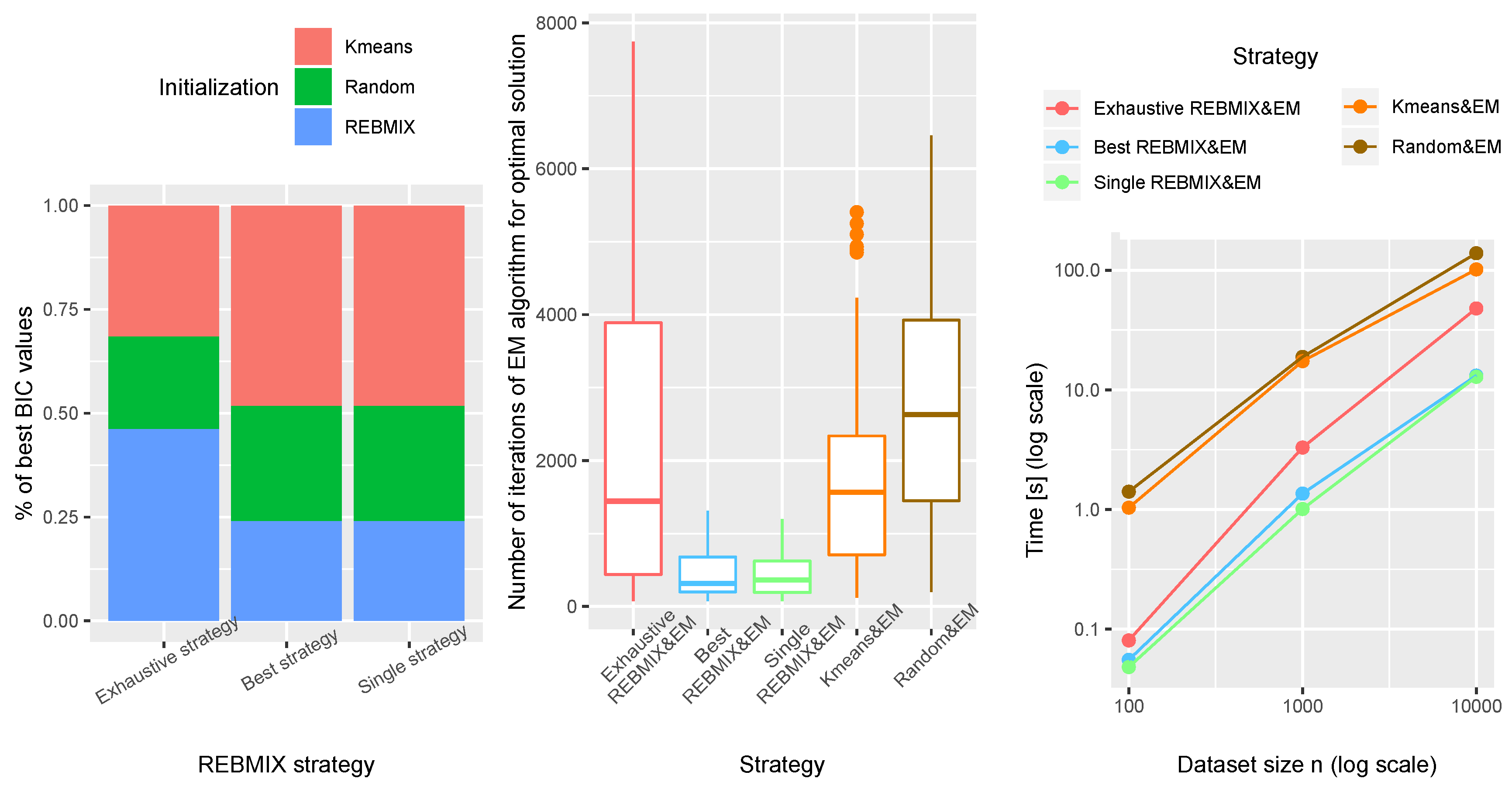
The general results are presented in Figure 4 which are acquired on all artificial datasets. The first plot represents the percentage of selected GMM with the best BIC value for each REBMIX&EM strategy versus the Kmeans&EM and Random&EM strategy. Exhaustive REBMIX&EM selected better GMM on more datasets than Kmeans&EM and Random&EM strategy, judging by the BIC value. On other hand, strategies Best and Single REBMIX&EM had a smaller number of datasets on which they yielded best GMM in terms of BIC value than Kmeans&EM and equal to the Random&EM strategy. The second plot represents the box-plots of the EM iterations used by each strategy. The Random&EM strategy needed the largest number of EM iterations. Following this is the Exhaustive REBMIX&EM strategy, then the Kmeans&EM strategy, and the smallest number of iterations was needed by the Best and Single REBMIX&EM strategies. This is inferred based on the median value of the box-plots (horizontal line inside the box). In addition, the Best and Single REBMIX&EM strategies had a much smaller number of iterations of the EM algorithm, due to the fact that they had only one set of initial parameters for each number of components $c=1,2,3\cdots 20$, as opposed to, e.g., the Random&EM, which had five sets of initial parameters for each number of components. However, interestingly, the Exhaustive REBMIX&EM strategy had at least 90 different sets of initial parameters for each number of components and still had a smaller number of iterations than the Random&EM and had the same median value as the distribution of the number of iterations for the Kmeans&EM. That does seem to be beneficial to the REBMIX algorithm, which seems to provide very close to the initial parameters of the GMM to the final estimated parameters. Finally, the third plot shows the amount of time spent on estimating the GMM parameters with different strategies. The Best and Single REBMIX&EM strategies had similar computing times and therefore their effectiveness seems to be equivalent. Most of the differences in the performance of these two strategies stem from the fact that the Best REBMIX&EM strategy had a multiple number of bins v (3–100) for the REBMIX algorithm, as opposed to the Single REBMIX&EM strategy, for which we used the Knuth rule to obtain the single number of bins v. Moving forward, the Exhaustive REBMIX&EM strategy gradually increased the required computation time with the increase in the number of observations. This is to be expected, since this strategy required the most EM iterations (second plot) compared to the other two REBMIX&EM strategies. The Random&EM and Kmeans&EM strategy had the worst performance in terms of the computing time. Although the Random&EM strategy needed less time when the number of observations was lower, the Kmeans&EM strategy outperformed it as the number of observations increased. Judging by the actual values, however, the difference between these two strategies was not great.

5.1.1. Application to Clustering

The ARI is used to study the clustering performance. The results are given as box-plots in Figure 5. The grouping in Figure 5 was selected because it reflects the difficulty of the dataset, i.e., a small number of observations in the dataset along with a high degree of overlap between the components can be seen as a difficult clustering problem, while the large number of observations with a small degree of overlap can be seen as a simpler clustering problem.

The performance of the Exhaustive REBMIX&EM strategy and the Best REBMIX&EM strategy on smaller datasets ($n=100$) with a lower degree of overlap was better than the multiple repeated Kmeans&EM and multiple repeated Random&EM strategy. The Kmeans&EM strategy improved the results for the datasets with a larger number of observations with smaller overlap although the Exhaustive REBMIX&EM strategy and the Best REBMIX&EM strategy performed equivalently or better. The Random&EM only had equivalent results on the largest datasets n = 10,000. The Single REBMIX&EM performed slightly worse than the Exhaustive REBMIX&EM strategy and the Best REBMIX&EM strategy, although equivalently to the Kmeans&EM strategy and mostly better than the Random&EM strategy. On the other hand, the datasets with larger overlap reduced the clustering performance of all the strategies, especially for datasets with $n=100$ and $n=1000$. In this context, the Kmeans&EM performed better than all the REBMIX&EM strategies for datasets with a small number of observations $n=100$. On datasets with a larger number of observations $n=1000$ only the Exhaustive REBMIX&EM strategy performed as well as the Kmeans&EM strategy, while only the Random&EM strategy performed poorly. On the datasets with the largest number of observations n = 10,000, the strategies Exhaustive and Best REBMIX&EM slightly outperformed the other strategies. We have also included the results we obtained just by running the REBMIX algorithm. For the K, we chose the 3–100 range—in other words, the same as for the Exhaustive and Best REBMIX&EM strategy. The results for the $n=100$ were mainly worse than the results from all the other strategies. As this number increased, i.e., $n=1000$ and n = 10,000, the performance improved, although the other strategies still performed better.

5.1.2. Application to the Density Estimation

To study the performance of the estimated GMM with different strategies in terms of density estimation, we used the mean square error (MSE) measure [33]. The MSE is defined as:

$$\mathrm{MSE}=\frac{1}{N}\sum _j^n{(f\left({\mathit{y}}_j\right|\widehat{\mathit{\Theta }})-f\left({\mathit{y}}_j\right|\mathit{\Theta }))}^2,$$

(16)

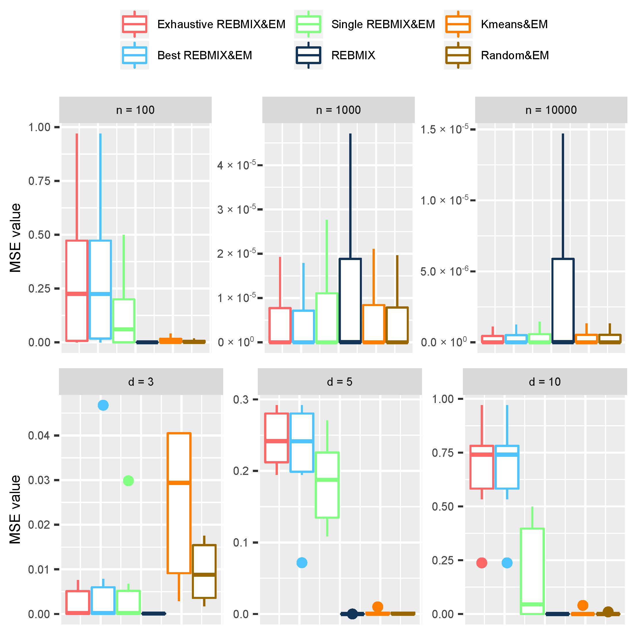
where $\widehat{\mathit{\Theta }}$ are estimated GMM parameters with different strategies and $\mathit{\Theta }$ are the true GMM parameters from simulation. The choice of MSE instead of MISE was made here because the distributions used for sampling the datasets had higher dimensions, i.e., 3, 5, and 10, and the creation of the good integration grid requires a lot of computing power in terms of memory. The results are therefore presented as box-plots of MSE values in the upper plot in Figure 6. These box-plots are grouped by the number of observations in the dataset. Again, for the estimation, we have used all the strategies and the stand-alone REBMIX algorithm.

Judging by the values presented, all the strategies and the stand-alone REBMIX gave good results for the datasets with $n=1000$ and $n=10000$. In contrast, for $n=100$, the Kmeans&EM, Random&EM, and REBMIX had much better results than the REBMIX&EM strategies. To study more carefully why this happened, the box-plots for the datasets with $n=100$ observations only are given in the lower plot (Figure 6), grouped by the number of dimensions d in the dataset. It is clear that, as the dimensionality of the dataset increased, the results became worse. Although the stand-alone REBMIX algorithm had good results, it is clear that the results of the REBMIX&EM strategies deteriorated. To understand why this happened, we must recall that the log-likelihood function, defined in Equation (3), for the GMM is unbounded. Namely, a singularity in one of the component covariance matrices ${\mathit{\Sigma }}_l$ can arise when $det\left({\mathit{\Sigma }}_l\right)\to 0$ [33]. When this problem appears, the EM can be jeopardized and the obtained solution can degenerate. A high-dimensional setting, such as $d=5$ or $d=10$, emphasizes this problem even more [14]. Because we did not include any of the safeguards for the EM algorithm, in terms of bounding the log-likelihood function, the resulting log-likelihood increased and the model-selection procedure was misled into choosing the degenerated solution.

5.2. Density-Estimation Tasks

For the density estimates, the same parameters were used for the three REBMIX&EM strategies as in the case of the Artificial datasets and also the same for the Random&EM and Kmeans&EM strategies. For the ADEBA algorithm, we used the parameters for the ADEBA −$\alpha$ implementation (see [11], Section 3), i.e., the parameter $\alpha$ is chosen with Bayesian averaging and $\beta =1$ for which we will use the generic term ADEBA.

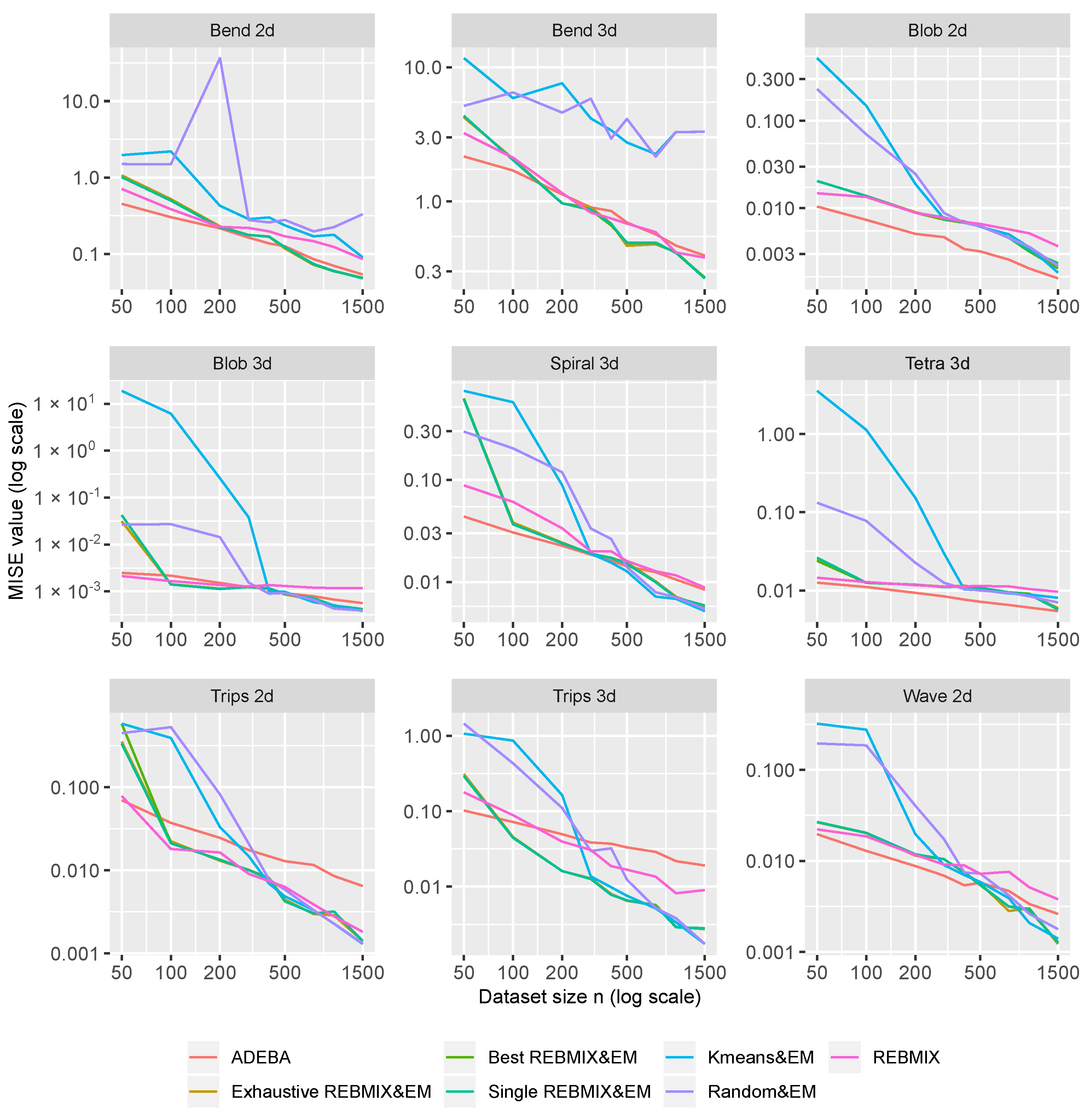
The acquired values of MISE for each pair of strategy/method and distribution are shown on different plots in Figure 7. In general, the GMM estimates using different strategies yielded better results with an increase in the dataset size n. For the small dataset sizes, e.g., $n=50$ and $n=100$, ADEBA usually had the best results, although the REBMIX&EM strategies proved to be good competitors, which can be seen from the results on the distributions Bend 2-d, Bend 3-d, Trips-2d, Blob 2-d, Tetra 3-d and Wave 2-d. For the datasets sampled from the distributions Trips-2d and Trips-3d with an increasing size of the dataset, all the strategies used outperformed the ADEBA. This is expected because the Trips-2d and Trips-3d distributions are actually GMM distributions with $c=3$ non-overlapping components. Interestingly, the ADEBA outperformed all the strategies used for all the dataset sizes n on the Blob 2-d distribution, which is also a GMM distribution with $c=8$ overlapping components. However, as the dimension of the distribution increased (i.e., the distribution Blob 3-d is only the same distribution as Blob 2-d in three-dimensional space), the results from the ADEBA deteriorated. On the distributions Bend 2-d and Bend 3-d, all the estimators had their performance deteriorated. Kmeans&EM and Random&EM performed worse than the REBMIX&EM strategies and the ADEBA. On the Spiral 3-d distribution for the $n=50$ REBMIX&EM strategies, the Kmeans&EM and Random&EM strategy performed worse than the ADEBA, although their performance improved as the n increased (for the REBMIX&EM strategies again from $n=100$ and and for the Kmeans&EM and Random&EM strategies from the $n=300$ and $n=500$, respectively). For the distributions Tetra 3-d and Wave 2-d, the results are similar to the ones for the Blob 2-d distribution. Between the different REBMIX&EM strategies, the results did not differ greatly. The slight difference can be seen on the smaller dataset sizes n. However, as n increased, the results were almost identical. We have also evaluated REBMIX, as a stand-alone algorithm, for this experiment. Again, K was 3–100. REBMIX was better when the number of observations in the dataset was small, usually only for $n=50$. On other hand, just the increase from the $n=50$ to $n=100$ improved the results from the REBMIX&EM strategies on many distributions, most notably on the GMM distributions such as Trips 3d.

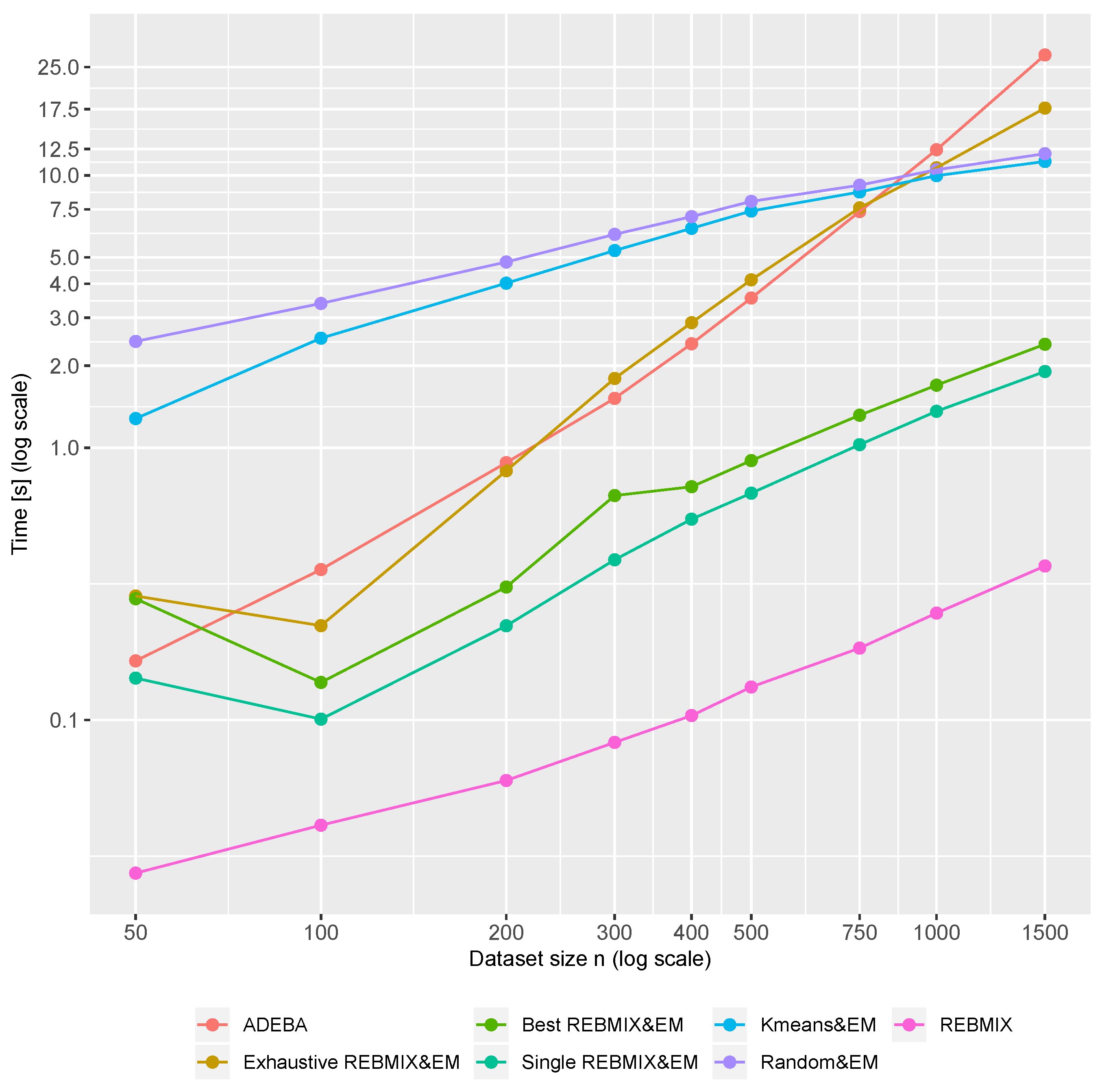
To study the performance of different EM strategies and the ADEBA, the computation times for each method/strategy were measured for different distributions and different dataset sizes n. The values are grouped by the dataset size n and the method/strategy, and the mean values are shown in Figure 8. The Single and Best REBMIX&EM strategy far outperformed all the other strategies used and the ADEBA algorithm for all the dataset sizes, with the exception of size $n=50$, where the ADEBA and REBMIX&EM strategies achieved equivalent results. The Exhaustive REBMIX&EM strategy performed as well as the ADEBA. The Kmeans&EM and Random&EM performed worse on all the dataset sizes, with the exception of the dataset size $n=1500$, where they performed slightly better than the ADEBA and Exhaustive REBMIX&EM. The REBMIX stand-alone outperformed all the used strategies and the ADEBA algorithm in terms of computation efficacy.

5.3. Image-Segmentation Tasks

The image segmentations were carried out using the following strategies: the Single REBMIX&EM strategy, where the number of bins v was estimated using the Knuth rule; the Single REBMIX&EM strategy, where the number of bins v was taken to be $v=255$; the Best REBMIX&EM strategy, with the range of the number of bins being 3–100; and the Kmeans&EM strategy and the Random&EM strategy. The number of bins $v=255$ was taken as the color-channel value. The intensities of the RGB images only have integer values and, therefore, the frequency of each color channel is estimated. Furthermore, using $v=255$, the marginal distributions of the color-channel value’s intensity are represented. The maximum number of components for each strategy is kept the same, i.e., $\mathtt{cmax}=20$. The threshold value for the EM algorithm was $0.0001$ and the maximum allowed number of EM iterations was 1000.

The numerical results in terms of the number of components c and the ARI value are given in

Table 3. Numerical results of image segmentation tasks.

Image Label/Strategy		353013	38092	216053	48055	22093
Random&EM	c	20	20	20	20	20
	ARI	0.29	0.28	0.47	0.37	0.34
Kmeans&EM	c	20	20	20	20	20
	ARI	0.24	0.28	0.24	0.36	0.35
Single REBMIX&EM with Knuth rule	c	20	19	19	19	20
	ARI	0.38	0.42	0.35	0.41	0.41
Single REBMIX&EM with $v=255$	c	18	20	20	20	20
	ARI	0.67	0.67	0.63	0.45	0.34
Best REBMIX&EM	c	19	16	16	16	18
	ARI	0.44	0.54	0.25	0.47	0.38

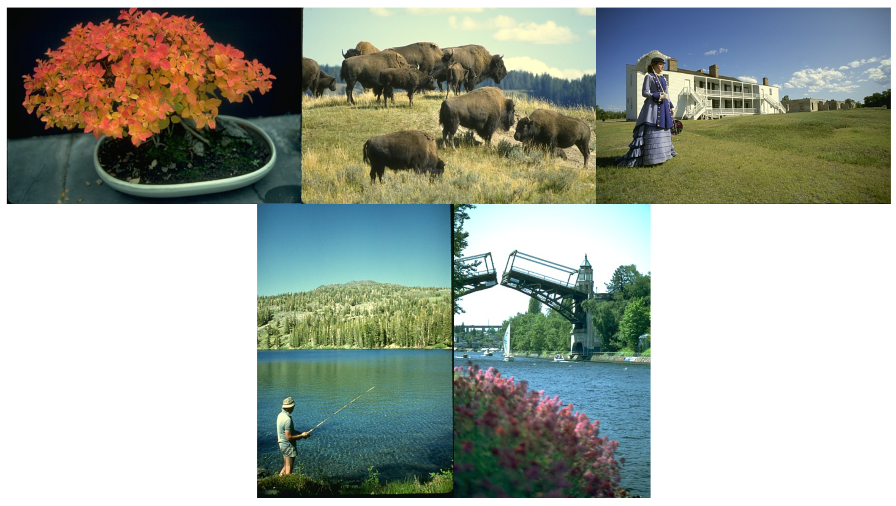
. From the numerical results, one of the REBMIX&EM strategies always had the best ARI values. Additionally, the Single REBMIX&EM with $v=255$ yielded very good results in terms of ARI value on the flower image (353013), herd image (38092), and woman image (216053); therefore, the intuitive guess of $v=255$ was shown to be beneficial. Finally, the selected GMMs with all strategies had a large number of components c, which can be related to the BIC model selection criteria.

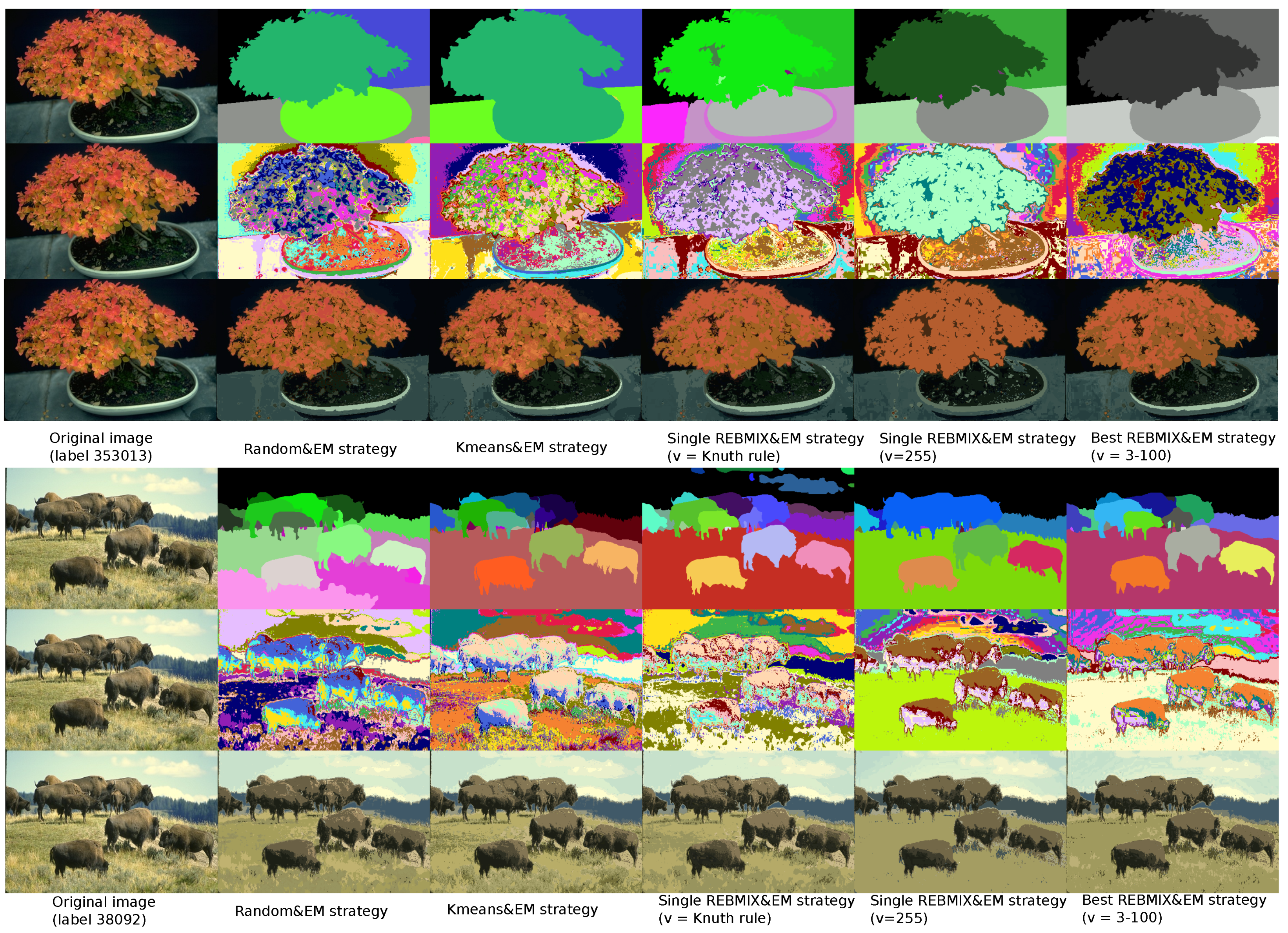
To establish some qualitative comparison, the segmentations of the flower and herd images are given in Figure 9. First, the issue of the black or white colored background. Namely, the black or white colored background caused a high density on the edges of the feature space, creating a heavy-tailed distribution, for which GMMs are not suitable. The GMMs estimated with each strategy needed at least two components to address the heavy tails of distribution; therefore, a background like on the flower image (label 353013) was mostly over-segmented and caused a lower ARI value. Next, the strategies mostly had problems with the objects that occupied a large part of the image scene and had little variation in color (for example, the flower object on the flower image or soil on the herd image). Namely, the object that occupied larger parts of the scene caused a high-density peak in the distribution. This high-density peak caused a certain asymmetry in the distribution and the strategies tried to fit multiple components of the GMM for that part. This caused a lot of noise in the segmentation, which can be seen in Figure 9. This problem was slightly reduced by the Single REBMIX&EM strategy with $v=255$, which mostly did tie the peaks with one component of the GMM (flower object in the flower image or the soil-ground part of the herd image in Figure 9). This also led to a much higher ARI value for those segmentations. The sky gradients mostly caused over-segmentations, which were not properly addressed by any strategy.

Additionally, we also included results from purely clustering algorithms, such as the MeanShift (MS) algorithm or the newer Cutting edge spatial clustering (CutESC) [41], which exhibited good results in their study. We have used scikit-learn Python MS implementation [42] with default values. The segmentation was made on the original pixel-color values. For the CutESC algorithm, we followed their recommendation. First, we calculated superpixels of the images with scikit-image SLIC implementation [43] with defaults values and then constructed a shrunken dataset, containing the spatial and color values.

Table 4. ARI values obtained from MS and CutESC clustering algorithm.

Image/Algorithm	353013	38092	216053	48055	22093
MS	0.46	0.54	0.69	0.1	0.43
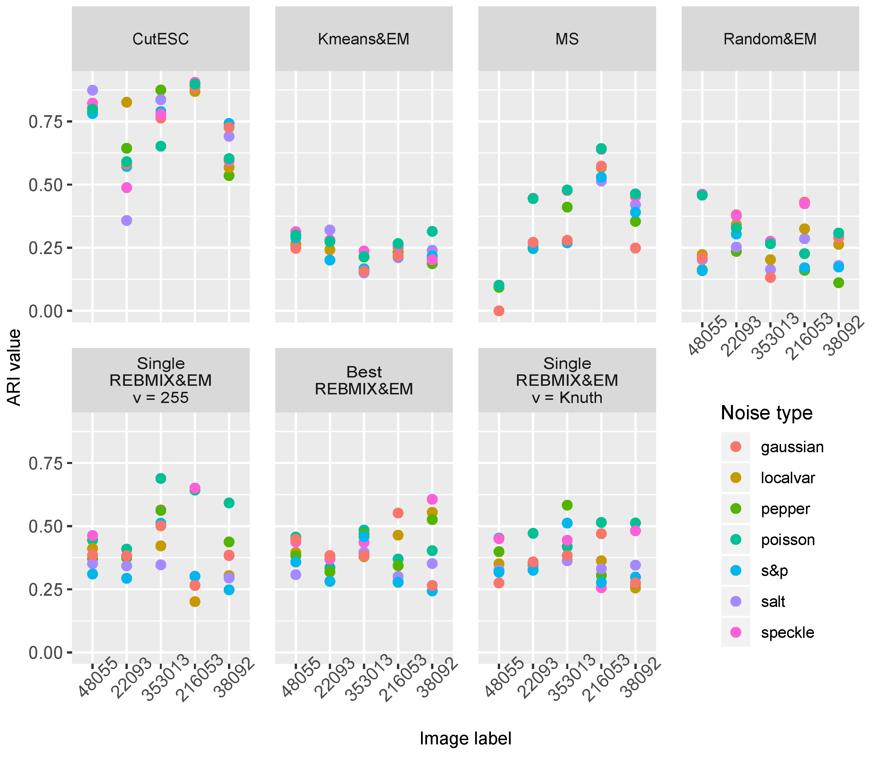
CutESC	0.86	0.71	0.92	0.79	0.76

summarizes the ARI values obtained using their algorithms. In addition, to obtain consistently good segmentations for the CutESC algorithm, parameters $\alpha$ and $\beta$ were set to 0.5. As expected, CutESC outperformed all the other strategies/algorithm. The GMM estimated with the REBMIX&EM strategies outperformed the MS clustering algorithm on images 353013, 38092 and 48055, and MS yielded slightly better results on images 216053 and 22093.

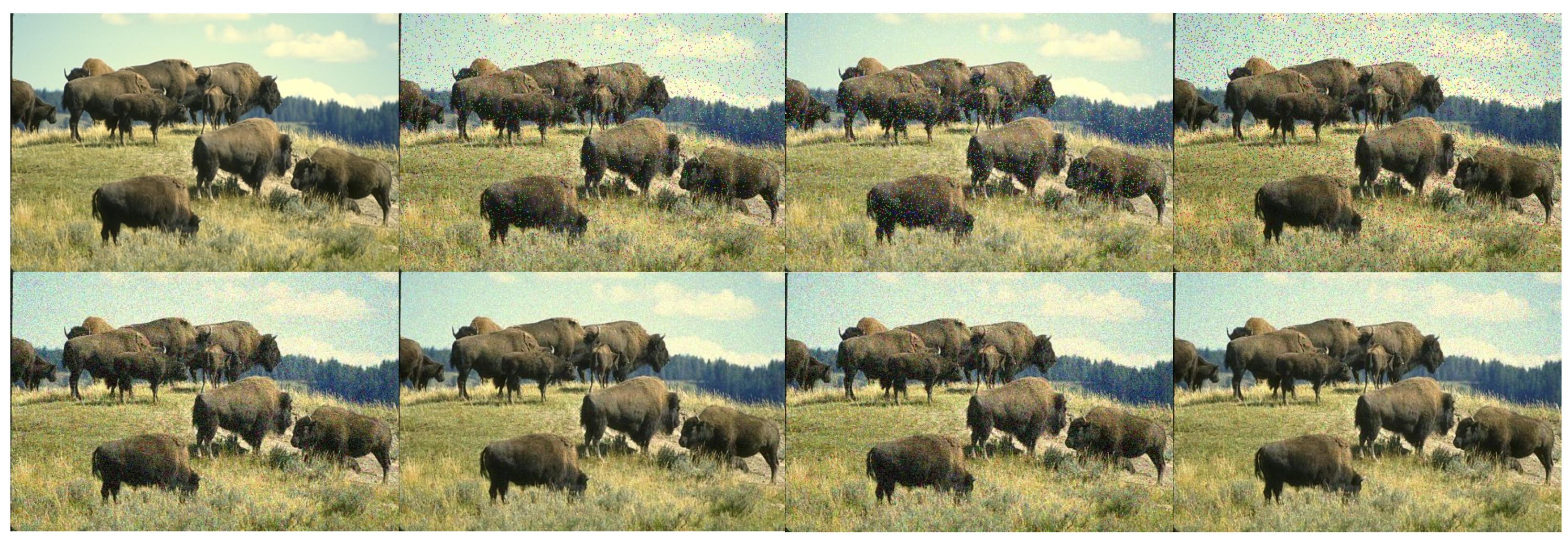
To investigate the robustness of the different strategies in a clustering scenario of the image-segmentation tasks, we added different types of noise to the images used. Seven types of noise, salt, pepper, salt&pepper or shortly (s&p), Gaussian, Poisson, speckle, localvar implemented in the Scikit-image python module, and their effects can be seen in the herd image in Figure 10. The results of the ARI value are shown on the plots in Figure 11 for each strategy/method and the corresponding image and noise type.

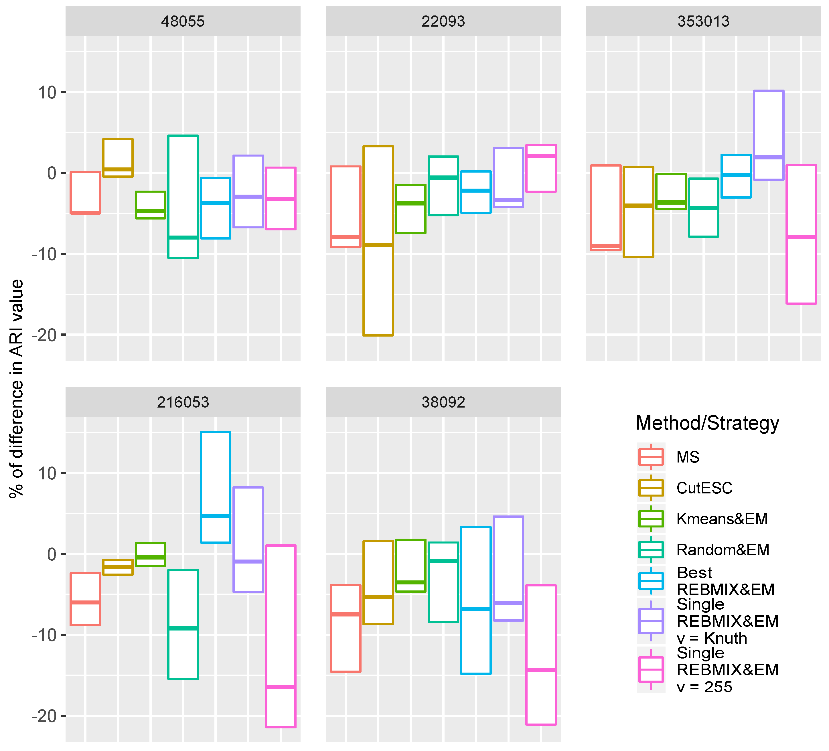
As expected, the different types of noise contributed differently to the quality of the segmentation; however, surprisingly, not all the types of noise deteriorated the results in terms of reducing the ARI value. The Poisson had an improving effect on almost every image and every method/strategy used. Noises such as salt, pepper and salt&pepper generally had a deteriorating effect on the results of the segmentation. With certain methods/strategies, this type of noise deteriorated the quality of the segmentation by up to 20%. In order to better evaluate the results, we provided additional box-plots (Figure 12) of the different methods/strategies that show the percentage of difference between the results of the non-noisy images and the results of the noisy images. The box-plots are constructed as follows. The upper limit of the box is the maximum value of the difference (positive value means improvement), and the lower limit is the minimum value (negative value means deterioration) and the horizontal line within the box median value. Since the ARI measure is bounded between −1 and 1, the difference of 10% can be interpreted as 0.05 of the difference of the ARI value.

The following general remarks can be derived from the box plots in Figure 12. The results of the segmentation from the MS algorithm have usually deteriorated. However, this deterioration was only minor and ranged from 5% up to 10%. On the other hand, the CutESC algorithm on the image 48055 mostly had improvements, while on the image 216053 it produced only a slight deterioration of the segmentation results. On the image 22093, there were slight improvements in the segmentation results for certain noise types, while there were large deteriorations for the others. On the images 353013 and 38092, the noise usually deteriorated the segmentation results from the CutESC algorithm. Forwardly, the noise had the following effects on the results of the segmentation using the Kmeans&EM and Random&EM strategies. Different noise types had little effect (either improving or deteriorating) on the segmentation results with the Kmeans&EM strategy, while the noise deteriorated the segmentation results with the Random&EM strategy in most cases, although the specific noise types improved the segmentation results for the images 48055 and 22093.

The REBMIX&EM strategies used were influenced by the noise and the different types of noise in different ways. We will start with the Single REBMIX&EM strategy with the number of bins $v=255$. This strategy had the greatest deterioration for the images 353013, 216053, and 38092. Although it is still not as significant, since 20% represents the decrease of the ARI value of 0.1, it indicates that this method should be used with caution in the presence of noise. On the other hand, the Best REBMIX&EM and Single REBMIX&EM strategy with the number of bins v estimated with the Knuth rule had minor to mild (image 38092 with Best REBMIX&EM strategy) deterioration of the segmentation results, and, interestingly, the greatest improvements of the segmentation results in the presence of different types of noise. In fact, the Best REBMIX&EM only had improvements of the segmentation results for the image 216053 without any deterioration (the resulting rectangle in Figure 12 is above zero). The Single REBMIX&EM strategy with the number of bins v estimated with the Knuth rule had similar results for the 353013 image. This can be interpreted as follows. By adding noise to particular images, the density shape of the image pixel values became more similar to those that the GMM can generate, so the REBMIX&EM strategies were able to successfully estimate them.

The results of the different strategies/algorithms regarding image segmentation with noise applied to the images revealed some interesting facts, such as the fact that adding some types of noise could improve the results of the GMM-based image segmentation. The in-depth investigation of when and why this happened goes beyond the scope of this article and also goes beyond the topic, so we conclude with a final remark. In many cases, the noise will deteriorate the results of the segmentation; however, this is to be expected. For most of the strategies/algorithms used, the amount of deterioration was low. If the present amount of noise is large, the Random&EM strategy or the Single REBMIX&EM with the number of bins $v=255$ is not recommended, while the others are safe to use. It should also be considered as to whether the addition of some artificial noise can improve the result of the segmentation.

5.4. Comparison of the Time Complexity of REBMIX and k-Means Algorithm

As the k-means algorithm is more or less the fastest used algorithm to initialize the parameters for the EM estimation of the GMM, we compared the time complexity of the k-means algorithm and the REBMIX algorithm. It is hard to estimate theoretically the time complexity for both algorithms. Judging by [31], the theoretical time complexity of the k-means is $O\left(tcnd\right)$, where t is the number of iterations needed, c is the number of components, n is the number of observations, and d is the dimension of the dataset. It is hard to know how many iterations t will the k-means algorithm need. On the other hand, the time complexity of the REBMIX algorithm depends on multiple factors. First, the most important is definitely the number of non-empty bins $v^{*}$ in the histogram preprocessing. Forward, it depends on the chosen maximum value of the components $c_{\max }$ and the dimension of the problem d. 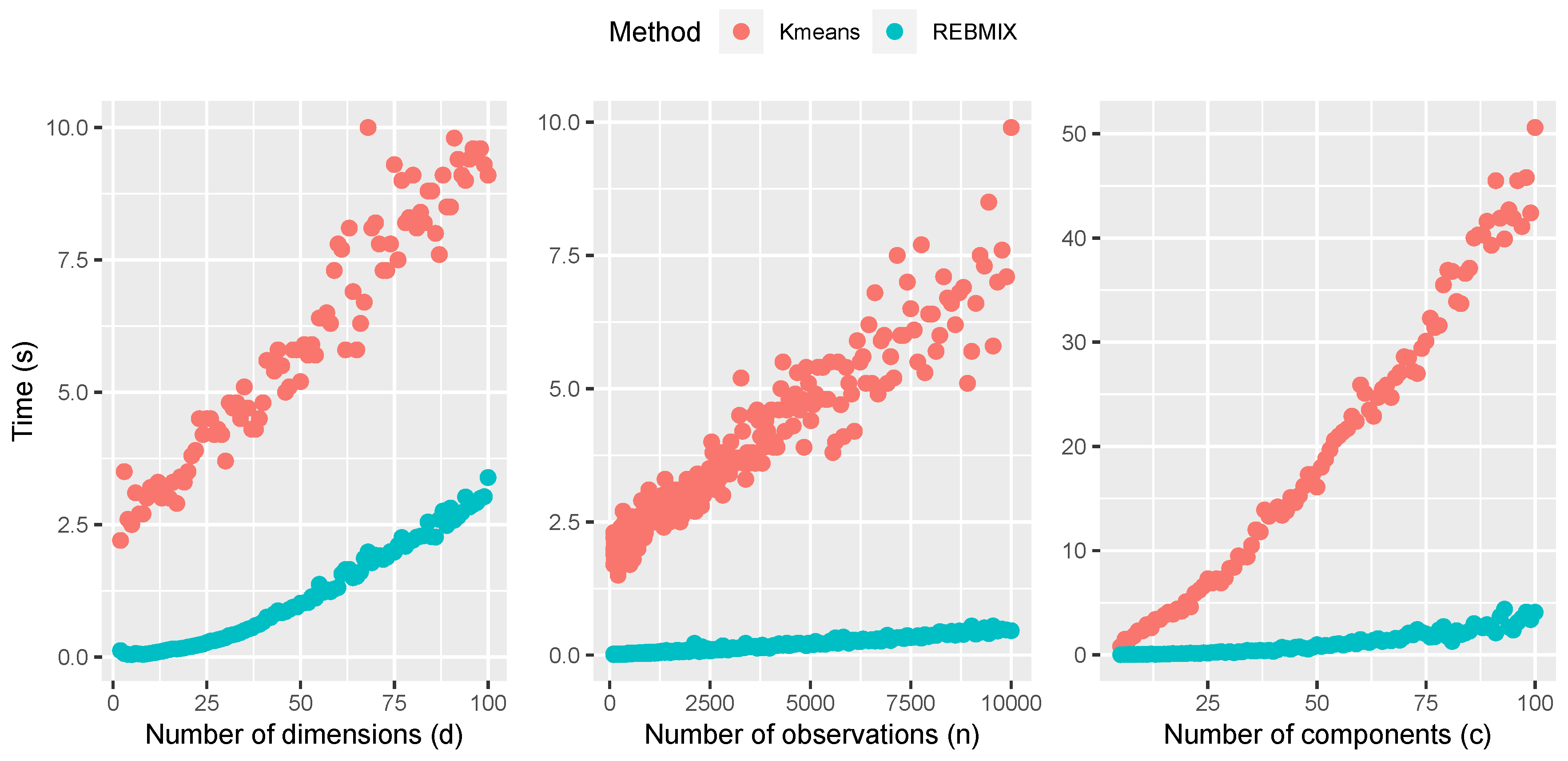Finally, it depends on the different number of bins v for the histogram preprocessing, e.g., the 3–100 range has 97 values. Therefore, we have chosen to give an empirical comparison of both algorithms in terms of the number of observations n, the number of dimensions d, and the maximum number of components $c_{\max }$. The results are presented in Figure 13. For the REBMIX algorithm, we used the REBMIX function provided by the rebmix R package. For the k-means algorithm, we used the default R kmeans implementation provided in the base R package. Although the k-means algorithm needs a different number of iterations, here we considered 100 iterations of the k-means algorithm. This seems reasonable due to the fact that repetitions of the k-means are often preferable [31]. In addition, due to the fact that, for the GMM initialization, the k-means algorithm needs to be repeated $c_{\max }-c_{\min }$ times, we have taken this into consideration by repeating the k-means algorithm for each $c\in \{c_{\min },c_{\min }+1,\cdots ,c_{\max }\}$. For the REBMIX algorithm, we have used the setting in which the number of bins v is not known and the range used was 3–100. In addition, when the time complexity with respect to the one parameter is evaluated, the other two were kept constant. In other words, when comparing the time complexity with respect to the number of dimensions d, the number of observations $n=1000$ and the maximum number of components $c_{\max }=10$ was kept constant. For the comparison with respect to the number of observations n, the number of dimensions was $d=5$ and the maximum number of components $c_{\max }=10$. Finally, for the comparison with respect to the maximum number of components $c_{\max }$, the number of dimensions was $d=5$ and the number of observations was $n=1000$.

First, we will start with a comparison with respect to the number of dimensions d, which is given in the first plot of Figure 13. We can see that the time complexity of k-means is linear with respect to this parameter. Therefore, it agrees with the theoretical assumption. On other hand, the REBMIX seems to have a nonlinear complexity with respect to the parameter d. The nonlinearity with respect to this parameter comes from the definition of the multivariate Gaussian distribution in Equation (2). To calculate the PDF of the GMM, the inverse of the covariance matrix $\mathit{\Sigma }$ for each component is required. The matrix inversion is a nonlinear operation; therefore, nonlinear dependence in time is justified. The second parameter for which the comparison was made was the number of observations n in the dataset. The results are shown on second plot of Figure 13. Both the REBMIX and k-means algorithms exhibited a linear dependency in respect to the number of observations n, and, finally, k-means had a linear dependency with respect to the $c_{\max }$ parameter, while the REBMIX has nonlinear. The nonlinear complexity in terms of the parameter $c_{\max }$ comes from its empirical stopping criteria, which does not guarantee that each iteration adds exactly one more component to the GMM (details of the stopping criteria of the REBMIX algorithm are explained in the last two paragraphs of Section 3.2). The nonlinear dependencies of the REBMIX algorithm with respect to the parameters d and $c_{\max }$ are troublesome, given that k-means has a linear dependence. This gives the k-means algorithm an advantage over the REBMIX algorithm. However, if the time complexity with respect to the number of observations n is observed, they have proven to be equal competitors. In the end, with the obtained values of time spent for the REBMIX algorithm and the k-means algorithm, the REBMIX algorithm was generally faster.

5.5. Note on Selection of Hyperparameters for the REBMIX&EM Strategies and Their Impact on Performance

In this section, we will discuss the hyperparameters of the REBMIX&EM strategies used for the presented experiments. There were five different hyperparameters used for all the experiments, in particular the number of bins v, the minimum number of components $c_{\min }$ in the GMM, the maximum number of components $c_{\max }$ in the GMM, the maximum number of iterations of the EM algorithm, and the threshold for convergence of the EM algorithm.

First, we will discuss the choice of the number of bins v for the histogram preprocessing. There is no general rule for estimating the number of bins v in the histogram [44]. Some common estimators are Sturges’ rule ${log}_2\left(n\right)+1$ originating in [45] and the RootN rule $\sqrt{n}$ from [46]. In [16], it was suggested to create the lower and upper bounds for the bin range K based on these rules. Strurges’ rule always yields a smaller number of bins v and is suitable for the lower bound, while the RootN rule gives a larger number of bins v and thus can be used for the upper bound. The ranges K based on those two rules are narrow for datasets with a smaller number of observations n, e.g., for $n=100$, the range is 7–10 bins. For the dataset with a large number of observations, e.g., n = 10,000 leads to the range of 14–100, which is very wide. The choice of the bin range 3–100 as a constant for each experiment was chosen to test whether these additional ranges can be used to better estimate the GMM parameters using the REBMIX algorithm and thus allow a better initialization of the EM algorithm, or only cause an unnecessary computational effort. 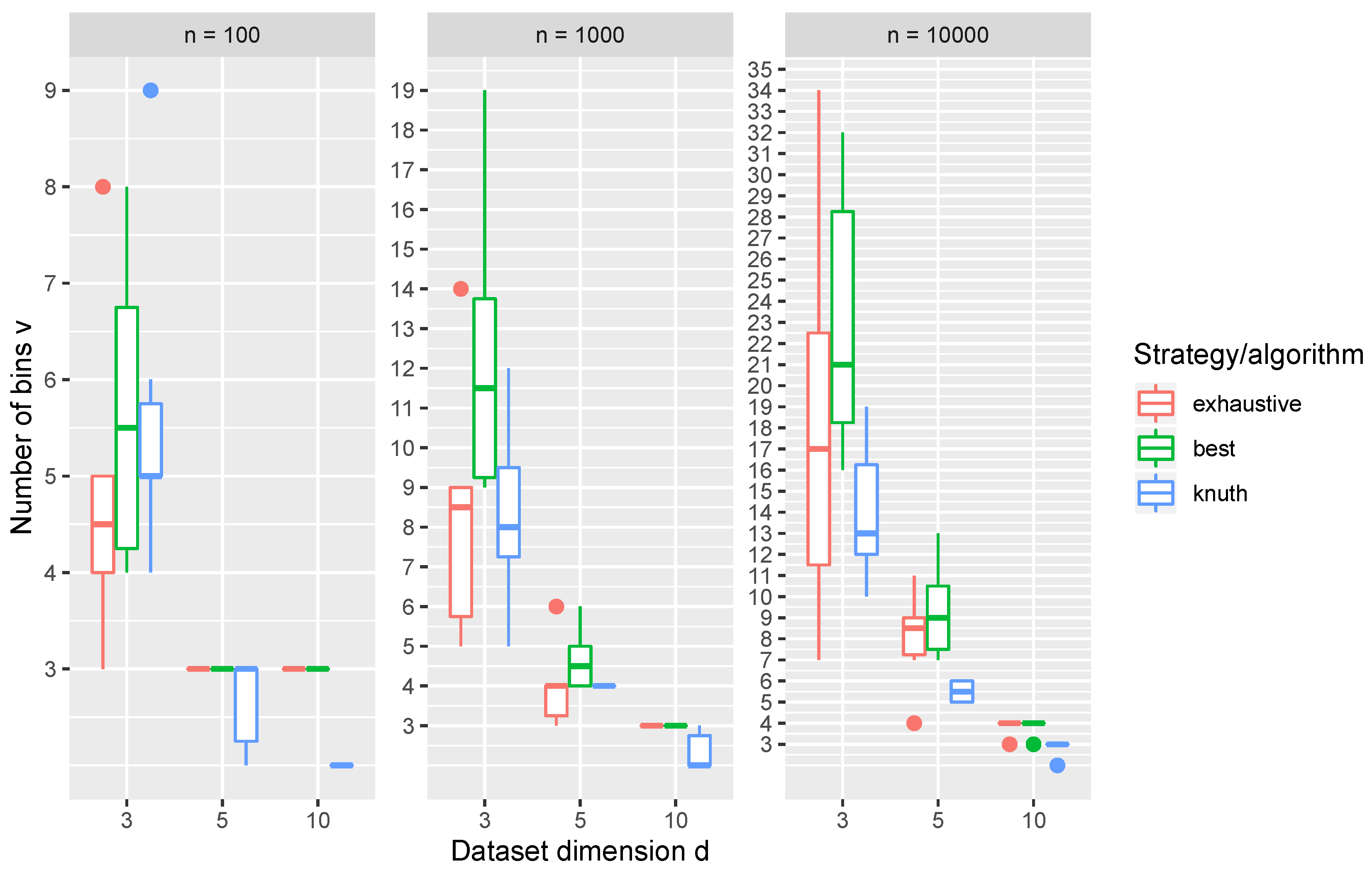For the estimation of the number of bins v for the Single REBMIX&EM strategy, we have used the Knuth rule. The Knuth rule uses a Bayesian approach to estimate the number of bins v in a histogram, thus making this estimation dependent on the observations from the dataset. Ref. [40] gives a straightforward extension to multivariate histograms. Although, in the original paper, the multivariate histograms can have a different number of bins for each dimension, i.e., $v_i,\forall i\in \{1,2,\cdots ,d\}$, it is worth noting that we only used the same number of bins v in each dimension. The number of bins v estimated with the Knuth rule for datasets from Section 4.1 is shown in Figure 14. It is clear from Figure 14 that the Knuth rule depends on both the dimension d of the dataset and the number of observations n, unlike the above-mentioned estimators. In addition, it had a different number of bins v for the datasets with the same dimension d and number of observations n (boxes span over multiple values of v), which indicates that n and d are not the only influences. In addition, it is clear that the number of bins v is greatly reduced as the dimensions of the dataset increased. This can be tied to what is called the curse of dimensionality [44]. There are many bins in a high-dimensional histogram grid. Just for the $v=3$ and $d=10$ settings, there are 9,765,625 bins. Such an extremely large number of bins leads to many empty bins, i.e., for which the frequency was $k_j=0$, which were heavily penalized by the Knuth rule (it can be seen that, for $d=10$, the estimated number of bins was mostly $v=2$ or $v=3$).

Additionally, in Figure 14, the number of bins v that yielded the optimal GMM parameters using the Exhaustive and Best REBMIX&EM strategies given for the datasets. Although we have given a large range, judging by the values in Figure 14, it can be seen that both the Exhaustive and the Best REBMIX&EM strategies estimated the GMM parameters for a different number of bins v than what is proposed by the Knuth estimator, which leads in some experiments to benefits, while in another leads to some numerical instabilities. For example, the number of optimal GMM parameters estimated with the Exhaustive REBMIX&EM strategy was the greatest if we recall Figure 4. On the other hand, regarding what was found by comparing the density-estimation performance in Section 5.1.2 for a small number of observations $n=100$, this caused some of the degeneracies in the estimated GMM parameters. The Best REBMIX&EM strategy favored a larger number of bins v in the histogram preprocessing in all the presented cases. This is also a useful insight because in the image-segmentation experiment (Table 3) the results were better than what was acquired with a Single REBMIX&EM strategy with the number of bins v estimated with the Knuth rule. For the density-estimation tasks in Section 5.2, the results seem to have not been very impacted by the chosen REBMIX&EM strategy, at least in terms of the MISE value (Figure 7). Let us recall that we also used the intuitive $v=255$ for the image-segmentation tasks. As we already said, this intuition was made based on the fact that digital images have 255 different intensity values for each color channel. This assumption was shown to be good, judging by the results we obtained with it; however, it was probably most sensitive to the noise along with the Random&EM strategy.

To conclude, the Single REBMIX&EM strategy with the Knuth rule can be safely used when a short computation time is preferred, and the dimension of the dataset is small. The datasets in the density-estimation tasks in Section 5.2 had $d=2$ or $d=3$. For the Exhaustive and Best REBMIX&EM strategies, we recommend the RootN rule for the upper bound and the Knuth rule for the lower bound. The RootN rule will mostly overestimate the number of bins for larger n, judging by the obtained values in Figure 14. However, due to the fact that a smaller number of EM iterations was needed with the REBMIX, as an initialization technique, this remains acceptable. If the time efficacy is a major concern, to obtain the best-possible results for the datasets with a larger number of observations n, the Best REBMIX&EM strategy could be used to obtain the upper bound for the histogram preprocessing number of bins v range. Then, the Exhaustive REBMIX&EM strategy could be used with this value as the upper bound, while keeping the Knuth rule for the lower bound, for the histogram preprocessing number of bins v range.

We would like to mention some points about the selection of the $c_{\min }$ and $c_{\max }$ values for the GMM or any other MM parameter estimation. The number of MM parameters increases with the increasing dimension, especially the GMM parameters. It is, therefore, always advisable to check to see whether the number of observations n in the dataset is larger than the number of parameters M, i.e., $n\ge M$. For a dataset with a smaller number of observations n, this can be used as a rule-of-thumb selector of $c_{\max }$. Choosing a smaller value for $c_{\max }$ when the number of observations n is also small can additionally reduce the probability of estimating the degenerated solution. Otherwise, the maximum number of components $c_{\max }$ can be as large as required, depending on the application of the GMM. For example, in the image-segmentation tasks, the number of observations was large. As can be seen in Table 3, the estimated number of components c was always high. The images used had a resolution of 480 × 320 or 320 × 480, which resulted in a number of observations equal to n =153,600. Based on our above rule of thumb, the value of $c_{\max }$ can go as high as $c_{\max }$ = 15,000. However, this would be numerically unstable due to the floating arithmetic. For this kind of example, where the number of observations n is high and we can expect a large number of components in the GMM, this hyperparameter can also be fine-tuned. Some lower value can be used as the starting point to obtain some information about how the IC (in our case the BIC) is changing with respect to an increase in the number of components c in the GMM. If there are some large fluctuations in the value of BIC, or the slope of the BIC-c curve seems too steep, we can try to increase the value of $c_{\max }$ until the curve stabilizes and the values of BIC slowly start to increase. If some other IC is used instead of the BIC, then the same analogy applies. As for the $c_{\min }$, it is advisable to use $c_{\min }=1$ for the minimum value to check whether the dataset fits well into the non-mixture distribution.

For the values of the maximum number of iterations of the EM algorithm and the threshold of the EM algorithm, we have chosen 1000 and 0.0001, respectively. These two values are chosen in this paper based on some empirical evidence from other software that implemented the EM algorithm (for example, Sklearn’s EM implementation for the GMM estimation has a default value of 100 maximum iterations and 0.001 for the average log-likelihood threshold). Choosing these values should always be based on pragmatic grounds, i.e., we expect that this threshold can be reached in this amount of iterations. For example, the authors of [25] argue that even perhaps the most efficient way of managing the convergence of the EM algorithm, for the GMM parameter estimation, is to use only the specified number of iterations as stopping criteria because setting small threshold values can be hazardous in terms of the computation times due to the unboundedness of the log-likelihood function. However, in our experiments, we have observed that the REBMIX algorithm tends to estimate the initial parameters close to the final ones and we usually did not even use half of the expected iterations (see the second plot in Figure 4). To conclude, we can safely recommend these values as starting points; however, if necessary, fine-tuning can also be applied.

6. Conclusions

We have proposed the use of the REBMIX algorithm as an initialization technique for the EM algorithm, as applied to the MM parameter-estimation problem. Additionally, three different strategies are proposed when the number of components in the MM is unknown. The proposed strategies were thoroughly tested on artificially created datasets (Section 5.1), density-estimation tasks (Section 5.2), and image-segmentation tasks (Section 5.3). Our proposals showed benefits in terms of accuracy as well as with the computational efficacy. While preserving good or even better results from various applications of the GMM, fewer of the more expensive EM iterations were needed for the EM to converge. Moving forward, the proposed initialization and strategies when applied to real-world tasks, such as density estimation and image segmentation, were again competitive and even better with the state-of-the-art initialization strategies and, additionally, with the state-of-the-art algorithms for density estimation and image-segmentation (clustering), respectively. Moreover, the proposed initialization and strategies provided comparable or better results compared to the ADEBA algorithm in terms of computational effectiveness, as was shown in Figure 8. In addition, we provided some insights into the time complexity of the REBMIX algorithm in Section 5.4. Even though we did not provide a theoretical proof of the time complexity, which was due to multiple stochastic factors impacting on its performance, from the empirical evaluation, it can be seen that REBMIX has linear time with respect to the parameter n and a nonlinear time with respect to the parameters c and d. On other hand, the k-means algorithm was linear with respect to all three parameters. However, the actual value of the computation times in Figure 13 showed that REBMIX was faster than k-means for this specific case. On the third plot in Figure 4 and Figure 8, we have provided some empirical insights into the time efficacy of the proposed REBMIX&EM strategies. Here, the theoretical estimation of the time complexity classes, due to the use of the EM algorithm, which does not have clear termination criteria, was not provided. That being said, we have given our best effort to provide enough critical empirical insights with which we can state that our proposal is more time efficient with regard to the state-of-the-art approaches.

From the paragraph above, the main advantages of our proposal with regard to the state of the art can be extracted. Our proposal was time efficient and had good results. The current state-of-the-art approach, nevertheless, of the initialization technique used, is to try the EM algorithm on as many initializations as possible in a selected/given amount of time. Therefore, algorithms/initialization that can provide multiple repeats are preferred. The REBMIX heuristic is deterministic and cannot be improved with multiple restarts. We see this as the main disadvantage with regard to the state-of-the-art approaches. For a given number of bins v, it will always estimate the same parameters of the GMM. In addition, this parameter, i.e., the number of bins v, is usually not known in advance. Therefore, we proposed the use of the Exhaustive and Best REBMIX&EM strategies. Both strategies are more computational demanding when compared to the Single REBMIX&EM strategy. Furthermore, the choices we made for the number of bins v are thoroughly described in Section 5.5. We see this task of choosing the appropriate range of the number of bins, or some specific value or set of specific values, as the largest overhead introduced with our proposal. Other state-of-the-art strategies do not need this kind of parameter, only the rest of the hyperparameters ($c_{\max }$, $c_{\min }$, maximum number of iterations, and threshold). Some smaller limitations were also encountered. Namely, datasets with a large dimension d and small number of observations n led to some degeneracies in the estimates. Therefore, at this point, our proposal cannot be recommended for such problems. We did not include any safeguards for the EM algorithm and thus this happened. The empirically evaluated time complexity of the REBMIX algorithm showed some problems. The nonlinearity in terms of the dimension of the dataset d was to be expected, while the nonlinearity in terms of the maximum number of components $c_{\max }$ was troublesome. This overhead introduced with our proposal can be burdensome, especially with larger values of the parameter $c_{\max }$.

To conclude this article, let us say that we have implemented all our proposals in the rebmix R package (https://cran.r-project.org/web/packages/rebmix/index.html), and they are ready to use. In addition, let us explain how our work can be extended. First, the Bayesian regularization for the EM algorithm could be used to additionally avoid degeneracies and constrict the likelihood [14]. Second, the use of the GMM for certain image-segmentation tasks and the density-estimation tasks was questionable, like for the flower image or the Bend distribution. Although we have used the GMM as a proof of concept, our work can be extended to other types of MMs. For the extension to the other parametric family of the MM, the equations for the REBMIX and EM algorithms need to be derived. In [17], it was shown how the REBMIX algorithm can be extended to other types of MM, particularly to the von-Mises MM. For the EM algorithm, the M-step equations need to be derived. For example, in [18], the derivation of the Weibull-Normal MM parameters is given. In addition, there is a plethora of literature about how the EM can be extended to other parametric families [9,10] to name just a few. We will strive to provide some more theoretical insights into the REBMIX algorithm. Specifically, the empirical equation for decreasing the parameter $D_{\min }$ should be improved to avoid nonlinear time complexity in terms of the parameter $c_{\max }$. The hyperparameter, the number of bins v for the histogram preprocessing, needs special care. For the histogram preprocessing, we only used the same number of bins in each dimension, although the number of bins can be different in each dimension, or, finally, some adaptive bandwidth for the histogram preprocessing can be applied, like the ones used for a kernel density estimation in [11]. Some other REBMIX preprocessing capabilities like kernel density or k-nearest neighbor could be used. In the end, the application of the MM for the image segmentation should be more thoroughly researched. Throughout the testing of the proposals for the image-segmentation tasks, we encountered some interesting facts outlined in Section 5.3. As this was not the primary problem of this article, we left this topic open to be revisited.

References

1. Dempster, A.P.; Laird, N.M.; Rubin, D.B. Maximum likelihood from Incomplete Data via the EM Algorithm. J. R. Stat. Soc. 1977, 39, 1–38. [Google Scholar]
2. Yu, J.; Chaomurilige, C.; Yang, M.S. On convergence and parameter selection of the EM and DA-EM algorithms for Gaussian mixtures. Pattern Recognit. 2018, 77, 188–203. [Google Scholar] [CrossRef]
3. Ma, J.; Jiang, X.; Jiang, J.; Gao, Y. Feature-guided Gaussian mixture model for image matching. Pattern Recognit. 2019, 92, 231–245. [Google Scholar] [CrossRef]
4. Liu, C.; Li, H.C.; Fu, K.; Zhang, F.; Datcu, M.; Emery, W.J. Bayesian estimation of generalized Gamma mixture model based on variational EM algorithm. Pattern Recognit. 2019, 87, 269–284. [Google Scholar] [CrossRef]
5. Du, Y.; Gui, W. Goodness of Fit Tests for the Log-Logistic Distribution Based on Cumulative Entropy under Progressive Type II Censoring. Mathematics 2019, 7, 361. [Google Scholar] [CrossRef] [Green Version]
6. Pagès-Zamora, A.; Cabrera-Bean, M.; Díaz-Vilor, C. Unsupervised online clustering and detection algorithms using crowdsourced data for malaria diagnosis. Pattern Recognit. 2019, 86, 209–223. [Google Scholar] [CrossRef] [Green Version]
7. Yu, L.; Yang, T.; Chan, A.B. Density-Preserving Hierarchical EM Algorithm: Simplifying Gaussian Mixture Models for Approximate Inference. IEEE Trans. Pattern Anal. Mach. Intell 2019, 41, 1323–1337. [Google Scholar] [CrossRef] [PubMed]
8. Gebru, I.D.; Alameda-Pineda, X.; Forbes, F.; Horaud, R. EM Algorithms for Weighted-Data Clustering with Application to Audio-Visual Scene Analysis. IEEE Trans. Pattern Anal. Mach. Intell 2016, 38, 2402–2415. [Google Scholar] [CrossRef] [PubMed] [Green Version]
9. McLachlan, G.; Peel, D. Finite Mixture Models, 1st ed.; John Wiley & Sons: Hoboken, NJ, USA, 2000. [Google Scholar]
10. McLachlan, G.; Krishnan, T. The EM Algorithm and Extensions, 2nd ed.; John Wiley & Sons: Hoboken, NJ, USA, 2007. [Google Scholar]
11. Bäcklin, C.L.; Andersson, C.; Gustafsson, M.G. Self-tuning density estimation based on Bayesian averaging of adaptive kernel density estimations yields state-of-the-art performance. Pattern Recognit. 2018, 78, 133–143. [Google Scholar] [CrossRef]
12. Yang, M.S.; Lai, C.Y.; Lin, C.Y. A robust EM clustering algorithm for Gaussian mixture models. Pattern Recognit. 2012, 45, 3950–3961. [Google Scholar] [CrossRef]
13. Celeux, G.; Govaert, G. Gaussian parsimonious clustering models. Pattern Recognit. 1995, 28, 781–793. [Google Scholar] [CrossRef] [Green Version]
14. Baudry, J.P.; Celeux, G. EM for mixtures. Stat. Comput. 2015, 25, 713–726. [Google Scholar] [CrossRef]
15. Ng, S.K.; McLachlan, G.J. Speeding up the EM algorithm for mixture model-based segmentation of magnetic resonance images. Pattern Recognit. 2004, 37, 1573–1589. [Google Scholar] [CrossRef]
16. Nagode, M. Finite Mixture Modeling via REBMIX. J. Algorithms Optim. 2015, 3, 14–28. [Google Scholar] [CrossRef]
17. Ye, X.; Xi, P.; Nagode, M. Extension of REBMIX algorithm to von Mises parametric family for modeling joint distribution of wind speed and direction. Eng. Struct. 2019, 183, 1134–1145. [Google Scholar] [CrossRef]
18. Franko, M.; Nagode, M. Probability density function of the equivalent stress amplitude using statistical transformation. Reliab. Eng. Syst. Saf. 2015, 134, 118–125. [Google Scholar] [CrossRef]
19. Gallaugher, M.P.; McNicholas, P.D. Finite mixtures of skewed matrix variate distributions. Pattern Recognit. 2018, 80, 83–93. [Google Scholar] [CrossRef] [Green Version]
20. Franczak, B.C.; Browne, R.P.; McNicholas, P.D. Mixtures of Shifted Asymmetric Laplace Distributions. IEEE Trans. Pattern Anal. Mach. Intell 2014, 36, 1149–1157. [Google Scholar] [CrossRef] [Green Version]
21. Wang, H.; Luo, B.; Zhang, Q.; Wei, S. Estimation for the number of components in a mixture model using stepwise split-and-merge EM algorithm. Pattern Recognit. Lett. 2004, 25, 1799–1809. [Google Scholar] [CrossRef]
22. Zhang, B.; Zhang, C.; Yi, X. Competitive EM algorithm for finite mixture models. Pattern Recognit. 2004, 37, 131–144. [Google Scholar] [CrossRef]
23. Figueiredo, M.A.T.; Jain, A.K. Unsupervised learning of finite mixture models. IEEE Trans. Pattern Anal. Mach. Intell 2002, 24, 381–396. [Google Scholar] [CrossRef] [Green Version]
24. Ari, Ç.; Aksoy, S.; Arıkan, O. Maximum likelihood estimation of Gaussian mixture models using stochastic search. Pattern Recognit. 2012, 45, 2804–2816. [Google Scholar] [CrossRef]
25. Biernacki, C.; Celeux, G.; Govaert, G. Choosing starting values for the EM algorithm for getting the highest likelihood in multivariate Gaussian mixture models. Comput. Stat. Data Anal. 2003, 41, 561–575. [Google Scholar] [CrossRef]
26. Melnykov, V.; Melnykov, I. Initializing the EM algorithm in Gaussian mixture models with an unknown number of components. Comput. Stat. Data Anal. 2012, 56, 1381–1395. [Google Scholar] [CrossRef]
27. Michael, S.; Melnykov, V. An effective strategy for initializing the EM algorithm in finite mixture models. Adv. Data Anal. Classif. 2016, 10, 563–583. [Google Scholar] [CrossRef]
28. Kwedlo, W. A new random approach for initialization of the multiple restart EM algorithm for Gaussian model-based clustering. Pattern Anal. Appl. 2015, 18, 757–770. [Google Scholar] [CrossRef] [Green Version]
29. Maitra, R. Initializing Partition-Optimization Algorithms. IEEE/ACM Trans. Comput. Biol. Bioinform. 2009, 6, 144–157. [Google Scholar] [CrossRef]
30. Zhao, Q.; Hautamäki, V.; Kärkkäinen, I.; Fränti, P. Random swap EM algorithm for Gaussian mixture models. Pattern Recognit. Lett. 2012, 33, 2120–2126. [Google Scholar] [CrossRef]
31. Fränti, P.; Sieranoja, S. How much can k-means be improved by using better initialization and repeats? Pattern Recognit. 2019, 93, 95–112. [Google Scholar] [CrossRef]
32. Scrucca, L.; Raftery, A.E. Improved initialisation of model-based clustering using Gaussian hierarchical partitions. Adv. Data. Anal. Classif. 2015, 9, 447–460. [Google Scholar] [CrossRef] [Green Version]
33. Bishop, C. Pattern Recognition and Machine Learning; Springer: Berlin/Heidelberg, Germany, 2006. [Google Scholar]
34. Nagode, M.; Fajdiga, M. The REBMIX Algorithm for the Univariate Finite Mixture Estimation. Commun. Stat. Theory Methods 2011, 40, 876–892. [Google Scholar] [CrossRef]
35. Nagode, M.; Fajdiga, M. The REBMIX Algorithm for the Multivariate Finite Mixture Estimation. Commun. Stat. Theory Methods 2011, 40, 2022–2034. [Google Scholar] [CrossRef]
36. Nagode, M. Multivariate normal mixture modeling, clustering and classification with the rebmix package. arXiv 2018, arXiv:stat.ML/1801.08788. [Google Scholar]
37. Melnykov, V.; Chen, W.C.; Maitra, R. MixSim: An R Package for Simulating Data to Study Performance of Clustering Algorithms. J. Stat. Softw. 2012, 51, 1–25. [Google Scholar] [CrossRef] [Green Version]
38. Hubert, L.; Arabie, P. Comparing partitions. J. Classif. 1985, 2, 193–218. [Google Scholar] [CrossRef]
39. Martin, D.; Fowlkes, C.; Tal, D.; Malik, J. A Database of Human Segmented Natural Images and its Application to Evaluating Segmentation Algorithms and Measuring Ecological Statistics. In Proceedings of the Eighth IEEE International Conference on Computer Vision, Vancouver, BC, Canada, 7–14 July 2001; Volume 2, pp. 416–423. [Google Scholar]
40. Knuth, K.H. Optimal Data-Based Binning for Histograms. arXiv 2006, arXiv:physics/0605197. [Google Scholar]
41. Aksac, A.; Özyer, T.; Alhajj, R. CutESC: Cutting edge spatial clustering technique based on proximity graphs. Pattern Recognit. 2019, 96, 106948. [Google Scholar] [CrossRef]
42. Pedregosa, F.; Varoquaux, G.; Gramfort, A.; Michel, V.; Thirion, B.; Grisel, O.; Blondel, M.; Prettenhofer, P.; Weiss, R.; Dubourg, V.; et al. Scikit-learn: Machine Learning in Python. J. Mach. Learn. Res. 2011, 12, 2825–2830. [Google Scholar]
43. Van der Walt, S.; Schönberger, J.L.; Nunez-Iglesias, J.; Boulogne, F.; Warner, J.D.; Yager, N.; Gouillart, E.; Yu, T. scikit-image: Image processing in Python. PeerJ 2014, 2, e453. [Google Scholar] [CrossRef]
44. Scott, D.W.; Sain, S.R. 9—Multidimensional Density Estimation. In Data Mining and Data Visualization; Rao, C., Wegman, E., Solka, J., Eds.; Handbook of Statistics; Elsevier: Amsterdam, The Netherlands, 2005; Volume 24, pp. 229–261. [Google Scholar]
45. Sturges, H.A. The Choice of a Class Interval. J. Am. Stat. Assoc. 1926, 21, 65–66. [Google Scholar] [CrossRef]
46. Velleman, P.F. Interactive Computing for Exploratory Data Analysis I: Display Algorithms. In Proceedings of the Statistical Computing Section; American Statistical Association: Washington, DC, USA, 1976. [Google Scholar]
Figure 1. Illustration of the REBMIX algorithm on Old Faithful geyser data.
Mathematics 08 00373 g001
Figure 2. Examples of artificial datasets with two dimensions and five components with a variable number of observations and an overlap level. The upper three graphs had a = 0 . 001 and the lower three graphs had a = 0 . 125 . From left to right, the number of observations were respectively n = 100 , n = 1000 , and n = 10,000.
Mathematics 08 00373 g002
Figure 3. Showcase of selected images from [39]. First row: flower image (label 353013; herd image (label 38092); woman image (label 216053). Second row: fisherman image (label 48055); bridge image (label 22093).
Mathematics 08 00373 g003
Figure 4. Benchmarking different REBMIX&EM strategies vs. Kmeans&EM and Random&EM.
Mathematics 08 00373 g004
Figure 5. Clustering performance of the Exhaustive REBMIX&EM strategy, Best REBMIX&EM strategy, Single REBMIX&EM strategy, Kmeans&EM, Random&EM, and REBMIX on artificial datasets.
Mathematics 08 00373 g005
Figure 6. Density-estimation performance evaluation of Exhaustive REBMIX&EM strategy, Best REBMIX&EM strategy, Single REBMIX&EM strategy, Kmeans&EM, Random&EM and REBMIX on the artificial datasets; First row: Plots given are grouped by the number of observations n. Second row: Plots are grouped by the dimension d of the dataset for the n = 100 observations in the dataset.
Mathematics 08 00373 g006
Figure 7. Density-estimation performance evaluation of Exhaustive REBMIX&EM strategy, Best REBMIX&EM strategy, Single REBMIX&EM strategy, Kmeans&EM, Random&EM, and ADEBA on datasets sampled from multivariate distributions in [11].
Mathematics 08 00373 g007
Figure 8. Mean computation times of Exhaustive REBMIX&EM strategy, Best REBMIX&EM strategy, Single REBMIX&EM strategy, Kmeans&EM, Random&EM, and ADEBA for each dataset size n.
Mathematics 08 00373 g008
Figure 9. Showcase segmentation of flower image (label 353013) and herd image (label 38092. The first row is ground-truth segmentations; Second row: Segmentation using random colors for each component in estimated GMM; Third row: Segmentations using mean values of the components in the estimated GMM.
Mathematics 08 00373 g009
Figure 10. Different types of noise added to the herd image (label 38092). First row: Original image, salt&pepper noise added, salt noise added, pepper noise added; Second row: Gaussian noise added, Poisson noise added, speckle noise added, localvar noise added.
Mathematics 08 00373 g010
Figure 11. Segmentation results on images with applied noise.
Mathematics 08 00373 g011
Figure 12. Difference in ARI value between noisy and non-noisy images for each strategy/algorithm.
Mathematics 08 00373 g012
Figure 13. Time complexity of REBMIX algorithm vs. k-means algorithm.
Mathematics 08 00373 g013
Figure 14. Optimal number of bins v selected with the different strategies and Knuth rule on the artificial datasets from Section 4.1.
Mathematics 08 00373 g014