A Fractional Derivative Modeling of Heating and Cooling of LED Luminaires

Abstract

In the context of energy efficient lighting, we present a mathematical study of the heating and cooling processes of a common type of luminaires, consisting of a single light-emitting diode source in thermal contact with an aluminum passive heat sink. First, we study stationary temperature distributions by addressing the appropriate system of partial differential equations with a commercial finite element solver. Then, we study the temporal evolution of the temperature of the chip and find that it is well approximated with a fractional derivative generalization of Newton’s cooling law. The mathematical results are compared and shown to largely agree with our laboratory measurements.

1. Introduction

The rapid development of the technology of high-power light-emitting diode (HP-LED) devices has had a great impact on the lighting industry [1]. These sources are far more energy efficient than traditional bulbs and therefore help to reduce the energy consumption and carbon footprint of private and public lighting. However, even if LEDs have a high efficiency, a significant amount of heat is generated during their operation. This is a serious complication because these light sources suffer degradation due to high temperatures, markedly reducing their life span [2]. Thus, limiting the temperature at which the LED chip operates is essential to improve its performance and to allow for desirable savings in the maintenance of lighting systems. Adequate packaging and a precise mathematical modeling of the thermal dynamics of the whole device are essential for the development of this technology [3].

Heat dissipation is an interesting mathematical problem and an important technical issue in many industries [4]. It plays an important role in the context of HP-LED cooling and different types of solutions have been explored in the literature. One possibility is to enhance the heat transfer caused by forced convection with an ionic wind [5,6]. A simpler setting is that of the design: implementation and analysis of passive heat sinks that lead to a faster energy transfer to the surrounding air. The combined experimental and numerical study of heat sinks can pave the way for the optimization in the choice of materials and geometrical parameters [7,8]. Indeed, a great deal of effort has been devoted to the design of suitable structures that are able to keep the LED chip below the threshold temperature for damage. For instance, in [9], a multidisciplinary approach for cooling optimization is presented. Moreover, [10] described a simplified mathematical model and [11] emphasized the role of orientation. In [12,13,14], a low-cost solution consisting of a sink that can be directly attached to the bulb without changing the luminaire itself was put forward. In general, it is clear that, because of the enormous economic impact of public illumination, it is of great importance to have adequate mathematical tools to accurately describe the heating and cooling processes in this type of systems.

The present article elaborates on these issues by dealing with a particular model of commercial luminaire in which a HP-LED chip is connected to a passive heat sink. The heat sink has an almost flat shape, resulting in a large surface area to volume ratio, allowing for an efficient transmission of heat to the surroundings. This is a usual configuration for many streetlight designs. The luminaires were mounted on an optical table, reproducing usual operation conditions in the case of natural convection. The heat sink is made of anodized Aluminum (Al6061). Different LED chips with powers between 30 W and 60 W were attached to it. In all the cases, a graphite film of high thermal conductivity (240 Wm${}^{-1}$K${}^{-1}$) was used in order to minimize the thermal contact resistance between the LED chip and the heat sink. Thermal images were taken with a Fluke TI110 thermal camera and a temperature sensor (DAQ-9172, NI9211) was used in order to determine the temperature and the LED chip, see Figure 1.

We address two related questions for this setup. The first one (Section 2) is the computation of the spatial temperature profile once the system reaches a stationary configuration. We solve the time-independent heat equation with a finite element solver of partial differential equations (PDEs) and successfully compare the mathematical modeling with our laboratory measurements. The approach shows that the thermal stabilization of 30–60 W LED chips can be achieved well below 60 ${}^{\circ }$C under realistic conditions. The second question (Section 3) is the variation in time of the temperature of the chip itself during the heating and cooling processes. Rather than analyzing this complex problem from physical first principles, we look for a simple equation that can properly describe the evolution. Remarkably, we find that a fractional ordinary differential equation (FODE), which is the generalization of the simplest form of Newton’s cooling law, fits the experimental data quite satisfactorily. Encouraged by this result, we speculate on the possible applications of FODEs in similar setups of mathematical engineering.

2. Stationary Spatial Temperature Profile of the Luminaire

For the mathematical modeling, we will assume that the surface of the aluminum heat sink is surrounded by a laminar air flow given by an ideal gas approximation. The equation governing the variation of the temperature T reads [4]

$$\rho c_P\frac{\partial T}{\partial t}=\nabla ·(k\nabla T)+\frac{\partial P}{\partial t},$$

(1)

where $\rho$ is density, $c_P$ is specific heat, k is thermal conductivity, and P is pressure. This heat equation has to be solved for both the aluminum and the surrounding air. At their interface, one must also take into account the outgoing flux of energy $\dot{q}$ due to radiation. The Stefan–Boltzmann law gives $\dot{q}=ϵ\sigma T^4$, where $ϵ\approx 0.8$ is the emissivity of the aluminum wall, $\mathsf{\sigma }$ is the Stefan–Boltzmann constant, and T is the absolute temperature of the heat sink. For a surface with high emissivity such as anodized aluminum, the incoming radiation can be neglected. Moreover, a heat source has to be included at the position of the chip. This amounts to a non-negligible fraction of the consumed power and for typical LED packages, it can be around 30–50% [15]. For the air, we also have the continuity and the energy equations, given respectively by [16]

$$\nabla ·\left(\rho \overrightarrow{v}\right)=0,\rho \frac{\partial \overrightarrow{v}}{\partial t}=-\nabla P+\mu {\nabla }^2\overrightarrow{v}-\rho \overrightarrow{g},$$

(2)

where $\overrightarrow{v}$ is the velocity field, $\mathsf{\mu }$ is dynamic viscosity, and $\overrightarrow{g}$ the acceleration of gravity.

In order to solve this system of equations, we used Solid Works^®, which is a commercial finite element analysis solver package for different physics and engineering applications, especially nonlinear and coupled phenomena. In particular, we used the heat transfer solver, which provides user interfaces for heat transfer by conduction, convection, and radiation. This software, in addition to conventional physics-based user interfaces, also allows for entering coupled systems of partial differential equations (PDEs). We are interested here in the stationary configurations in which all time derivatives vanish.

Figure 2 shows the geometry of the luminaire, the computational grid and results for a particular computation. We must stress that the heat sink has a flat shape with fins that protrude slightly from the main surface. These flaps have the mission of increasing the effective heat dissipation surface. We modeled the LED chip as a 1 mm-thick aluminum plate of dimensions 25 mm × 30 mm, which provides a constant heat flux at the base of the heat sink. This is certainly an oversimplification since the LED chips have a complicated inner structure with several layers of different materials. Thus, our approach does not resolve how heat is distributed within the chip itself but only intends to estimate the thermal dynamics of the heat sink by approximating the heat source by a uniform slab.

To investigate the dependence of the solution on the grid density, we changed the number of points. The final choice is shown in Figure 2 (top). The simulation corresponds to a luminaire of maximum dimensions 500 mm × 150 mm and a thickness of 10 mm in the surroundings of the LED chip. The chip power is 50 W for the simulation shown in Figure 2. The material chosen for the simulation is aluminum 6061-T4(SS), which can be considered to be representative of the different alloys used in standard LED luminaire coverings.

The results of the numerical calculation for a horizontal configuration (i.e., the chip is placed at the bottom of the heat sink as its plane is perpendicular to the direction of the acceleration of gravity $\overrightarrow{g}$) can be compared with experimental results, as those shown in Figure 1c. Unsurprisingly, Figure 1 and Figure 2 show that the maximum of the steady-state temperature distribution coincides with the position of the LED chip. The temperature decreases with the distance to the chip in an almost radially symmetric fashion [14], with a typical benchmark value of between a 1 and 2 ${}^{\circ }$C drop per centimeter. In general, there is an excellent agreement between the experimental measurements performed with a thermal camera and the results of the numerical model. Some details differ, however, and discrepancies of the order of a few ${}^{\circ }$C can appear. For instance, for an ambient temperature of 24 ${}^{\circ }$C, the calculated maximum of the resulting steady-state distribution is 49.5 ${}^{\circ }$C (Figure 2), compared with the measured 51.5 ${}^{\circ }$C (Figure 1). In particular, the model predicts more gradual temperature drops than those observed with the camera. We lack a clear interpretation for this fact. In any case, the measured and predicted steady-state temperatures are well below the critical damage temperature provided by the LED manufacturer, thus providing a maximal lifetime for the device. We repeated the procedure with luminaires of two different sizes and chips of different powers, ranging between 30 W and 60 W, finding qualitatively similar results.

3. Temporal Evolution of the Temperature of the LED Chip and Fractional Derivatives

The question we want to address in this section is that of finding a mathematical expression that can model the time dependence of temperature $T\left(t\right)$ for the heating of the LED chip when the luminaire is turned on and for its cooling after it is turned off. The mathematical description of the cooling and heating of different objects and substances has been an interesting subject of study for centuries [17]. The simplest formalism is Newton’s law of cooling, which states that the rate of heat loss of a body is directly proportional to the difference in the temperatures between the body and its surroundings. However, this has very limited applicability [18] since, for instance, it cannot account for the thermal dynamics of systems where radiation or natural convection play a relevant role. Indeed, the process of heat transfer involves different physical phenomena and it is rather complex in nature, as Equations (1) and (2) demonstrate.

Recently, it has been argued that a simple generalization of Newton’s law of cooling, in which the conventional time derivative is replaced by a fractional derivative, properly reproduces the results of measurements in certain liquids [19]. Motivated by this finding, we apply this fractional model to the present case with rather successful results, as we show below. Fractional calculus [20] has proved to be a useful tool for modeling the dynamics of systems with time memory and spatial heterogeneity [21] and, in the last fifteen years, it has found a wealth of applications in science and engineering, see e.g., [22] and the references therein. It has also been used in other complex dynamical systems such as disease epidemics [23]. Let us consider the Caputo fractional derivative [24,25] (In [19], the Riemann–Liouville fractional derivative was also studied. We do not consider it here since it does not in general produce monotonic functions for the heating/cooling curves and it therefore produces unrealistic results in this respect), which is defined as

$${}^C{D}^{\mathsf{\alpha }}f\left(t\right)=\frac{1}{\mathsf{\Gamma }(1-\mathsf{\alpha })}{\int }_0^t{(t-s)}^{-\mathsf{\alpha }}{f}^{\prime }\left(s\right)ds.$$

(3)

This expression depends on a real parameter $\mathsf{\alpha }\in (0,1)$ such that the conventional derivative is recovered in the $\mathsf{\alpha }\to 1$ limit. We postulate the following form of fractional Newton’s law of cooling (heating) [19] for the temporal evolution of the temperature of the LED chip:

$${}^C{D}^{\mathsf{\alpha }}T\left(t\right)=-r(T\left(t\right)-T_f),$$

(4)

where r is a constant and $T_f$ is the temperature reached in the stationary situation, namely the environment temperature in the cooling process or the chip temperature that can be measured or computed along the lines of Section 2 for the heating process. This equation can be explicitly integrated as

$$T\left(t\right)=T_f+(T\left(0\right)-T_f)E_{\mathsf{\alpha }}(-r{t}^{\mathsf{\alpha }}),$$

(5)

where $E_{\mathsf{\alpha }}\left(z\right)$ denotes the Mittag–Leffler function [26]

$$E_{\mathsf{\alpha }}\left(z\right)=\sum _{n=0}^{\infty }\frac{z^n}{\mathsf{\Gamma }(\mathsf{\alpha }n+1)},$$

(6)

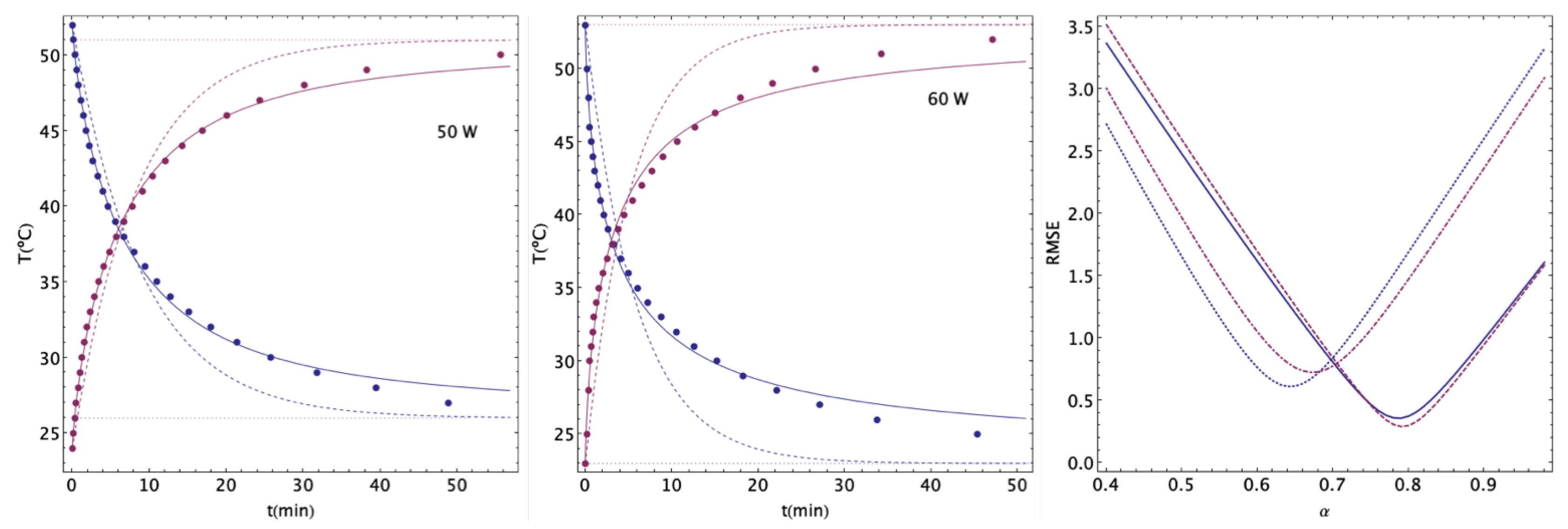
and $\mathsf{\Gamma }\left(z\right)$ stands for the gamma function [27]. In Figure 3, we plot the variation of the temperature values measured for 50 W and 60 W LED chips in horizontal configuration (the axis of symmetry of the sink is perpendicular to the gravity force) corresponding to situations analogous to that of Figure 2, with the chip placed at the bottom of the heat sink. The luminaire for the 60 W is of larger size, in order to allow for a better dissipation of the produced heat. In the figure, we compare the results with fits to the simplest form of Newton’s law of cooling $T\left(t\right)=T_f+(T\left(0\right)-T_f)exp(-rt)$ and its (Caputo) fractional generalization, Equation (5). The values of $\mathsf{\alpha }$ that optimise the fits in each case are $\mathsf{\alpha }=0.79$ for heating and cooling with 50 W, $\mathsf{\alpha }=0.64$ for the cooling process with 60 W, and $\mathsf{\alpha }=0.67$ for the heating one.

The fitting of the Mittag–Leffler curves to the experimental results is good, except for small deviations at late times. A relevant question arises: why should the fractional derivative lead to better results than the conventional derivative in this setup? Following [19], our conjecture is that this happens because there are several relaxation rates at play. The conventional derivative is local in time but the fractional derivatives integrate over a time interval, opening the possibility of taking into account a more complex type of temporal dynamics. In fact, we checked that fits of the type

$$T\left(t\right)=T_f+\sum _i{A}_{i}exp(-r_{i}t)$$

(7)

are excellent descriptions of the data at the expense of introducing a larger number of parameters in the fit. The fractional derivative seems to provide a simplified compact approximation to this kind of thermal dynamics. The value of $\mathsf{\alpha }$ should be related to the strength of the interplay between the different modes, approaching 1 when one of them is largely dominant. In fact, $\mathsf{\alpha }=1$ was found to be fine for metal alloy slabs in [19]. In our case, the “fractionalization” does not come from the material itself but from the nontrivial geometry of the system under study [28]. This interpretation also leads to a heuristical understanding of why the Mittag–Leffler fit gets worse at late times, when only the term with smaller $r_i$ in Equation (7) survives. Checking the validity of these qualitative statements would be an interesting problem for the future.

The possibility of fractional calculus playing a role in the thermal evolution of nontrivial systems is a compelling result, see also the aforementioned reference [19]. This can be specially important for procedures with industrial relevance. Complex material structures, in general, should not be expected to follow the simple version of Newton’s law of cooling. It is natural to conjecture that the generalization discussed here can be a powerful tool in a variety of situations. The value of the fractional derivative order $\mathsf{\alpha }$ somehow accounts for the complicated processes that determine the evolution of the system as a whole. These questions certainly require further study and we hope that this work will open new avenues in the mathematical modeling of LED luminaires.

4. Conclusions and Outlook

In this article, we analyzed the heating and cooling processes in quasi-two-dimensional LED luminaires from the point of view of mathematical modeling. We show that the steady-state temperature distribution can be accurately described by the solution of the system of equations that describes heat transfer in the aluminum passive heat sink and the surrounding air, proving that the maximal temperature of the system, which is that reached by the chip itself, can be kept well below its threshold of damage. Generalizing this kind of modeling to other situations can provide insights, saving time and resources in the fabrication process. Since the simulation quite accurately captures the measured result, it can provide a starting point to modify different geometrical parameters of the heat sink to understand how to further reduce the stationary chip temperature or how to tune the design in order to reduce costs. Another interesting possibility is to apply a similar analysis to situations with LED dimming with pulse width modulation [29], taking into account that temperature can affect the emission spectrum [30].

On the other hand, by analyzing the evolution in time of the temperature of the chip, we found that the measured $T\left(t\right)$ curves can be adequately fitted by the solution of a simple FODE. This novel application of fractional calculus in the present context might be just a curiosity, but it provides a strong motivation to revisit the study of the thermal dynamics of systems with complex spatial profiles from this point of view.

An interesting research avenue beyond the scope of the present work would be to combine both approaches and to solve the full three-dimensional time-dependent set of equations in order to determine from first principles the time evolution of the chip temperature and then compare it to simple effective models based on FODEs. This could shed light both on the thermal dynamics of the system and on the way in which FODEs can emerge as simplified descriptions of certain aspects of complex physical systems. The scope of applicability of FODEs for similar systems is an interesting question to be addressed in the future. We hope that this contribution will pave the way for new approaches involving fractional calculus for the mathematical modeling of physical systems of industrial interest.