Impact on Stability by the Use of Memory in Traub-Type Schemes

Abstract

In this work, two Traub-type methods with memory are introduced using accelerating parameters. To obtain schemes with memory, after the inclusion of these parameters in Traub’s method, they have been designed using linear approximations or the Newton’s interpolation polynomials. In both cases, the parameters use information from the current and the previous iterations, so they define a method with memory. Moreover, they achieve higher order of convergence than Traub’s scheme without any additional functional evaluations. The real dynamical analysis verifies that the proposed methods with memory not only converge faster, but they are also more stable than the original scheme. The methods selected by means of this analysis can be applied for solving nonlinear problems with a wider set of initial estimations than their original partners. This fact also involves a lower number of iterations in the process.

1. Introduction

Finding the solution of a nonlinear equation $f\left(x\right)=0$ has been and still is present in many fields of Technology and Science. Because many of these equations cannot be solved analytically, the solution of this kind of problems is approximated by using iterative methods. Among them, the best-known is Newton’s scheme, with quadratic convergence under some conditions.

The role of iterative processes for solving nonlinear problems of many branches of science and engineering has increased exponentially in recent years. This is due to the applicability of these algorithms to real life problems. For instance, Shacham et al. [1,2], described the fraction of the nitrogen-hydrogen feed that gets converted to ammonia (this fraction is known as fractional conversion) in the form of nonlinear scalar equation. On the other hand, Shacham [3] described the fractional conversion in a chemical reactor also by using a scalar equation. Moreover, Shacham and Kehat [4] gave several examples of real life problems which are modeled by means of nonlinear scalar equation such as: chemical equilibrium calculations problem, energy or material balance problem in a chemical reactor problem, isothermal flash problem, azeotropic point calculation problem, calculation of gas volume from Beattie Bridgeman problem, adiabatic flame temperature problem, liquid flow rate in pipe problem, pressure drop in a converging diverging nozzle problem, etc.

There is an extensive literature related to iterative methods for solving nonlinear equations. The design of new efficient methods is an ongoing issue for scientists. Recently, this design goes hand to hand with the dynamical analysis [5,6,7,8,9], allowing the knowledge of the stability of the methods involved.

Kung and Traub conjectured in [10] that iterative methods without memory which use d functional evaluations per iteration cannot have order of convergence higher than $2^{d-1}$. The inclusion of the memory in the iterative methods is a powerful technique, since it increases the order of convergence of the method without adding new functional evaluations. Traub designed the first method with memory [11] based on the Steffensen’s one [12], increasing the order of convergence from 2 to $2.41$. Several authors have modified the iterative methods to include memory, as done in [13] for methods with derivatives, or [14,15,16] for derivative-free ones.

In this work, we focus on the order of convergence of two Traub-type methods when we modify its iterative expression to obtain methods with memory. Moreover, the dynamical analysis is performed in a similar way as done in [17,18,19,20].

To analyze the order of convergence of each method with memory, we use the following result [21]:

Theorem 1.

Let φ be an iterative method with memory that generates a convergent sequence$\left\{x_k\right\}$of approximations of a zero α of function f. Let us assume a nonzero constant τ and positive numbers$p_i$,$i=0,1,\dots ,m$, such that

$$|e_{k+1}|\le \tau \prod _{i=0}^m{|e_{k-i}|}^{p_i}$$

holds. Then, the R-order of convergence of φ satisfies

$$O_R(\phi ,\alpha )\ge p,$$

being p the only positive root of the polynomial

$$p^{m+1}-\sum _{i=0}^m{p}_i{p}^{m-i}.$$

The rest of this manuscript is organized as follows. In Section 2, the basic concepts of dynamics for both one-dimensional and multidimensional real cases are remembered, since the analysis of iterative methods with memory requires the multidimensional dynamics for real variable. Based on Traub’s method, Section 3 collects the construction of two new methods with memory. The first scheme needs two previous iterations, while the second one also needs an intermediate point. The convergence of the methods without and with memory is also performed. To analyze the stability of the introduced methods, Section 4 is devoted to the dynamical study. Finally, some discussion and conclusions about the results are presented in Section 5.

2. Real Dynamics

The study of the dynamical properties of the rational operator associated with an iterative scheme on low degree polynomials, gives interesting information about the stability of this method. This study is usually carried out applying tools of complex dynamics. However, as stated in [22], the knowledge of the complex dynamics is not included in the study of the real dynamics, since the behavior can be different. Therefore, when we have an iterative method with memory, the fundamentals of the complex dynamics can be applied, but they must be particularized for the real variable case.

The aim of this paper is to compare an iterative scheme without memory with other two schemes with memory that have been obtained from the first one. Then, we will focus on tools of real dynamics distinguishing the one-dimensional case, used for real dynamics without memory, from the multidimensional case, used in real dynamics of methods with memory.

When an iterative method is applied on a nonlinear equation $f\left(x\right)=0$, we obtain a rational function whose dynamics are unknown. Now we recall some basic concepts of real dynamics for the one-dimensional case. To expand these contents see, for example [23,24].

Let $R:\mathbb{R}⟶\mathbb{R}$ be the rational function obtained when an iterative scheme is applied on a polynomial $f\left(x\right)$. Then, the orbit of a point $x_0\in \mathbb{R}$ is given by $\{x_0,R\left(x_0\right),R^2\left(x_0\right),\dots \}$. A fixed point $x^F$ of R satisfies $R\left(x^F\right)=x^F$. It is called strange fixed point when it does not coincide with a root of $f\left(x\right)$. Moreover, a point $x_0$ is a T-periodic point when $R^T\left(x_0\right)=x_0$ but $R^t\left(x_0\right)\ne x_0$, $t<T$, where $T,t\in \mathbb{N}$. A fixed point is T-periodic with $T=1$.

The stability of the fixed points depends on the multiplier of the fixed point, $|R^{\prime }\left(x\right)|$, when $R^{\prime }$ denotes the derivative of function R. Therefore, if $x^F\in \mathbb{R}$ is a fixed point of R, it is called attracting when $|R^{\prime }\left(x^F\right)|<1$; repelling if $|R^{\prime }\left(x^F\right)|>1$; superattracting if $|R^{\prime }\left(x^F\right)|=0$; and neutral when $|R^{\prime }\left(x^F\right)|=1$.

A critical point $x^C$ holds $R\left(x^C\right)=0$, and it is called free critical point when it is different from the roots of $f\left(x\right)$.

When $x^F$ is an attracting fixed point, we define the basin of attraction as the set of pre-images of any order such that

$$\mathcal{A}\left(x^F\right)=\{x_0\in \mathbb{R}:R^n\left(x_0\right)⟶x^F,n⟶\infty \}.$$

Iterative schemes which use two previous iterations to calculate the following iterate have the general form $x_{k+1}=h(x_{k-1},x_k)$, $k\ge 1$, being $x_0$ and $x_1$ two initial estimations. To carry out the dynamical study of a method with memory, we need to build an associated discrete dynamical system [17]. For this purpose, we consider the auxiliary function $\mathbf{G}:{\mathbb{R}}^2⟶{\mathbb{R}}^2$ defined as

$$\mathbf{G}(x_{k-1},x_k)=(x_k,x_{k+1})=(x_k,h(x_{k-1},x_k)),k\ge 1.$$

Please note that this definition can be easily adapted to schemes with memory which use more than two previous iterations in each step.

As we did in the one-dimensional case, we recall on some dynamical concepts. A point $(z,x)\in {\mathbb{R}}^2$ is a fixed point of $\mathbf{G}$ when it satisfies $\mathbf{G}(z,x)=(z,x)$. So, it must verify $z=x$ and $x=h(z,x)$. When a fixed point $(z,x)$ does not agree with a root of $f\left(x\right)$, it is called strange fixed point.

As in complex dynamics, the orbit of a point ${\mathbf{x}}_{\mathbf{0}}\in {\mathbb{R}}^2$ is composed of its successive images by $\mathbf{G}$

$$\{{\mathbf{x}}_{\mathbf{0}},\mathbf{G}\left({\mathbf{x}}_{\mathbf{0}}\right),\dots ,{\mathbf{G}}^m\left({\mathbf{x}}_{\mathbf{0}}\right),\dots \},$$

and its dynamical behavior can be classified depending on its asymptotical behavior. Hence, ${\mathbf{x}}_{\mathbf{0}}\in {\mathbb{R}}^2$ is a T-periodic point when ${\mathbf{G}}^T\left({\mathbf{x}}_{\mathbf{0}}\right)={\mathbf{x}}_{\mathbf{0}}$ but ${\mathbf{G}}^t\left({\mathbf{x}}_{\mathbf{0}}\right)\ne {\mathbf{x}}_{\mathbf{0}}$, for $t<T$.

The stability of the fixed points of $\mathbf{G}$ can be analyzed using the following result [25]:

Theorem 2.

Let$\mathbf{G}:{\mathbb{R}}^n⟶{\mathbb{R}}^n$be of class${\mathcal{C}}^2$and${\mathbf{x}}^{\mathbf{T}}$a T-periodic point. Let${\lambda }_1,{\lambda }_2,\dots ,{\lambda }_n$be the eigenvalues of${\mathbf{G}}^{\prime }\left({\mathbf{x}}^{\mathbf{T}}\right)$, where$G^{\prime }$is the Jacobian matrix of G.

(a) 

If$|{\lambda }_j|<1$, for$j=1,2,\dots ,n$, then${\mathbf{x}}^{\mathbf{T}}$is attracting.

(b) 

If one eigenvalue${\lambda }_{j_0}$has$|{\lambda }_{j_0}|>1$, then${\mathbf{x}}^{\mathbf{T}}$is repelling or saddle.

(c) 

If$|{\lambda }_j|>1$, for$j=1,2,\dots ,n$, then${\mathbf{x}}^{\mathbf{T}}$is repelling.

Moreover, if $|{\lambda }_j|\ne 1$, for $j=1,2,\dots ,n$, ${\mathbf{x}}^{\mathbf{T}}$ is hyperbolic. In particular, if there exists an eigenvalue such that $|{\lambda }_i|<1$ and another such that $|{\lambda }_j|>1$, the hyperbolic point is called saddle point. Please note that for $T=1$, the T-periodic point is recalled as fixed point, and it is denoted by ${\mathbf{x}}^{\mathbf{F}}$.

Finally, the basin of attraction of a T-periodic point ${\mathbf{x}}^{\mathbf{T}}$ is defined as:

$$\mathcal{A}\left({\mathbf{x}}^{\mathbf{T}}\right)=\{{\mathbf{x}}_{\mathbf{0}}\in {\mathbb{R}}^n:G^m\left({\mathbf{x}}_{\mathbf{0}}\right)⟶{\mathbf{x}}^{\mathbf{T}},m\to \infty \}.$$

3. Traub-Type Methods with Memory

The well-known Traub’s method [11] has the iterative expression

$$\begin{array}{cc}\hfill y_k=& x_k-\frac{f\left(x_k\right)}{f^{\prime }\left(x_k\right)},\hfill \\ \hfill x_{k+1}=& y_k-\frac{f\left(y_k\right)}{f^{\prime }\left(x_k\right)}.\hfill \end{array}$$

(1)

The next result shows the order of convergence of the method from its error equation.

Theorem 3.

Let us consider a real function$f:I\subset \mathbb{R}⟶\mathbb{R}$, sufficiently differentiable in an open interval I. If$\alpha \in I$is a simple zero of f and$x_0$is near enough to α, then sequence$\left\{x_k\right\}$generated by Traub’s method (1) converges to α with order of convergence 3, being its error equation:

$$e_{k+1}=2c_2^2{e}_k^3+\mathcal{O}\left(e_k^4\right).$$

where $e_k=x_k-\alpha$ and $c_j=\frac{f^{\left(j\right)}\left(\alpha \right)}{j!f^{\prime }\left(\alpha \right)}$, $j\ge 2$.

Although in Traub’s scheme is not possible to increase the order of convergence, some changes on its iterative expression allow us the inclusion of memory, obtaining methods with higher order of convergence.

To improve the order in Traub’s method, we start by adding an accelerator parameter $\delta$ in the first step of its iterative scheme, so we obtain:

$$\begin{array}{cc}\hfill y_k=& x_k-\frac{f\left(x_k\right)}{f^{\prime }\left(x_k\right)+\delta f\left(x_k\right)},\hfill \\ \hfill x_{k+1}=& y_k-\frac{f\left(y_k\right)}{f^{\prime }\left(x_k\right)}.\hfill \end{array}$$

(2)

The order of convergence of the resulting family is set in the following result.

Theorem 4.

Let us consider a real function$f:I\subset \mathbb{R}⟶\mathbb{R}$, sufficiently differentiable in an open interval I. If$\alpha \in I$is a simple zero of f and$x_0$is near enough to α, then the iterative family (2) converges to α with order of convergence 3 for any value of parameter δ, being its error equation

$$e_{k+1}=2c_2(c_2+\delta )e_k^3+\mathcal{O}\left(e_k^4\right),$$

(3)

where $e_k=x_k-\alpha$ and $c_j=\frac{f^{\left(j\right)}\left(\alpha \right)}{j!f^{\prime }\left(\alpha \right)}$, $j\ge 2$.

Proof. 

By using Taylor series expansions, $f\left(x_k\right)$ can be expressed as

$$f\left(x_k\right)=f^{\prime }\left(\alpha \right)\left[e_k+c_2{e}_k^2+c_3{e}_k^3+c_4{e}_k^4\right]+\mathcal{O}\left(e_k^5\right),$$

and its derivative

$$f^{\prime }\left(x_k\right)=f^{\prime }\left(\alpha \right)\left[1+2c_2{e}_k+3c_3{e}_k^2+4c_4{e}_k^3\right]+\mathcal{O}\left(e_k^4\right).$$

By using these expansions, we have

$$y_k-\alpha =e_k-\frac{f\left(x_k\right)}{f^{\prime }\left(x_k\right)+\delta f\left(x_k\right)}=\left(c_2+\delta \right)e_k^2+\left(-2c_2\delta -2c_2^2+2c_3-{\delta }^2\right)e_k^3+\mathcal{O}\left(e_k^4\right),$$

and

$$\begin{array}{ccc}\hfill f\left(y_k\right)& =& f^{\prime }\left(\alpha \right)\left[y_k-\alpha +c_2{(y_k-\alpha )}^2+c_3{(y_k-\alpha )}^3\right]+\mathcal{O}({(y_k-\alpha )}^4)\hfill \\ & =& f^{\prime }\left(\alpha \right)\left[(c_2+\delta )e_k^2+\left(-2c_2\delta -2c_2^2+2c_3-{\delta }^2\right)e_k^3\right]+\mathcal{O}\left(e_k^4\right).\hfill \end{array}$$

Then, we obtain the following error equation

$$e_{k+1}=y_k-\alpha -\frac{f\left(y_k\right)}{f^{\prime }\left(x_k\right)}=2c_2(c_2+\delta )e_k^3+\mathcal{O}\left(e_k^4\right).$$

 ☐

We study how to increase the order of the class by analyzing its error equation. If $\delta =-c_2=-{\displaystyle \frac{f^{″}\left(\alpha \right)}{2f^{\prime }\left(\alpha \right)}}$ the order increases in, at least, one unit. Unfortunately, $\alpha$ is not known. Therefore, we need to approximate $f^{\prime }\left(\alpha \right)$ and $f^{″}\left(\alpha \right)$ transforming the iterative schemes in other ones with memory.

If the following linear approximations are applied

$$\begin{array}{cc}{f}^{\prime }\left(\alpha \right)\approx f^{\prime }\left(x_k\right),\hfill & f^{″}\left(\alpha \right)\approx \frac{f^{\prime }\left(x_k\right)-f^{\prime }\left(x_{k-1}\right)}{x_k-x_{k-1}},\hfill \end{array}$$

(4)

the accelerator parameter gets into

$$\begin{array}{c}\hfill {\delta }_k\approx -\frac{1}{2}\frac{f^{\prime }\left(x_k\right)-f^{\prime }\left(x_{k-1}\right)}{(x_k-x_{k-1})f^{\prime }\left(x_k\right)}.\end{array}$$

(5)

Then, we have an iterative scheme with memory whose order of convergence is analyzed below. For simplicity, the Traub-type method with memory (2) with ${\delta }_k$ defined by (5) will be denoted by TM1.

Theorem 5.

Let us consider a real function$f:I\subset \mathbb{R}⟶\mathbb{R}$, sufficiently differentiable in an open interval I. If$\alpha \in I$is a simple zero of f and$x_0$is near enough to α, then the iterative method TM1 converges to α with order of convergence$p\approx 3.30$, and its error equation is:

$$e_{k+1}=-3c_2{c}_3{e}_{k-1}{e}_k^3+{\mathcal{O}}_4(e_k,e_{k-1}),$$

where${\mathcal{O}}_4(e_k,e_{k-1})$indicates that the sum of the exponents of$e_k$ and $e_{k-1}$ in the rejected terms of the development is at least 4.

Proof. 

From the error Equation (3), the following relation is satisfied

$$e_{k+1}\sim 2c_2(c_2+{\delta }_k)e_k^3+\mathcal{O}\left(e_k^4\right).$$

By using Taylor series expansions, we have

$$\begin{array}{ccc}\hfill f\left(x_k\right)& =& f^{\prime }\left(\alpha \right)\left[e_k+c_2{e}_k^2+c_3{e}_k^3+c_4{e}_k^4\right]+\mathcal{O}\left(e_k^5\right),\hfill \\ \hfill f\left(x_{k-1}\right)& =& f^{\prime }\left(\alpha \right)\left[e_{k-1}+c_2{e}_{k-1}^2+c_3{e}_{k-1}^3+c_4{e}_{k-1}^4\right]+\mathcal{O}\left(e_{k-1}^5\right),\hfill \end{array}$$

and

$$\begin{array}{ccc}\hfill f^{\prime }\left(x_k\right)& =& f^{\prime }\left(\alpha \right)\left[1+2c_2{e}_k+3c_3{e}_k^2+4c_4{e}_k^3\right]+\mathcal{O}\left(e_k^4\right),\hfill \\ \hfill f^{\prime }\left(x_{k-1}\right)& =& f^{\prime }\left(\alpha \right)\left[1+2c_2{e}_{k-1}+3c_3{e}_{k-1}^2+4c_4{e}_{k-1}^3\right]+\mathcal{O}\left(e_{k-1}^4\right).\hfill \end{array}$$

Therefore, the accelerator parameter is

$$\begin{array}{ccc}\hfill {\delta }_k& =& -\frac{1}{2}\frac{f^{\prime }\left(x_k\right)-f^{\prime }\left(x_{k-1}\right)}{(e_k-e_{k-1})f^{\prime }\left(x_k\right)}\hfill \\ & =& -c_2-\frac{3}{2}{c}_3{e}_{k-1}+\left(2c_2^2-\frac{3}{2}{c}_3\right)e_k+(3c_2{c}_3-2c_4)e_{k-1}{e}_k-2c_4{e}_{k-1}^2+(-4c_2^3+6c_2{c}_3-2c_4)e_k^2\hfill \\ & & +{\mathcal{O}}_3(e_k,e_{k-1}).\hfill \end{array}$$

By taking the lower order terms,

$${\delta }_k+c_2\sim -\frac{3}{2}{c}_3{e}_{k-1}.$$

Then, we obtain

$$e_{k+1}\sim 2c_2\left(-\frac{3}{2}{c}_3{e}_{k-1}\right)e_k^3\sim e_{k-1}{e}_k^3.$$

(6)

Let the R-order of the method be at least p. Then it is satisfied

$$e_{k+1}\sim D_{k,p}{e}_k^p,$$

where $D_{k,p}$ tends to the asymptotic error constant, $D_p$, when $k⟶\infty$. Analogously,

$$e_k\sim D_{k-1,p}{e}_{k-1}^p.$$

Then, we have

$$e_{k+1}\sim D_{k,p}{\left(D_{k-1,p}{e}_{k-1}^p\right)}^p=D_{k,p}{D}_{k-1,p}^p{e}_{k-1}^{p^2}.$$

(7)

In the same way, relation (6) satisfies

$$e_{k+1}\sim e_{k-1}{\left(D_{k-1,p}{e}_{k-1}^p\right)}^3=D_{k-1,p}^3{e}_{k-1}^{3p+1}.$$

(8)

Finally, the exponents of $e_{k-1}$ in (7) and (8) must be the same, so it is obtained the following equation:

$$p^2=3p+1.$$

In the previous equation the only positive solution $p\approx 3.30$ gives the order of convergence of the method. ☐

Based on Theorem 5, the inclusion of memory increases the order of convergence of the family, since the order of convergence of (1) and (2) has lower values. In Section 4.2 the dynamical study of this family is performed, to check the stability of its members.

Following an analogous way to proceed as in the TM1 case, two accelerating parameters ${\delta }_1$ and ${\delta }_2$ are included in Traub’s original method (1) obtaining the iterative scheme

$$\begin{array}{cc}\hfill y_k=& x_k-\frac{f\left(x_k\right)}{f^{\prime }\left(x_k\right)+{\delta }_{1}f\left(x_k\right)},\hfill \\ \hfill x_{k+1}=& y_k-\frac{f\left(y_k\right)}{f^{\prime }\left(x_k\right)+{\delta }_{2}f\left(x_k\right)},k=0,1,\dots \hfill \end{array}$$

(9)

whose error equation is shown in the next result.

Theorem 6.

Let us consider a real function$f:I\subset \mathbb{R}⟶\mathbb{R}$, sufficiently differentiable in an open interval I. If$\alpha \in I$is a simple zero of f and$x_0$is near enough to α, then the iterative family (9) has order of convergence 3, for any values of parameters ${\delta }_1$ and ${\delta }_2$, and its error equation is:

$$e_{k+1}=({\delta }_1+c_2)({\delta }_2+2c_2)e_k^3+\mathcal{O}\left(e_k^4\right),$$

(10)

where $e_k=x_k-\alpha$ and $c_j=\frac{f^{\left(j\right)}\left(\alpha \right)}{j!f^{\prime }\left(\alpha \right)}$, $j\ge 2$.

Proof. 

By using Taylor series expansions around the root $\alpha$, $f\left(x_k\right)$ is expressed as

$$f\left(x_k\right)=f^{\prime }\left(\alpha \right)\left[e_k+c_2{e}_k^2+c_3{e}_k^3+c_4{e}_k^4\right]+\mathcal{O}\left(e_k^5\right),$$

and its derivative

$$f^{\prime }\left(x_k\right)=f^{\prime }\left(\alpha \right)\left[1+2c_2{e}_k+3c_3{e}_k^2+4c_4{e}_k^3\right]+\mathcal{O}\left(e_k^4\right).$$

Using these expansions, we have

$$\begin{array}{ccc}\hfill y_k-\alpha & =& e_k-\frac{f\left(x_k\right)}{f^{\prime }\left(x_k\right)+{\delta }_{1}f\left(x_k\right)}\hfill \\ & =& \left(c_2+{\delta }_1\right)e_k^2+\left(-2c_2{\delta }_1-2c_2^2+2c_3-{\delta }_1^2\right)e_k^3+\mathcal{O}\left(e_k^4\right).\hfill \end{array}$$

Expanding $f\left(y_k\right)$ around $\alpha$, we obtain

$$f\left(y_k\right)=f^{\prime }\left(\alpha \right)\left[(c_2+{\delta }_1)e_k^2+(-2c_2{\delta }_1-2c_2^2+2c_3-{\delta }_1^2)e_k^3\right]+\mathcal{O}\left(e_k^4\right).$$

Then, the error equation becomes

$$e_{k+1}=y_k-\alpha -\frac{f\left(y_k\right)}{f^{\prime }\left(x_k\right)+{\delta }_{2}f\left(x_k\right)}=({\delta }_1+c_2)({\delta }_2+2c_2)e_k^3+\mathcal{O}\left(e_k^4\right).$$

 ☐

If we study how to increase the order of convergence of this class, we can easily verify that if ${\delta }_1=-c_2$ and ${\delta }_2=-2c_2$ the order of convergence can increase, at least, up to 5. We need to approximate $f^{\prime }\left(\alpha \right)$ and $f^{″}\left(\alpha \right)$ and it could be done again by using linear approximations as in the family TM1. However, if we want to get an order of convergence closer to 5 it is preferable to use higher order approximations.

For this purpose, we use the Newton’s interpolation polynomial of second degree, set through three available approximations $x_k$, $x_{k-1}$ and $y_{k-1}$ to interpolate f. Denoted as $N_2(t;x_k,x_{k-1},y_{k-1})=N_2\left(t\right)$, it is defined by

$$N_2\left(t\right)=f\left(x_k\right)+f[x_k,x_{k-1}](t-x_k)+f[x_k,x_{k-1},y_{k-1}](t-x_k)(t-x_{k-1}).$$

(11)

Now, if we set the approximations

$$f^{\prime }\left(\alpha \right)\approx N_2^{\prime }\left(x_k\right),f^{″}\left(\alpha \right)\approx N_2^{″}\left(x_k\right),$$

we have the following accelerator parameters:

$${\delta }_{1,k}\approx -\frac{1}{2}\frac{N_2^{″}\left(x_k\right)}{N_2^{\prime }\left(x_k\right)},{\delta }_{2,k}\approx -\frac{N_2^{″}\left(x_k\right)}{N_2^{\prime }\left(x_k\right)}.$$

(12)

The Traub-type family with memory (9), taking the expression for the two accelerator parameters in (12), is called TM2 method.

In the next theorem, we prove how much the order has increased with respect to Traub’s method.

Theorem 7.

Let us consider a real function$f:I\subset \mathbb{R}⟶\mathbb{R}$, sufficiently differentiable in an open interval I. If$\alpha \in I$is a simple zero of f and$x_0$is near enough to α, then the iterative method TM2 converges to α with order of convergence$p\approx 3.56$.

Proof. 

From expression (10), we have the following relation

$$e_{k+1}\sim ({\delta }_{1,k}+c_2)({\delta }_{2,k}+2c_2)e_k^3.$$

(13)

Let us denote $e_{k,y}=y_k-\alpha$, for all k. Let $N_2\left(t\right)$ be defined in (11) and the following Taylor developments in terms of the errors in each iterative step of the method:

$$\begin{array}{cc}\hfill f\left(x_k\right)=& f^{\prime }\left(\alpha \right)\left[e_k+c_2{e}_k^2+c_3{e}_k^3+c_4{e}_k^4\right]+\mathcal{O}\left(e_k^5\right),\hfill \\ \hfill f\left(x_{k-1}\right)=& f^{\prime }\left(\alpha \right)\left[e_{k-1}+c_2{e}_{k-1}^2+c_3{e}_{k-1}^3+c_4{e}_{k-1}^4\right]+\mathcal{O}\left(e_{k-1}^5\right),\hfill \\ \hfill f\left(y_{k-1}\right)=& f^{\prime }\left(\alpha \right)\left[e_{k-1,y}+c_2{e}_{k-1,y}^2+c_3{e}_{k-1,y}^3+c_4{e}_{k-1,y}^4\right]+\mathcal{O}\left(e_{k-1,y}^5\right).\hfill \end{array}$$

(14)

Using these developments in $N_2\left(t\right)$, evaluating the derivatives of $N_2\left(t\right)$ in the point $x_k$ and rejecting the terms of order higher than 0 of $e_k$, we obtain:

$${\delta }_{1,k}=-c_2-c_3{e}_{k-1,y}-c_3{e}_{k-1}-c_4{e}_{k-1,y}^2-c_4{e}_{k-1}^2+(-c_2{c}_3-c_4)e_{k-1,y}{e}_{k-1}+{\mathcal{O}}_3(e_{k-1},e_{k-1,y}).$$

From the previous calculation the following relations are satisfied:

$$\begin{array}{c}{\delta }_{1,k}+c_2\sim e_{k-1}\\ {\delta }_{2,k}+2c_2=2({\delta }_{1,k}+c_2)\sim 2e_{k-1}\sim e_{k-1}.\end{array}$$

(15)

On the other hand, let the R-order of the method be at least p. So, it is satisfied

$$e_{k+1}\sim D_{k,p}{e}_k^p$$

where $D_{k,p}$ tends to $D_p$, the asymptotic error constant, when $k\to \infty$.

In the same way,

$$e_k\sim D_{k-1,p}{e}_{k-1}^p$$

(16)

so

$$e_{k+1}\sim D_{k,p}{\left(D_{k-1,p}{e}_{k-1}^p\right)}^p=D_{k,p}{D}_{k-1,p}^p{e}_{k-1}^{p^2}.$$

(17)

Using relations (15) and (16), in (13):

$$e_{k+1}\sim e_{k-1}^2{e}_k^3\sim e_{k-1}^2{\left(D_{k-1,p}{e}_{k-1}^p\right)}^3\sim e_{k-1}^{3p+2}$$

(18)

Finally, if we match the exponents of (17) and (18), the following equation is obtained:

$$p^2=3p+2$$

In this problem, the only possible solution for the previous equation is

$$p\approx 3.56.$$

Then, TM2 method has order of convergence $p\approx 3.56$. ☐

4. Stability Analysis

4.1. Real Dynamics of Traub’s Method

In [5], Amat et al. carry out a dynamical study about Traub’s method when it is applied to polynomials of second and third degree. By taking this study on quadratic polynomials as a reference, we construct and analyze the bifurcation diagrams and the dynamical lines of this method. This analysis allow us to compare the dynamical features of Traub’s method with the TM1 and TM2 corresponding ones.

Consider the next result that allows the generalization of dynamic study in some iterative schemes.

Theorem 8 (Scaling theorem).

Let$f\left(x\right)$be an analytic function, and let$A\left(x\right)=\alpha x+\beta$, with$\alpha \ne 0$, be an affine map. Let$g\left(x\right)=\lambda (f\circ A)\left(x\right)$, with$\lambda \ne 0$. Then, the fixed-point operator$M_f$is analytically conjugated to$M_g$by A, i.e.,$(A\circ M_g\circ A^{-1})\left(x\right)=M_f\left(x\right)$.

In addition, it is possible to analyze the dynamics of a family of polynomials with just the analysis of a few cases.

Theorem 9.

Let$q\left(x\right)=a_1{x}^2+a_{2}x+a_3$,$a_1\ne 0$, be a generic quadratic polynomial with simple roots. Then$q\left(x\right)$can be reduced to$p\left(x\right)=x^2+c$, where$c=4a_1{a}_3-a_2^2$, by means of an affine map. This affine transformation induces a conjugation between$M_q$and$M_p$, the fixed-point operators corresponding to polynomials$q\left(x\right)$and$p\left(x\right)$, respectively.

Traub’s method satisfies the Scaling Theorem, as proved in [5]. Moreover, according to Theorem 9, the study of the family of polynomials $p_c\left(x\right)=x^2+c$ can be generalized to any quadratic polynomial.

If we apply Traub’s method on $p_c\left(x\right)=x^2+c$, $c\in \mathbb{R}$, we obtain the fixed-point operator $M_c:\mathbb{R}⟶\mathbb{R}$ which depends on c:

$$M_c\left(x\right)=-\frac{c^2+6c{x}^2-3x^4}{8x^3}.$$

Solving $M_c\left(x\right)=x$ we get for all $c<0$ two fixed points, $x_1^F\left(c\right)=-\sqrt{-c}$ and $x_2^F\left(c\right)=\sqrt{-c}$, corresponding to the roots of $p_c\left(x\right)$, which are superattracting. Moreover, $x_3^F\left(c\right)=-\frac{\sqrt{-c}}{\sqrt{5}}$ and $x_4^F\left(c\right)=\frac{\sqrt{-c}}{\sqrt{5}}$ are two repelling strange fixed points of $M_c$ when $c<0$, since $|M_c^{\prime }\left(x_{3,4}^F\left(c\right)\right)|=6$.

By solving the equation $M_c^{\prime }\left(x\right)=0$, we get that $x_1^C\left(c\right)=-\sqrt{-c}$ and $x_2^C\left(c\right)=\sqrt{-c}$ are the only critical points of $M_c$, so Traub’s method does not have any free critical points.

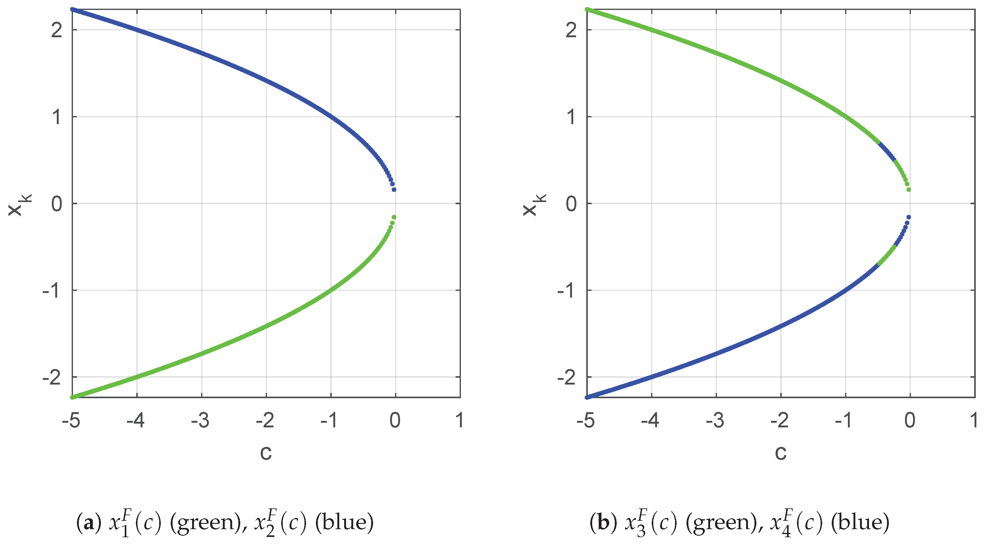
We have plotted in Figure 1 the bifurcation diagrams for the fixed points of $M_c$. Figure 1a represents the superattracting fixed points $x_1^F\left(c\right)$ and $x_2^F\left(c\right)$, while Figure 1b represents the strange fixed points $x_3^F\left(c\right)$ and $x_4^F\left(c\right)$. The plots have been generated by iterating Traub’s method taking as initial estimation the fixed points with a small perturbation. For each c, the successive values of $x_k$ are plotted from the iterate $\#500$ to $\#700$ in order to represent the advanced state of the orbit of each initial guess. The bifurcation diagrams show values of c where the method has more stability. In all cases, when $c>0$ there is no point because they are complex, so it is verified that c cannot take positive values for any fixed point. As $x_{1,2}^F\left(c\right)$ are superattracting, in Figure 1a all the points converge to one of the two roots. In Figure 1b it is observed the same behavior because $x_{3,4}^F\left(c\right)$ are repelling, so, there are not strange attracting points.

As represented in [19], the dynamical lines of Traub’s method when it is applied on $p_c\left(x\right)$ are shown in Figure 2 for different values of c. Using the software MATLAB^® 2017b, the interval $x_0\in [-5,5]$ has been divided in 500 points and they have been used as initial estimations to iterate Traub’s method. When a point in the interval converges to one of the roots of $p_c\left(x\right)$ it is painted in orange or blue. Orange points correspond to the basin of attraction of $x_1^F\left(c\right)$, while the blue ones belong to $x_2^F\left(c\right)$. It is painted in black the points that do not converge to any root. The stopping criteria are 50 maximum of iterations and a difference between two consecutive iterations of ${10}^{-3}$.

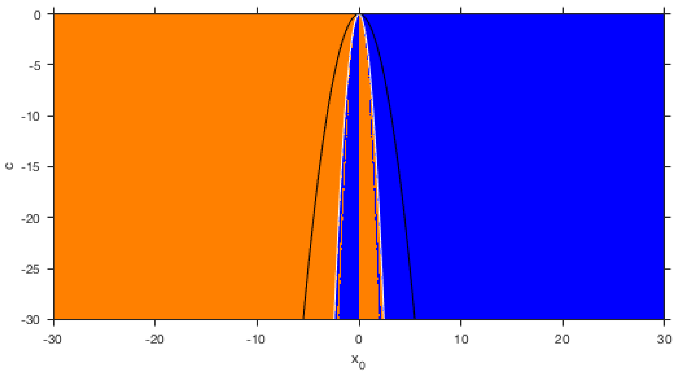
The convergence plane [26] gathers into one graphic the complete behavior of every member of a family of one-dimensional iterative methods. Figure 3 shows the convergence plane of Traub’s method. The basins of attraction of the fixed points have been colored in blue or orange taking values for the parameter $c\in \left[-30,0\right]$ and initial estimations for the method in $x_0\in \left[-30,30\right]$. As an added value, the superattracting fixed points and the strange fixed points are also represented with black and white lines, respectively, since they depend on the value of c.

For every value of $c<0$, each initial guess converges to a superattracting fixed point. Almost every initial guess of $x_0>0$ tends to $x_1^F\left(c\right)$, and almost every initial guess of $x_0<0$ tends to $x_2^F\left(c\right)$. There is a thin region of initial estimations that converge to the further superattracting fixed point. The width of this region is set by the value of the strange fixed points $x_3^F\left(c\right)$ and $x_4^F\left(c\right)$.

4.2. Multidimensional Real Dynamics of TM1 Method

From now on, we apply TM1 scheme on the family of polynomials $p_c\left(x\right)=x^2+c$. As TM1 is a method with memory, its fixed-point function depends on the two previous iterates, $x_k$ and $x_{k-1}$, that will be denoted by x and z, respectively. Then the fixed-point function is:

$${\mathbf{R}}_{\mathbf{c}}(z,x)=(x,g(z,x))=\left(x,-\frac{4x^2{z}^4+8c{x}^2{z}^2-9x^6+15c{x}^4-3c^2{x}^2+c^3}{2x{(c-3x^2)}^2}\right).$$

Since a fixed point must satisfy $z=x$ and $x=g(z,x)$, the fixed points are these x such that ${\mathbf{R}}_{\mathbf{c}}(x,x)=(x,x)$. Solving this equation, the only fixed points for $c\le 0$ are the roots of $p_c\left(x\right)$, ${\mathbf{x}}_{\mathbf{1},\mathbf{2}}^{\mathbf{F}}\left(c\right)=(\pm \sqrt{-c},\pm \sqrt{-c})$. When $c>0$ all the fixed points are complex, so they are out of this study.

To analyze the behavior of the fixed points, let us consider the Jacobian matrix of ${\mathbf{R}}_{\mathbf{c}}(z,x)$ at the point ${\mathbf{x}}_{\mathbf{1}}^{\mathbf{F}}\left(c\right)=(-\sqrt{-c},-\sqrt{-c})$:

$${\mathbf{R}}_{\mathbf{c}}^{\prime }(-\sqrt{-c},-\sqrt{-c})=\left(\begin{array}{cc}0& 1\\ 0& 0\end{array}\right).$$

The eigenvalues associated with this fixed point are ${\lambda }_1={\lambda }_2=0$. The same result is obtained with the fixed point ${\mathbf{x}}_{\mathbf{2}}^{\mathbf{F}}\left(c\right)=(\sqrt{-c},\sqrt{-c})$. Then, by applying Theorem 2, the two fixed points are attracting.

In Figure 4 some dynamical planes associated with TM1 method for different c are shown. The implementation of these dynamical planes has followed a similar structure as [27] presents. It has been used a mesh of $500\times 500$ estimations to iterate the method. Finally, each point is painted according to the root that it has converged to: blue for $(-\sqrt{-c},-\sqrt{-c})$, orange for $(\sqrt{-c},\sqrt{-c})$, and black in other case. The stopping criteria are 50 maximum of iterations and a difference between two consecutive iterations of ${10}^{-3}$. An expanding behavior of the basins of attraction can be seen when the value of c decreases. Let us remark that there is not any periodic orbit in the black region.

4.3. Multidimensional Real Dynamics of TM2 Method

As stated in Section 2, methods with memory that use two previous iterates have the expression $x_{k+1}=g(x_{k-1},x_k)$. However, as TM2 method uses the interpolation polynomial $N_2(t;x_k,x_{k-1},y_{k-1})$, the calculation of the estimation $x_{k+1}$ requires the knowledge of $x_k$, $x_{k-1}$ and $y_{k-1}$. Therefore, the general expression of a method with memory that uses three previous points is

$$x_{k+1}=g(x_{k-1},y_{k-1},x_k),k\ge 1,$$

being g its fixed-point function. Moreover, its fixed-point operator $\mathbf{G}:{\mathbb{R}}^3⟶{\mathbb{R}}^3$ is defined by the expression

$$\mathbf{G}(x_{k-1},y_{k-1},x_k)=(x_k,y_k,x_{k+1})=(x_k,y_k,g(x_{k-1},y_{k-1},x_k)),k=1,2,\dots ,$$

(19)

where $x_0$, $y_0$ and $x_1$ are the initial approximations.

It will be denoted $x=x_k$, $z=x_{k-1}$, $xy=y_k$ and $zy=y_{k-1}$, for all k. Then, (19) defines a discrete dynamical system whose fixed points $(z,zy,x)\in {\mathbb{R}}^3$ must verify

$$z=zy=x,x=g(z,zy,x).$$

(20)

To compare the stability of TM2 with TM1 and Traub (1) methods, the family of polynomials $p_c\left(x\right)=x^2+c$ is used again. The fixed-point operator of TM2 scheme, when it is applied on $p_c\left(x\right)$, is

$${\mathbf{G}}_{\mathbf{c}}(z,zy,x)=\left(x,xy,-\frac{2x(-2c^3+5c^2{x}^2-8c{x}^4+x^6)}{{(c-3x^2)}^2(c-x^2)}\right).$$

(21)

Since the conditions (20) are imposed to ${\mathbf{G}}_c$ in order to obtain a real-valued function, the result is a one-dimensional operator ${\tilde{G}}_c\left(x\right)$. The analysis of the stability of its fixed points requires the dynamical analysis. For this purpose, the one-dimensional operator gets the expression

$${\left[{\mathbf{G}}_{\mathbf{c}}(z,zy,x)\right]}_{{\mid }_{z=zy=x}}={\tilde{G}}_c\left(x\right)=-\frac{2x(-2c^3+5c^2{x}^2-8c{x}^4+x^6)}{{(c-3x^2)}^2(c-x^2)}.$$

The fixed points of ${\tilde{G}}_c\left(x\right)$ are the roots of $p_c\left(x\right)$, $x_1^F\left(c\right)=-\sqrt{-c}$ and $x_2^F\left(c\right)=\sqrt{-c}$, for $c<0$. In addition, $x_3^F=0$ is a strange fixed point. When $c>0$, all the fixed points of ${\tilde{G}}_c\left(x\right)$ are complex, so they are out of the real dynamics analysis. As the Jacobian matrix is of the form

$${\mathbf{G}}_{\mathbf{c}}^{\prime }(z,zy,x)=\left(\begin{array}{ccc}0& 0& 1\\ 0& 0& 0\\ 0& 0& {\tilde{G}}_c^{\prime }\left(x\right)\end{array}\right),$$

the stability of the fixed points can be checked in ${\tilde{G}}_c^{\prime }\left(x\right)$, which is given by

$${\tilde{G}}_c^{\prime }\left(x\right)=\frac{2(2c-3x^2){(c+x^2)}^4}{{(c-3x^2)}^3{(c-x^2)}^2}.$$

By evaluating the fixed points in $|{\tilde{G}}_c^{\prime }\left(x\right)|$, $x_1^F\left(c\right)$ and $x_2^F\left(c\right)$ are superattracting, and $x_3^F$ is repelling, because $|{\tilde{G}}_c^{\prime }\left(x\right)|=4$.

Computing ${\tilde{G}}_c^{\prime }\left(x\right)=0$, four critical points are obtained: the roots of $p_c$ and two free critical points, $x_1^C\left(c\right)=-\sqrt{\frac{2}{3}c}$ and $x_2^C\left(c\right)=\sqrt{\frac{2}{3}c}$, when $c>0$.

Following the same procedure as in Traub’s method, in Figure 5 the bifurcation diagrams for the fixed points have been plotted. On the one hand, Figure 5a confirm that $x_{1,2}^F\left(c\right)$ are superattracting fixed points when $c<0$. On the other hand, Figure 5b illustrates that $x_3^F$ is a repelling point because if it is taken with a small perturbation as an initial estimation of the method, the successive iterates do not converge to it and they converge to the roots of $p_c\left(x\right)$.

The parameter lines of a method show the final orbit of each critical point depending on c. As each point of the lines represents a particular method, they allow the choice of the value of the parameter that guarantees convergence to any of the roots, i.e., the selection of the more stable methods of the family. TM2 method only has critical points when $c>0$. However, in this case there are no fixed points. For this reason, the parameter lines in TM2 method do not give us information about the stability of the family.

Figure 6 shows the dynamical lines of TM2 method when it is applied on $p_c\left(x\right)$ varying the value of c. The parameters of the representation follow the same structure as the dynamical lines of Figure 2. Figure 6a–c show that for every $c<0$, the orbit of each initial $x_0$ converges to a root of $p_c\left(x\right)$. Moreover, negative initial guesses converge to $x_1^F\left(c\right)$ and the positive ones converge to $x_2^F\left(c\right)$. As expected, TM2 method does not converge when c is positive as shown in Figure 6d.

To analyze the dynamical behavior of the complete family, Figure 7 plots the convergence plane of TM2 method. According to the notation followed in Figure 3, now there is a white line which represents $x_3^F$. The strange fixed point splits the plane into two half-planes, each one containing a different basin of attraction.

5. Conclusions

In this paper, two Traub-type iterative schemes are designed by introducing accelerating parameters in the iterative expression of Traub’s scheme. The use of memory in these parameters originates TM1 and TM2 methods, whose convergence analysis and stability have been carried out to compare them with Traub’s scheme.

In the dynamical study, Traub and TM1 methods have strange fixed points but their bifurcation diagrams show that they are repelling. In addition, it can be checked in the bifurcation diagrams that the roots of $p_c\left(x\right)$ are superattracting points because the iterates, although they are close to a strange fixed point, converge to one of them.

In the analysis of the order of convergence in Traub, TM1 and TM2 methods, the use of memory guarantees higher order of convergence than the original method without any additional functional evaluations. Moreover, the convergence plane in Figure 7 verifies that methods with memory have greater stability than the corresponding ones without memory.

These good properties shown, as in order of convergence as in stability, of the proposed methods allows application of them on practical problems relaxing the usually strong conditions on the initial estimations used.