A Simultaneous Stochastic Frontier Model with Dependent Error Components and Dependent Composite Errors: An Application to Chinese Banking Industry


Abstract
:1. Introduction
2. Methodology
2.1. Copula Functions
2.2. Copula-Based Stochastic Frontier Model
2.3. Simultaneous Stochastic Frontier Model with Dependent Error Components
3. Simulation Study
3.1. Comparative Study of Copula-Based SFM and Conventional SFM
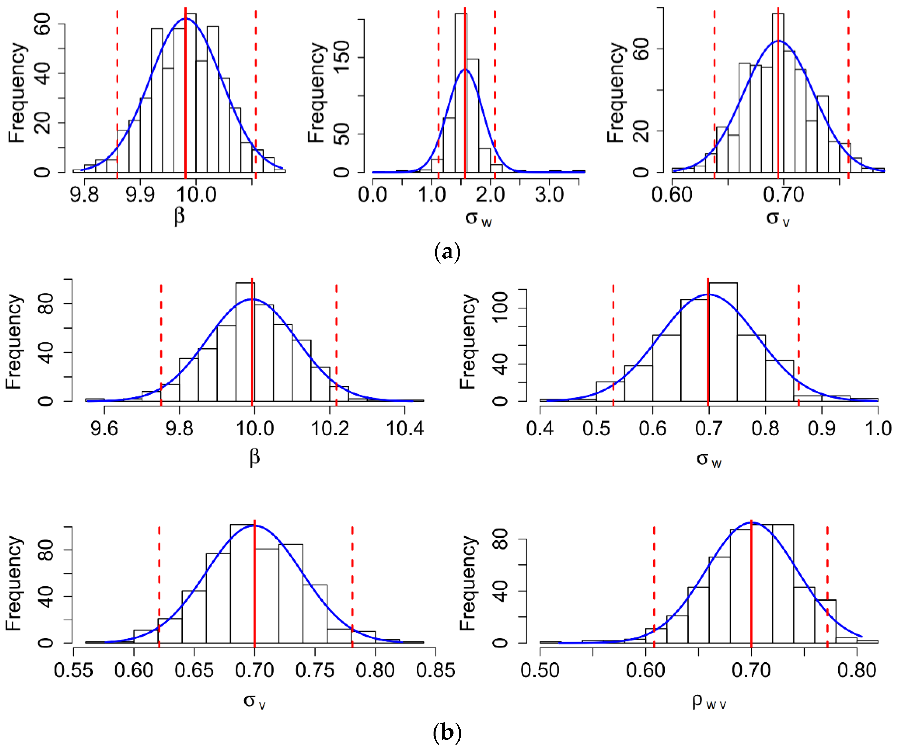
- Set up the values for parameters. To generate a simulated data set, the true parameters of the SFM were fixed as , , and . We chose the Gaussian copula to obtain the correlation between and with the copula parameter set to be .
- Simulate distributions of and . We first simulated the distribution of ( by generating a sequence of 1000 random draws from the Halton sequence. Then, the conditional distribution of given () was simulated by a Gaussian copula using the “BiCopCondSim” function in the software.
- Obtain simulated data of and from their simulated distributions. The inefficiency term was generated by computing the inverse of the half-normal distribution with , given the distribution obtained in the last step; the statistical noise term was computed as the inverse of the normal distribution with , given the distribution . The composite errors were then computed by .
- Simulate data of variables and . The data of the explained variable was generated from uniform random numbers on the interval [0, 1], while the dependent variable was generated according to Equation (29).
3.2. Comparative Study of Two Copula-Based Simultaneous SFMs
- Simulate values of the parameters. The coefficients , , , and were generated from uniformly distributed random numbers on the interval , the standard deviations of inefficiency terms and were generated from uniform random numbers on the interval , and the standard deviations of noise terms and were simulated from uniform random numbers on the interval [0.5, 1]. The dependence between and , and , and and were modeled by Gaussian copulas, where the copula parameters , and were simulated from uniform random numbers on the interval [0.7, 0.95].
- Simulate distributions of and , and and . To simulate the data of and , we first simulated the distribution of () by generating a sequence of 500 random draws from the Halton sequence. Next, we simulated the conditional distribution of given () from a Gaussian copula using the “BiCopCondSim” function in R software, setting up the copula parameter to be . The distributions of () and () were simulated following the same procedure as and , where the copula parameter was set as .
- Generate values for , , , , and . In this step, we generated the values of and , as well as and , given their distributions simulated in the last step. The inefficiency term () was computed by the inverse of the half-normal distribution with a mean of zero and standard deviation of (); the noise term () was computed by the inverse of the normal distribution with a mean of zero and standard deviation of (); and the composite errors were computed by and .
- Generate values for variables and , and and . The explained variables and were simulated as uniform random numbers on the interval , while the dependent variables and were calculated according to Equations (30) and (31), respectively.
3.3. Brief Summary
4. An Application to the Chinese Banking Industry
4.1. Model and Data
4.2. Estimation Results
4.3. Various Measures of Interests
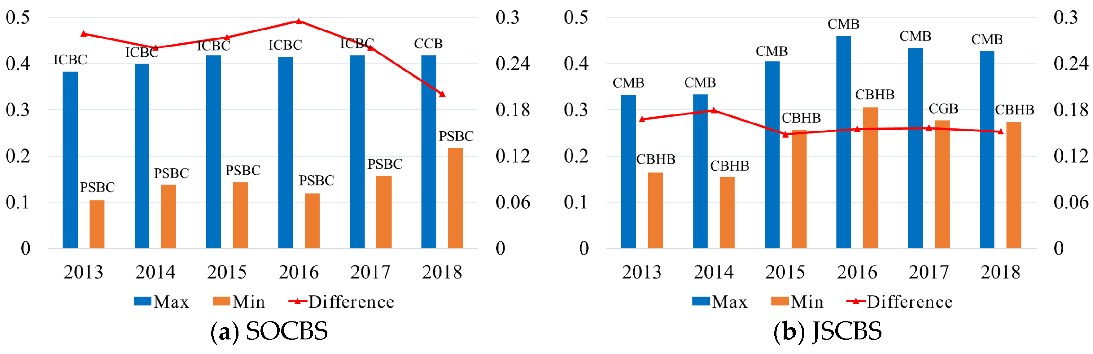
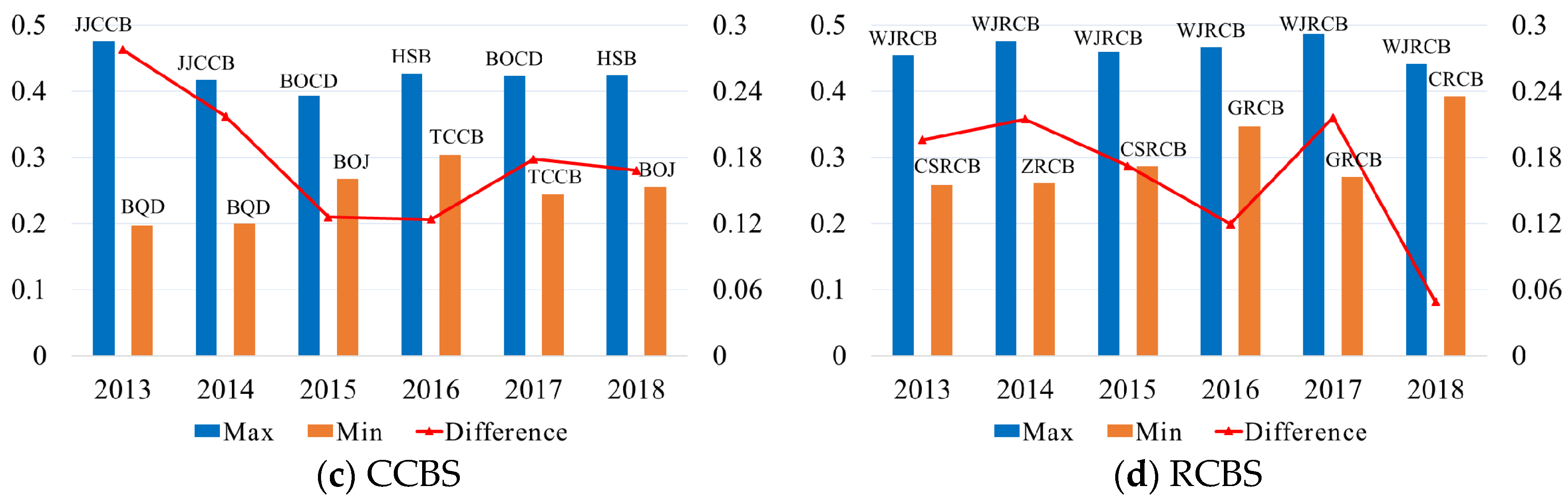
4.3.1. The Lerner Index (LI) and Scale Economies (SC)
4.3.2. Cost Efficiency (CE), Technology Gap Ratio (TGR), and Meta-Frontier Cost Efficiency (MCE)
4.3.3. Brief Summaries
5. Conclusions
Author Contributions
Funding
Acknowledgments
Conflicts of Interest
References
- Fang, J.; Lau, C.-K.M.; Lu, Z.; Tan, Y.; Zhang, H. Bank performance in China: A perspective from bank efficiency, risk-taking and market competition. Pac. Basin Financ. J. 2019, 56, 290–309. [Google Scholar] [CrossRef]
- Bos, J.W.; Kolari, J.W.; Van Lamoen, R.C. Competition and innovation: Evidence from financial services. J. Bank. Financ. 2013, 37, 1590–1601. [Google Scholar] [CrossRef] [Green Version]
- Riaz, M. In competency aspects of microfinance industry: Via SFA approach. J. Econ. Behav. Stud. 2015, 7, 1–12. [Google Scholar] [CrossRef]
- Bos, J.W.; Millone, M. Practice what you preach: Microfinance business models and operational efficiency. World Dev. 2015, 70, 28–42. [Google Scholar] [CrossRef] [Green Version]
- Benedetti, I.; Branca, G.; Zucaro, R. Evaluating input use efficiency in agriculture through a stochastic frontier production: An application on a case study in Apulia (Italy). J. Clean. Prod. 2019, 236, 117609. [Google Scholar] [CrossRef]
- Anik, A.R.; Salam, M.A. Assessing and explaining vegetable growers’ efficiency in the south-eastern hilly districts of Bangladesh. J. Asia Pac. Econ. 2017, 22, 680–695. [Google Scholar] [CrossRef]
- Wang, P.; Deng, X.; Zhang, N.; Zhang, X. Energy efficiency and technology gap of enterprises in Guangdong province: A meta-frontier directional distance function analysis. J. Clean. Prod. 2019, 212, 1446–1453. [Google Scholar] [CrossRef]
- Sun, J.; Du, T.; Sun, W.; Na, H.; He, J.; Qiu, Z.; Yuan, Y.; Li, Y. An evaluation of greenhouse gas emission efficiency in China’s industry based on SFA. Sci. Total Environ. 2019, 690, 1190–1202. [Google Scholar] [CrossRef]
- Lai, H.-P.; Huang, C.J. Maximum likelihood estimation of seemingly unrelated stochastic frontier regressions. J. Product. Anal. 2013, 40, 1–14. [Google Scholar] [CrossRef]
- Fernández, C.; Koop, G.; Steel, M. A Bayesian analysis of multiple-output production frontiers. J. Econom. 2000, 98, 47–79. [Google Scholar] [CrossRef]
- Ferreira, J.T.; Steel, M.F. Model comparison of coordinate-free multivariate skewed distributions with an application to stochastic frontiers. J. Econom. 2007, 137, 641–673. [Google Scholar] [CrossRef]
- Carta, A.; Steel, M.F. Modelling multi-output stochastic frontiers using copulas. Comput. Stat. Data Anal. 2012, 56, 3757–3773. [Google Scholar] [CrossRef] [Green Version]
- Huang, T.-H.; Chiang, D.-L.; Chao, S.-W. A new approach to jointly estimating the Lerner index and cost efficiency for multi-output banks under a stochastic meta-frontier framework. Q. Rev. Econ. Financ. 2017, 65, 212–226. [Google Scholar] [CrossRef]
- Huang, T.-H.; Hu, C.-N.; Chang, B.-G. Competition, efficiency, and innovation in Taiwan’s banking industry—An application of copula methods. Q. Rev. Econ. Financ. 2018, 67, 362–375. [Google Scholar] [CrossRef]
- Bandyopadhyay, D.; Das, A. On measures of technical inefficiency and production uncertainty in stochastic frontier production model with correlated error components. J. Product. Anal. 2006, 26, 165–180. [Google Scholar] [CrossRef]
- Smith, M.D. Stochastic frontier models with dependent error components. Econom. J. 2008, 11, 172–192. [Google Scholar] [CrossRef]
- El Mehdi, R.; Hafner, C.M. Inference in stochastic frontier analysis with dependent error terms. Math. Comput. Simul. 2014, 102, 104–116. [Google Scholar] [CrossRef]
- Wiboonpongse, A.; Liu, J.; Sriboonchitta, S.; Denoeux, T. Modeling dependence between error components of the stochastic frontier model using copula: Application to intercrop coffee production in Northern Thailand. Int. J. Approx. Reason. 2015, 65, 34–44. [Google Scholar] [CrossRef]
- Sriboonchitta, S.; Liu, J.; Wiboonpongse, A.; Denoeux, T. A double-copula stochastic frontier model with dependent error components and correction for sample selection. Int. J. Approx. Reason. 2017, 80, 174–184. [Google Scholar] [CrossRef] [Green Version]
- Lin, H.L.; Tsao, C.C.; Yang, C.H. Bank reforms, competition and efficiency in China’s banking system: Are small city bank entrants more efficient? China World Econ. 2009, 17, 69–87. [Google Scholar] [CrossRef]
- Fungáčová, Z.; Pessarossi, P.; Weill, L. Is bank competition detrimental to efficiency? Evidence from China. China Econ. Rev. 2013, 27, 121–134. [Google Scholar] [CrossRef] [Green Version]
- Hsiao, C.; Yan, S.; Wenlong, B. Evaluating the effectiveness of China’s financial reform—The efficiency of China’s domestic banks. China Econ. Rev. 2015, 35, 70–82. [Google Scholar] [CrossRef] [Green Version]
- Hou, X.; Wang, Q.; Zhang, Q. Market structure, risk taking, and the efficiency of Chinese commercial banks. Emerg. Mark. Rev. 2014, 20, 75–88. [Google Scholar] [CrossRef]
- Zhu, N.; Wu, Y.; Wang, B.; Yu, Z. Risk preference and efficiency in Chinese banking. China Econ. Rev. 2019, 53, 324–341. [Google Scholar] [CrossRef]
- Berger, A.N.; Hasan, I.; Zhou, M. Bank ownership and efficiency in China: What will happen in the world’s largest nation? J. Bank. Financ. 2009, 33, 113–130. [Google Scholar] [CrossRef]
- Chen, Z.; Matousek, R.; Wanke, P. Chinese bank efficiency during the global financial crisis: A combined approach using satisficing DEA and Support Vector Machines. North Am. J. Econ. Financ. 2018, 43, 71–86. [Google Scholar] [CrossRef]
- Fungáčová, Z.; Klein, P.-O.; Weill, L. Persistent and transient inefficiency: Explaining the low efficiency of Chinese big banks. China Econ. Rev. 2020, 59, 101368. [Google Scholar] [CrossRef]
- Chen, X.; Skully, M.; Brown, K. Banking efficiency in China: Application of DEA to pre- and post-deregulation eras: 1993–2000. China Econ. Rev. 2005, 16, 229–245. [Google Scholar] [CrossRef]
- Wang, K.; Huang, W.; Wu, J.; Liu, Y.-N. Efficiency measures of the Chinese commercial banking system using an additive two-stage DEA. Omega 2014, 44, 5–20. [Google Scholar] [CrossRef]
- Jiang, H.; He, Y. Applying data envelopment analysis in measuring the efficiency of Chinese listed banks in the context of macroprudential framework. Mathematics 2018, 6, 184. [Google Scholar] [CrossRef] [Green Version]
- Yin, H.; Yang, J.; Mehran, J. An empirical study of bank efficiency in China after WTO accession. Glob. Financ. J. 2013, 24, 153–170. [Google Scholar] [CrossRef]
- Silva, T.C.; Tabak, B.M.; Cajueiro, D.O.; Dias, M.V.B. A comparison of DEA and SFA using micro-and macro-level perspectives: Efficiency of Chinese local banks. Phys. A: Stat. Mech. Appl. 2017, 469, 216–223. [Google Scholar] [CrossRef]
- Huang, T.-H.; Lin, C.-I.; Chen, K.-C. Evaluating efficiencies of Chinese commercial banks in the context of stochastic multistage technologies. Pac. Basin Financ. J. 2017, 41, 93–110. [Google Scholar] [CrossRef]
- Liu, J.; Wang, M.; Sriboonchitta, S. Examining the Interdependence between the Exchange Rates of China and ASEAN Countries: A Canonical Vine Copula Approach. Sustainability 2019, 11, 5487. [Google Scholar] [CrossRef] [Green Version]
- Shan, Q.; Wongyang, T.; Wang, T.; Tasena, S. A measure of mutual complete dependence in discrete variables through subcopula. Int. J. Approx. Reason. 2015, 65, 11–23. [Google Scholar] [CrossRef]
- Kreinovich, V.; Nguyen, H.T.; Sriboonchitta, S.; Kosheleva, O. Why copulas have been successful in many practical applications: A theoretical explanation based on computational efficiency. In International Symposium on Integrated Uncertainty in Knowledge Modelling and Decision Making; Springer: Cham, Switzerland, 2015; pp. 112–125. [Google Scholar]
- Trivedi, P.; Zimmer, D. A note on identification of bivariate copulas for discrete count data. Econometrics 2017, 5, 10. [Google Scholar] [CrossRef] [Green Version]
- Wei, Z.; Kim, D. On multivariate asymmetric dependence using multivariate skew-normal copula-based regression. Int. J. Approx. Reason. 2018, 92, 376–391. [Google Scholar] [CrossRef]
- Zhu, X.; Wang, T.; Zhang, X.; Wang, L. Comparisons on Measures of Asymmetric Associations. In Proceedings of International Econometric Conference of Vietnam; Springer: Cham, Switzerland, 2019; pp. 185–197. [Google Scholar]
- Wu, C.-C.; Chung, H.; Chang, Y.-H. The economic value of co-movement between oil price and exchange rate using copula-based GARCH models. Energy Econ. 2012, 34, 270–282. [Google Scholar] [CrossRef]
- Sriboonchitta, S.; Nguyen, H.T.; Wiboonpongse, A.; Liu, J. Modeling volatility and dependency of agricultural price and production indices of Thailand: Static versus time-varying copulas. Int. J. Approx. Reason. 2013, 54, 793–808. [Google Scholar] [CrossRef]
- Wei, Z.; Kim, S.; Choi, B.; Kim, D. Multivariate Skew Normal Copula for Asymmetric Dependence: Estimation and Application. Int. J. Inf. Technol. Decis. Mak. 2019, 18, 365–387. [Google Scholar] [CrossRef]
- Fall, F.; Akim, A.-M.; Wassongma, H. DEA and SFA research on the efficiency of microfinance institutions: A meta-analysis. World Dev. 2018, 107, 176–188. [Google Scholar] [CrossRef] [Green Version]
- Coelli, T.J. A Guide to Frontier Version 4.1: A Computer Program for Stochastic Frontier Production and Cost Function Estimation; CEPA Working Papers; University of New England: Armidale, Australia, 1996. [Google Scholar]
- Morris, T.P.; White, I.R.; Crowther, M.J. Using simulation studies to evaluate statistical methods. Stat. Med. 2019, 38, 2074–2102. [Google Scholar] [CrossRef] [PubMed] [Green Version]
- Greene, W. A stochastic frontier model with correction for sample selection. J. Product. Anal. 2010, 34, 15–24. [Google Scholar] [CrossRef] [Green Version]
- Shamshur, A.; Weill, L. Does bank efficiency influence the cost of credit? J. Bank. Financ. 2019, 105, 62–73. [Google Scholar] [CrossRef] [Green Version]
- Spierdijka, L.; Zaourasa, M. Measuring banks’ market power in the presence of economies of scale: A scale-corrected Lerner index. J. Bank. Financ. 2018, 87, 40–48. [Google Scholar] [CrossRef]
- Tan, Y. The impacts of risk and competition on bank profitability in China. J. Int. Financ. Mark. Inst. Money 2016, 40, 85–110. [Google Scholar] [CrossRef] [Green Version]
- Druska, V.; Horrace, W.C. Generalized moments estimation for spatial panel data: Indonesian rice farming. Am. J. Agric. Econ. 2004, 86, 185–198. [Google Scholar] [CrossRef]
- Berger, A.N.; Humphrey, D.B. Bank Scale Economies, Mergers, Concentration, and Efficiency: The US Experience; Working Papers 94-25; Wharton School Center for Financial Institutions, University of Pennsylvania: Philadelphia, PA, USA, 1994. [Google Scholar]
- Barros, C.P.; Ferreira, C.; Williams, J. Analysing the determinants of performance of best and worst European banks: A mixed logit approach. J. Bank. Financ. 2007, 31, 2189–2203. [Google Scholar] [CrossRef]
- Athanasoglou, P.P.; Brissimis, S.N.; Delis, M. Bank-specific, industry-specific and macroeconomic determinants of bank profitability. J. Int. Financ. Mark. Inst. Money 2008, 18, 121–136. [Google Scholar] [CrossRef] [Green Version]
- Lee, C.-C.; Huang, T.-H. Cost efficiency and technological gap in Western European banks: A stochastic metafrontier analysis. Int. Rev. Econ. Financ. 2017, 48, 161–178. [Google Scholar] [CrossRef]
- Wang, Y.; Wang, W.; Wang, J. Credit risk management framework for rural commercial banks in China. J. Financ. Risk Manag. 2017, 6, 48. [Google Scholar] [CrossRef] [Green Version]
- Lee, C.C.; Huang, T.H. What causes the efficiency and the technology gap under different ownership structures in the Chinese banking industry? Contemp. Econ. Policy 2019, 37, 332–348. [Google Scholar] [CrossRef]


| Para | True | Mean | Max | Min | Median | 95% CI | MAE | MAPE |
|---|---|---|---|---|---|---|---|---|
| Conventional SFM | ||||||||
| 10.0 | 9.981 | 10.154 | 9.794 | 9.983 | [9.859, 10.107] | 0.054 | 0.005 | |
| 0.7 | 1.566 | 3.587 | 0.003 | 1.563 | [1.118, 2.074] | 0.870 | 1.243 | |
| 0.7 | 0.695 | 0.790 | 0.602 | 0.695 | [0.638, 0.758] | 0.025 | 0.036 | |
| AIC | 565.1 | 616.5 | 507.8 | 565.2 | [530.8, 600.0] | |||
| BIC | 575.0 | 626.4 | 517.7 | 575.1 | [540.7, 609.9] | |||
| Overall | 0.316 | 0.428 | ||||||
| Copula-based SFM | ||||||||
| 10.0 | 9.993 | 10.420 | 9.556 | 9.996 | [9.751, 10.218] | 0.093 | 0.009 | |
| 0.7 | 0.698 | 0.997 | 0.413 | 0.703 | [0.530, 0.859] | 0.068 | 0.097 | |
| 0.7 | 0.700 | 0.822 | 0.577 | 0.699 | [0.621, 0.781] | 0.031 | 0.045 | |
| 0.7 | 0.700 | 0.804 | 0.518 | 0.703 | [0.608, 0.772] | 0.034 | 0.049 | |
| AIC | 432.4 | 494.5 | 354.0 | 434.0 | [391.9, 470.6] | |||
| BIC | 445.6 | 507.6 | 367.2 | 447.2 | [405.1, 483.8] | |||
| Overall | 0.057 | 0.050 | ||||||
| Criteria | Mean | Max | Min | Median | 95% CI |
|---|---|---|---|---|---|
| Simultaneous SFM with dependent error components | |||||
| AIC | 3031.3 | 3534.4 | 2273.7 | 3035.5 | [2491.4, 3504.1] |
| BIC | 3077.7 | 3580.8 | 2320.1 | 3081.9 | [2537.8, 3550.4] |
| Simultaneous SFM with dependent composite errors | |||||
| AIC | 3259.5 | 4170.1 | 2279.5 | 3275.6 | [2520.8, 4046.0] |
| BIC | 3297.4 | 4208.0 | 2317.4 | 3313.5 | [2558.7, 4083.9] |
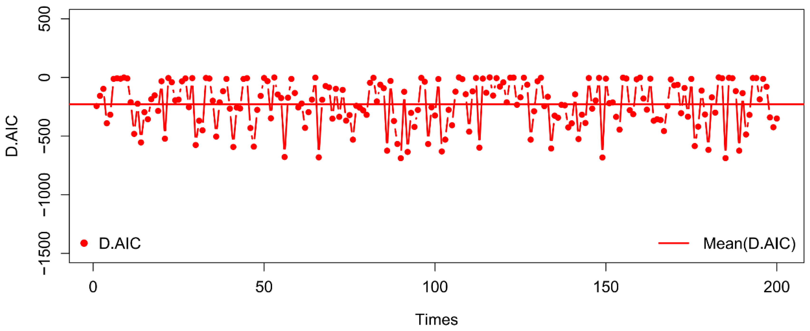
| D.AIC | −228.2 | 0.662 | −688.8 | −207.8 | [−636.0, −1.405] |
| D.BIC | −219.7 | 9.091 | −680.4 | −199.4 | [−627.6, 7.024] |
| Variables | Entire Sample | SOCBs | JSCBs | CCBs | RCBs |
|---|---|---|---|---|---|
| Total revenues () | 1.7778 × 10⁸ (2.5983 × 10⁸) | 6.7775 × 10⁸ (2.6755 × 10⁸) | 1.9337 × 10⁸ (9.0484 × 10⁷) | 3.2843 × 10⁷ (2.5205 × 10⁷) | 1.4155 × 10⁷ (1.3939 × 10⁷) |
| Total assets () | 3.8862 × 10⁹ (6.0574 × 10⁹) | 1.5698 × 10¹⁰ (6.5007 × 10¹⁰) | 3.7259 × 10⁹ (1.8339 × 10⁹) | 7.0699 × 10⁸ (5.6708 × 10⁸) | 2.8958 × 10⁸ (2.9301 × 10⁸) |
| Total costs () | 1.0856 × 10⁸ (1.4852 × 10⁸) | 4.0271 × 10⁸ (1.2239 × 10⁸) | 1.2199 × 10⁸ (5.2576 × 10⁷) | 2.1694 × 10⁷ (1.6508 × 10⁷) | 9.1620 × 10⁶ (8.9081 × 10⁶) |
| Price of labor () | 345.269 (84.186) | 246.245 (38.131) | 397.954 (73.877) | 347.937 (77.403) | 349.817 (63.075) |
| Price of capital () | 1.049 (0.743) | 0.807 (0.738) | 1.254 (0.597) | 1.083 (0.875) | 0.865 (0.477) |
| Price of funds () | 0.027 (0.006) | 0.019 (0.004) | 0.028 (0.005) | 0.029 (0.005) | 0.0262 (0.005) |
| Output price () | 0.049 (0.006) | 0.044 (0.005) | 0.053 (0.005) | 0.048 (0.005) | 0.050 (0.006) |
| No. of bank | 37 | 6 | 10 | 15 | 6 |
| Obs. | 222 | 36 | 60 | 90 | 36 |
| Models | SSFMDEC | SSFMDCE | Single-Equation SFM | |||
|---|---|---|---|---|---|---|
| Variables | Parameter | S.E. | Parameter | S.E. | Parameter | S.E. |
| Constant | 13.123 *** | 0.0050 | 9.8454 *** | 0.0060 | 11.707 ** | 5.1775 |
| 0.2512 *** | 0.0002 | 0.3806 *** | 0.0003 | 0.1712 | 0.2022 | |
| 0.0344 *** | 0.0000 | 0.0494 *** | 0.0004 | 0.0522 *** | 0.0049 | |
| 0.5719 *** | 0.0009 | −0.5109 *** | 0.0010 | −0.5108 | 0.4778 | |
| 1.8974 *** | 0.0005 | 2.1181 *** | 0.0006 | 2.0425 * | 1.0721 | |
| 0.1526 *** | 0.0003 | 0.1205 *** | 0.0003 | 0.1177 *** | 0.0276 | |
| 0.1005 *** | 0.0001 | 0.2423 *** | 0.0001 | 0.1981 | 0.1416 | |
| −0.0483 *** | 0.0002 | −0.1786 *** | 0.0055 | −0.1716 * | 0.0881 | |
| 0.0057 *** | <0.0001 | 0.0220 *** | <0.0001 | 0.0224 ** | 0.0072 | |
| −0.0101 *** | <0.0001 | 0.0264 *** | <0.0001 | 0.0109 | 0.0218 | |
| −0.0921 *** | 0.0184 | −0.2650 *** | 0.0016 | −0.2707 | 0.1729 | |
| 0.0102 ** | 0.0036 | 0.0081 *** | 0.0012 | 0.0083 | 0.0052 | |
| −0.0035 *** | <0.0001 | −0.0002 *** | <0.0001 | −0.0017 | 0.0026 | |
| 0.0219 *** | 0.0002 | 0.0092 *** | 0.0028 | 0.0106 | 0.0080 | |
| −0.0254 *** | 0.0001 | −0.0294 *** | 0.0005 | −0.0340 * | 0.0174 | |
| 0.0110 ** | 0.0043 | |||||
| 0.4587 | 0.4080 | |||||
| 0.0231 | 0.0159 | 0.0915 *** | 0.0242 | |||
| 0.0768 *** | 0.0068 | 0.0716 *** | 0.0103 | |||
| 0.0219 *** | 0.0004 | 0.0162 *** | 0.0008 | |||
| 0.0136 *** | 0.0008 | 0.0012 | 0.0008 | |||
| 0.9800 *** | <0.0001 | |||||
| −28.346 *** | 2.3940 | |||||
| 0.0148 | 0.0736 | 0.1297 | 0.0708 | |||
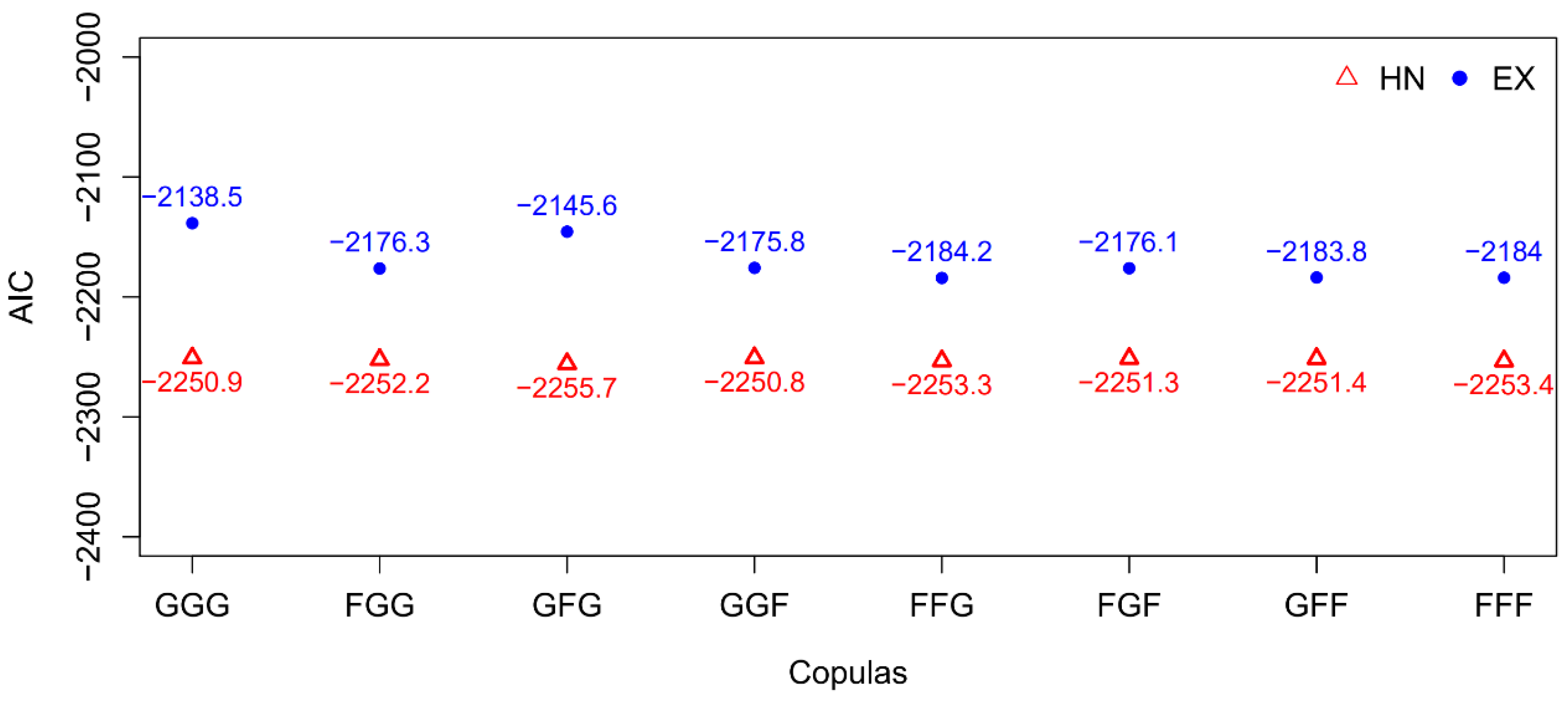
| AIC | −2255.67 | −1907.41 | −413.99 | |||
| Groups | Entire Sample | SOCBs | JSCBs | CCBs | RCBs |
|---|---|---|---|---|---|
| Lerner Index (LI) | |||||
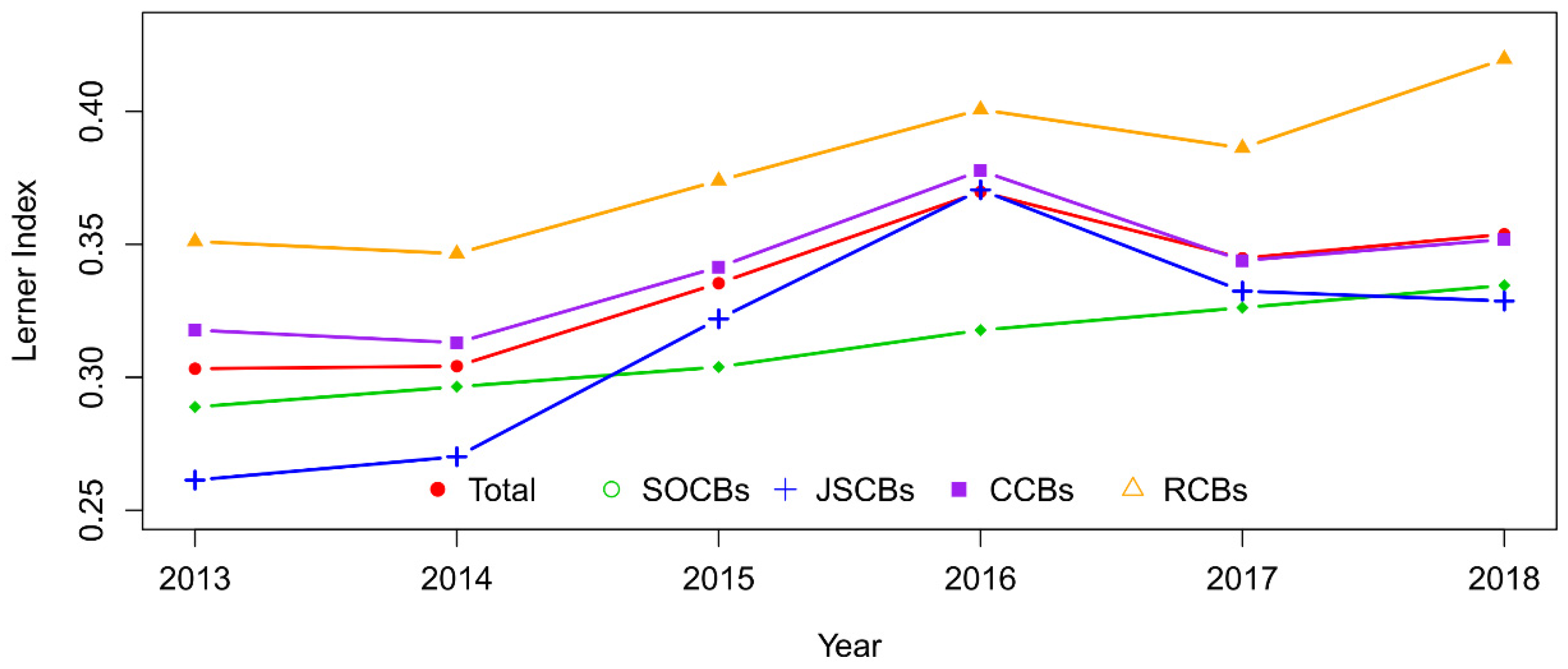
| Mean | 0.335 | 0.311 | 0.314 | 0.341 | 0.380 |
| S.D. | 0.067 | 0.090 | 0.060 | 0.053 | 0.060 |
| Median | 0.337 | 0.327 | 0.318 | 0.339 | 0.392 |
| Min | 0.104 | 0.104 | 0.154 | 0.197 | 0.258 |
| Max | 0.487 | 0.417 | 0.460 | 0.475 | 0.487 |
| Scale Economies (SC) | |||||
| Mean | 1.019 | 1.103 | 1.053 | 0.989 | 0.953 |
| S.D. | 0.056 | 0.015 | 0.021 | 0.025 | 0.033 |
| Median | 1.007 | 1.110 | 1.060 | 0.989 | 0.935 |
| Min | 0.920 | 1.073 | 1.002 | 0.944 | 0.920 |
| Max | 1.121 | 1.121 | 1.077 | 1.038 | 1.003 |
| Obs. | 222 | 36 | 60 | 90 | 36 |
| Groups | Entire Sample | SOCBs | JSCBs | CCBs | RCBs |
|---|---|---|---|---|---|
| Cost Efficiency (CE) | |||||
| Mean | 0.982 | 0.976 | 0.984 | 0.987 | 0.974 |
| S.D. | 0.013 | 0.010 | 0.011 | 0.012 | 0.017 |
| Median | 0.984 | 0.977 | 0.985 | 0.990 | 0.977 |
| Min | 0.945 | 0.961 | 0.960 | 0.947 | 0.945 |
| Max | 1.000 | 0.997 | 0.999 | 1.000 | 0.999 |
| Technology Gap Ratio (TGR) | |||||
| Mean | 0.899 | 0.946 | 0.887 | 0.906 | 0.857 |
| S.D. | 0.069 | 0.028 | 0.073 | 0.065 | 0.072 |
| Median | 0.909 | 0.949 | 0.874 | 0.916 | 0.857 |
| Min | 0.711 | 0.893 | 0.735 | 0.711 | 0.733 |
| Max | 0.999 | 0.995 | 0.999 | 0.998 | 0.998 |
| Meta-frontier Cost Efficiency (MCE) | |||||
| Mean | 0.883 | 0.923 | 0.872 | 0.893 | 0.834 |
| S.D. | 0.063 | 0.023 | 0.065 | 0.059 | 0.061 |
| Median | 0.897 | 0.930 | 0.860 | 0.908 | 0.831 |
| Min | 0.702 | 0.868 | 0.733 | 0.702 | 0.727 |
| Max | 0.981 | 0.964 | 0.980 | 0.981 | 0.979 |
| Obs. | 222 | 36 | 60 | 90 | 36 |
© 2020 by the authors. Licensee MDPI, Basel, Switzerland. This article is an open access article distributed under the terms and conditions of the Creative Commons Attribution (CC BY) license (http://creativecommons.org/licenses/by/4.0/).
Share and Cite
Liu, J.; Wang, M.; Ma, J.; Rahman, S.; Sriboonchitta, S. A Simultaneous Stochastic Frontier Model with Dependent Error Components and Dependent Composite Errors: An Application to Chinese Banking Industry. Mathematics 2020, 8, 238. https://doi.org/10.3390/math8020238
Liu J, Wang M, Ma J, Rahman S, Sriboonchitta S. A Simultaneous Stochastic Frontier Model with Dependent Error Components and Dependent Composite Errors: An Application to Chinese Banking Industry. Mathematics. 2020; 8(2):238. https://doi.org/10.3390/math8020238
Chicago/Turabian StyleLiu, Jianxu, Mengjiao Wang, Ji Ma, Sanzidur Rahman, and Songsak Sriboonchitta. 2020. "A Simultaneous Stochastic Frontier Model with Dependent Error Components and Dependent Composite Errors: An Application to Chinese Banking Industry" Mathematics 8, no. 2: 238. https://doi.org/10.3390/math8020238