Detecting Extreme Values with Order Statistics in Samples from Continuous Distributions


1
Department of Physics and Chemistry, Technical University of Cluj-Napoca, 400641 Cluj-Napoca, Romania
2
Institute of Doctoral Studies, Babeş-Bolyai University, 400091 Cluj-Napoca, Romania
Mathematics 2020, 8(2), 216; https://doi.org/10.3390/math8020216
Submission received: 17 December 2019
/
Revised: 23 January 2020
/
Accepted: 4 February 2020
/
Published: 8 February 2020
(This article belongs to the Special Issue Numerical Methods)
Abstract
:In the subject of statistics for engineering, physics, computer science, chemistry, and earth sciences, one of the sampling challenges is the accuracy, or, in other words, how representative the sample is of the population from which it was drawn. A series of statistics were developed to measure the departure between the population (theoretical) and the sample (observed) distributions. Another connected issue is the presence of extreme values—possible observations that may have been wrongly collected—which do not belong to the population selected for study. By subjecting those two issues to study, we hereby propose a new statistic for assessing the quality of sampling intended to be used for any continuous distribution. Depending on the sample size, the proposed statistic is operational for known distributions (with a known probability density function) and provides the risk of being in error while assuming that a certain sample has been drawn from a population. A strategy for sample analysis, by analyzing the information about quality of the sampling provided by the order statistics in use, is proposed. A case study was conducted assessing the quality of sampling for ten cases, the latter being used to provide a pattern analysis of the statistics.
MSC:
62G30; 62G32; 62H10; 65C60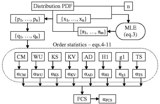
1. Introduction
Under the assumption that a sample of size n, was drawn from a certain population () with a known distribution (with known probability density function, ) but with unknown parameters (in number of m, ), there are alternatives available in order to assess the quality of sampling.
One category of alternatives sees the sample as a whole—and in this case, a series of statistics was developed to measure the agreement between a theoretical (in the population) and observed (of the sample) distribution. This approach is actually a reversed engineering of the sampling distribution, providing a likelihood for observing the sample as drawn from the population. To do this for any continuous distribution, the problem is translated into the probability space by the use of a cumulative distribution function ().
Formally, if takes values on a domain D, then is defined by Equation (1) and defined by Equation (2) is the series of cumulative probabilities associated with the drawings from the sample.
is always a bijective (and invertible; let be its inverse, Equation (3)) function.
The series of cumulative probabilities , independently of the distribution () of the population (X) subjected to the analysis, have a known domain ( for all ) belonging to the continuous uniform distribution (). In the sorted cumulative probabilities ( defined by Equation (4)), sorting defines an order relationship ().
If the order of drawing in sample () and of appearance in the series of associated () is not relevant (e.g., the elements in those sets are indistinguishable), the order relationship defined by Equation (4) makes them () distinguishable (the order being relevant).
A series of order statistics () were developed (to operate on ordered cumulative probabilities ) and they may be used to assess the quality of sampling for the sample taken as a whole (Equations (5)–(10) below): Cramér–von Mises ( in Equation (5), see [1,2]), Watson U2 ( in Equation (6), see [3]), Kolmogorov–Smirnov ( in Equation (7), see [4,5,6]), Kuiper V ( in Equation (8), see [7]), Anderson–Darling ( in Equation (9), see [8,9]), and H1 ( in Equation (10), see [10]).
Recent uses of those statistics include [11] (CM), [12] (WU), [13] (KS), [14] (AD), and [15] (H1). Any of the above given test statistics are to be used, providing a risk of being in error for the assumption (or a likelihood to observe) that the sample () was drawn from the population (X). Usually this risk of being in error is obtained from Monte Carlo simulations (see [16]) applied on the statistic in question and, in some of the fortunate cases, there is also a closed-form expression (or at least, an analytic expression) for of the statistic available as well. In the less fortunate cases, only ‘critical values’ (values of the statistic for certain risks of being in error) for the statistic are available.
The other alternative in assessing the quality of sampling refers to an individual observation in the sample, specifically the less likely one (having associated or with the notations given in Equation (4)). The test statistic is g1 [15], given in Equation (11).
It should be noted that ‘taken as a whole’ refers to the way in which the information contained in the sample is processed in order to provide the outcome. In this scenario (’as a whole’), the entirety of the information contained in the sample is used. As it can be observed in Equations (5)–(10), each formula uses all values of sorted probabilities () associated with the values () contained in the sample, while, as it can be observed in Equation (11), only the extreme value ( or ) is used; therefore, one may say that only an individual observation (the extremum portion of the sample) yields the statistical outcome.
The statistic defined by Equation (11) no longer requires cumulative probabilities to be sorted; one only needs to find the most departed probability from 0.5—see Equation (11)—or, alternatively, to find the smallest (one having associated defined by Equation (4)) and the largest (one having associated defined by Equation (4)), and to find which deviates from 0.5 the most ().
We hereby propose a hybrid alternative, a test statistic (let us call it ) intended to be used in assessing the quality of sampling for the sample, which is mainly based on the less likely observation in the sample, Equation (12).
The aim of this paper is to characterize the newly proposed test statistic () and to analyze its peculiarities. Unlike the test statistics assessing the quality of sampling for the sample taken as a whole (Equations (5)–(10), and like the test statistic assessing the quality of sampling based on the less likely observation of the sample, Equation (11), the proposed statistic, Equation (12), does not require that the values or their associated probabilities () be sorted (as ); since (like the statistic) it uses the extreme value from the sample, one can still consider it a sort of [17]. When dealing with extreme values, the newly proposed statistic, Equation (12), is a much more natural construction of a statistic than the ones previously reported in the literature, Equations (5)–(10), since its value is fed mainly from the extreme value in the sample (see the function in Equation (12)). Later, it will be given a pattern analysis, revealing that it belongs to a distinct group of statistics that are more sensitive to the presence of extreme values. A strategy of using the pool of (Equations (5)–(12)) including in the context of dealing with extreme values is given, and the probability patterns provided by the statistics are analyzed.
The rest of the paper is organized as follows. The general strategy of sampling a CDF from an and the method of combining probabilities from independent tests are given in Section 2, while the analytical formula for the proposed statistic is given in Section 3.1, and computation issues and proof of fact results are given in Section 3.2. Its approximation with other functions is given in Section 3.3. Combining its calculated risk of being in error with the risks from other statistics is given in Section 3.4, while discussion of the results is continued with a cluster analysis in Section 3.5, and in connection with other approaches in Section 3.6. The paper also includes an appendix of the source codes for two programs and accompanying Supplementary Material.
2. Material and Method
2.1. Addressing the Computation of for (s)
A method of constructing the observed distribution of the statistic, Equation (11), has already been reported elsewhere [15]. A method of constructing the observed distribution of the Anderson–Darling () statistic, Equation (9), has already been reported elsewhere [17]; the method for constructing the observed distribution of any via Monte Carlo () simulation, Equations (5)–(12), is described here and it is used for , Equation (12).
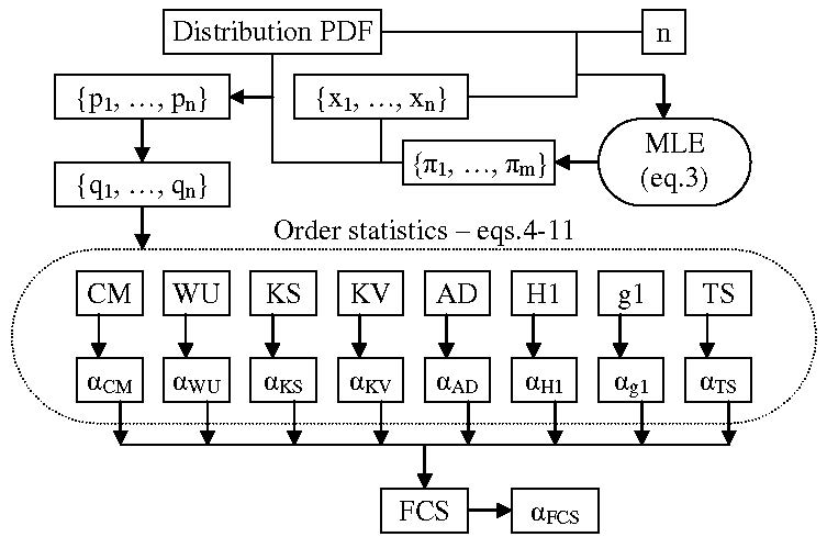
Let us take a sample size of n. The MC simulation needs to generate a large number of samples (let the number of samples be m) drawn from uniform continuous distribution ( in Equation (2)). To ensure a good quality MC simulation, simply using a random number generator is not good enough. The next step (Equations (10)–(12) do not require this) is to sort the probabilities to arrive at from Equation (4) and to calculate an (an order statistic) associated with each sample. Finally, this series of sample statistics ( in Figure 1) must be sorted in order to arrive at the population emulated distribution. Then, a series of evenly spaced points (from 0 to 1000 in Figure 1) corresponding to fixed probabilities (from to in Figure 1) is to be used saving the ( statistic, its observed probability) pairs (Figure 1).
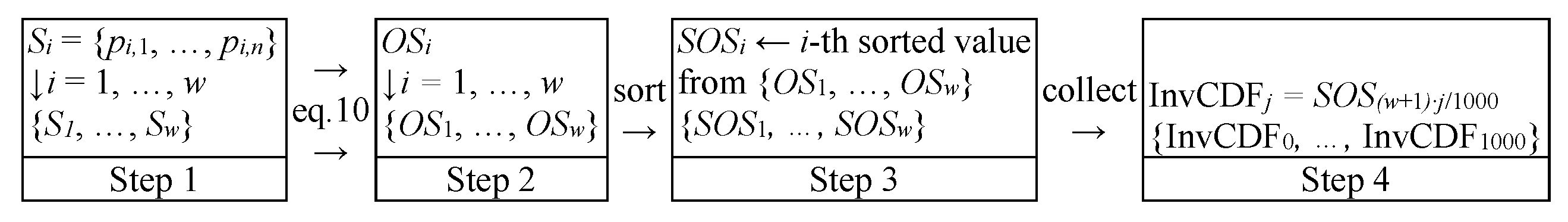
The main idea is how to generate a good pool of random samples from a uniform distribution. Imagine a (pseudo) random number generator, , is available, which generates numbers from a uniform distribution, from a interval; such an engine is available in many types of software and in most cases, it is based on Mersenne Twister [18]. What if we have to extract a sample of size ? If we split in two the interval (then into and ) then for two values (let us say and ), the contingency of the cases is illustrated in Figure 2.
According to the design given in Figure 2, for 4 (=22) drawings of two numbers ( and ) from the [0, 1) interval, a better uniform extraction (, ‘distinguishable’) is (“00”) to extract first () from [0, 0.5) and second () from [0, 0.5), then (“01”) to extract first () from [0, 0.5) and second () from [0.5, 1), then (“10”) to extract first () from [0, 0.5) and second () from [0.5, 1), and finally (“11”) to extract first () from [0.5, 1) and second () from [0.5, 1).
An even better alternative is to do only 3 (=2 + 1) drawings (, ‘undistinguishable’), which is (“0”) to extract both from [0, 0.5), then “1”) to extract one (let us say first) from [0, 0.5), and another (let us say second) from [0.5, 1), and finally, (“2”) to extract both from [0.5, 1) and to keep a record for their occurrences (1, 2, 1), as well. For n numbers (Figure 3), it can be from [0, 0.5) from 0 to n of them, with their occurrences being accounted for.
According to the formula given in Figure 3, for n numbers to be drawn from [0, 1), a multiple of drawings must be made in order to maintain the uniformity of distribution (w from Figure 1 becomes ). In each of those drawings, we actually only pick one of n (random) numbers (from the [0, 1) interval) as independent. In the -th drawing, the first j of them are to be from [0, 0.5), while the rest are to be from [0.5, 1). The algorithm implementing this strategy is given as Algorithm 1.
Algorithm 1 is ready to be used to calculate any (including the first reported here). For each sample drawn from the distribution (the array v in Algorithm 1), the output of it (the array u and its associated frequencies can be modified to produce less information and operations (Algorithm 2). Calculation of the ( output value in Algorithm 2) can be made to any precision, but for storing the result, a data type (4 bytes) is enough (providing seven significant digits as the precision of the observed of the ). Along with a data type (j output value in Algorithm 2) to store each sampled , 5 bytes of memory is required, and the calculation of can be made at a later time, or can be tabulated in a separate array, ready to be used at a later time.
| Algorithm 1: Balancing the drawings from uniform distribution. |
| Input data: n (2 ≤ n, integer) |
| Steps: |
| For i from 1 to n do v[i] ← Rand |
| For j from 0 to n do |
| For i from 1 to j do u[i] ← v[i]/2 |
| For i from j+1 to n do u[i] ← v[i]/2+1/2 |
| occ ← n!/j!/(n-j)! |
| Output u[1],..., u[n], occ |
| EndFor |
| Output data: (n+1) samples (u) of sample size (n) and their occurrences (occ) |
| Algorithm 2: Sampling an order statistic (). |
| Input data: n (2 ≤ n, integer) |
| Steps: |
| For i from 1 to n do v[i] ← Rand |
| For j from 0 to n do |
| For i from 1 to j do u[i] ← v[i]/2 |
| For i from j+1 to n do u[i] ← v[i]/2+1/2 |
| OSj ← any Equations (5)–(12) with p u[1],..., p u[n] |
| Output OSj, j |
| EndFor |
| Output data: (n+1) OS and their occurrences |
As given in Algorithm 2, each use of the algorithm sampling will produce two associated arrays: ( data type) and j ( data type); each of them with values. Running the algorithm times will require bytes for storage of the results and will produce s, ready to be sorted (see Figure 1). With a large amount of internal memory (such as 64 GB when running on a 16/24 cores 64 bit computers), a single process can dynamically address very large arrays and thus can provide a good quality, sampled . To do this, some implementation tricks are needed (see Table 1).
Depending on the value of the sample size (n), the number of repetitions () for sampling of , using Algorithm 2, from runs, is , while the length () of the variable () storing the dynamic array () from Table 1 is . After sorting the s (of , see Table 1; total number of ) another trick is to extract a sample series at evenly spaced probabilities from it (from to in Figure 1). For each pair in the sample ( varying from 0 to = 1000 in Table 1), a value of the is extracted from array (which contains ordered values and frequencies indexed from 0 to 1), while the MC-simulated population size is . A program implementing this strategy is available upon request ().
The associated objective (with any statistic) is to obtain its and thus, by evaluating the for the statistical value obtained from the sample, Equations (5)–(12), to associate a likelihood for the sampling. Please note that only in the lucky cases is it possible to do this; in the general case, only critical values (values corresponding to certain risks of being in error) or approximation formulas are available (see for instance [1,2,3,5,7,8,9]). When a closed form or an approximation formula is assessed against the observed values from an MC simulation (such as the one given in Table 1), a measure of the departure such as the standard error () indicates the degree of agreement between the two. If a series of evenly spaced points ( points indexed from 0 to in Table 1) is used, then a standard error of the agreement for inner points of it (from 1 to , see Equation (13)) is safe to be computed (where stands for the observed probability while for the estimated one).
In the case of , evenly spaced points in the interval in the context of MC simulation (as the one given in Table 1) providing the values of OS statistic in those points (see Figure 1), the observed cumulative probability should (and is) taken as , while is to be (and were) taken from any closed form or approximation formula for the statistic (labeled ) as , where are the values collected by the strategy given in Figure 1 operating on the values provided by Algorithm 2. Before giving a closed form for of (Equation (12)) and proposing approximation formulas, other theoretical considerations are needed.
2.2. Further Theoretical Considerations Required for the Study
When the is known, it does not necessarily imply that its statistical parameters ( in Equations (1)–(3)) are known, and here, a complex problem of estimating the parameters of the population distribution from the sample (it then uses the same information as the one used to assess the quality of sampling) or from something else (and then it does not use the same information as the one used to assess the quality of sampling) can be (re)opened, but this matter is outside the scope of this paper.
The estimation of distribution parameters for the data is, generally, biased by the presence of extreme values in the data, and thus, identifying the outliers along with the estimation of parameters for the distribution is a difficult task operating on two statistical hypotheses. Under this state of facts, the use of a hybrid statistic, such as the proposed one in Equation (12), seems justified. However, since the practical use of the proposed statistics almost always requires estimation of the population parameters (and in the examples given below, as well), a certain perspective on estimation methods is required.
Assuming that the parameters are obtained using the maximum likelihood estimation method (MLE, Equation (14); see [19]), one could say that the uncertainty accompanying this estimation is propagated to the process of detecting the outliers. With a series of statistics ( for Equations (5)–(10) and for Equations (5)–(12)) assessing independently the risk of being in error (let be those risks), assuming that the sample was drawn from the population, the unlikeliness of the event ( in Equation (15) below) can be ascertained safely by using a modified form of Fisher’s “combining probability from independent tests” method (, see [10,20,21]; Equation (15)), where is the of distribution with degrees of freedom.
Two known symmetrical distributions were used (, see Equation (1)) to express the relative deviation from the observed distribution: Gauss ( in Equation (16)) and generalized Gauss–Laplace ( in Equation (17)), where (in both Equations (16) and (17)) .
The distributions given in Equations (16) and (17) will be later used to approximate the of as well as in the case studies of using the order statistics. For a sum ( in Equation (18)) of uniformly distributed () deviates (as in Equation (2)) the literature reports the Irwin–Hall distribution [22,23]. The is:
3. Results and Discussion
3.1. The Analytical Formula of for
The of depends (only) on the sample size (n), e.g., . As the proposed equation, Equation (12), resembles (as an inverse of) a sum of normal deviates, we expected that the will also be connected with the Irwin–Hall distribution, Equation (18). Indeed, the conducted study has shown that the inverse () of the variable (x) following the follows a distribution () of which the is given in Equation (19). Please note that the similarity between Equations (18) and (19) is not totally coincidental; (see Equation (12)) is more or less a sum of uniform distributed deviates divided by the highest one. Also, for any positive arbitrary generated series, its ascending (x) and descending () sorts are complementary. With the proper substitution, can be expressed as a function of —see Equation (20).
Unfortunately, the formulas, Equation (18) to Equation (20), are not appropriate for large n and p ( from Equation (19)), due to the error propagated from a large number of numerical operations (see further Table 2 in Section 3.2). Therefore, for , a similar expression providing the value for is more suitable. It is possible to use a closed analytical formula for as well, Equation (21). Equation (21) resembles the Irwin–Hall distribution even more closely than Equation (20)—see Equation (22).
For consistency in the following notations, one should remember the definition of , see Equation (1), and then we mark the connection between notations in terms of the analytical expressions of the functions, Equation (23):
One should notice (Equation (1); Equation (23)) that the infimum for the domain of (1) is the supremum for the domain of (1) and the supremum (n) for the domain of is the infimum (1/n) for the domain of . Also, has the median () at , while has the median (which is also the mean and mode) at . The distribution of is symmetrical.
For , the is linear (), while for , it is a mixture of two square functions: , for (and ), and for (and ). With the increase of n, the number of mixed polynomials of increasing degree defining its expression increases. Therefore, it has no way to provide an analytical expression for of , not even for certain p values (such as ‘critical’ analytical functions).
The distribution of can be further characterized by its central moments (Mean , Variance , Skewness , and Kurtosis in Equation (24)), which are closely connected with the Irwin–Hall distribution.
3.2. Computations for the of and Its Analytical Formula
Before we proceed in providing the simulation results, some computational issues must be addressed. Any of the formulas provided for of (Equations (19) and (21); or Equations (20) and (22) both connected with Equation (18)), will provide almost exact calculations as long as computations with the formulas are conducted with an engine or package that performs the operations with rational numbers to an infinite precision (such as is available in the Mathematica software [24]), when also the value of y (, of floating point type) is converted to a rounded, rational number. Otherwise, with increasing n, the evaluation of for using either Equation (19) to Equation (22) carries huge computational errors (see the alternating sign of the terms in the sums of Equations (18), (19), and (21)). In order to account for those computational errors (and to reduce their magnitude) an alternate formula for the of is proposed (Algorithm 3), combining the formulas from Equations (19) and (21), and reducing the number of summed terms.
| Algorithm 3: Avoiding computational errors for . |
| Input data: n (n ≥ 2, integer), x (1 ≤ x ≤ 1/n, real number, double precision) |
| ; // Equation (19), Equation (21) |
| if y <(n+1)/2 |
| else if y >(n+1)/2 |
| else |
| Output data: and |
Table 2 contains the sums of the residuals ( in Equation (13), ) of the agreement between the observed of (, for i from 1 to 999) and the calculated of (the values are calculated using Algorithm 3 from for i from 1 to 999) for some values of the sample size (n). To prove the previous given statements, Table 2 provides the square sums of residuals computed using three alternate formulas (from Equation (20) and from Equation (22), along with the ones from Algorithm 3).
As given in Table 2, the computational errors by using either Equation (20) (or Equation (19)) and Equation (22) (or Equation (21)) until n = 34 are reasonably low, while from n = 42, they become significant. As can be seen (red values in Table 2), double precision alone cannot cope with the large number of computations, especially as the terms in the sums are constantly changing their signs (see in Equations (19) and (21)).
The computational errors using Algorithm 3 are reasonably low for the whole domain of the simulated of (with n from 2 to 55), but the combined formula (Algorithm 3) is expected to lose its precision for large n values, and therefore, a solution to safely compute ( for , and ) is to operate with rational numbers.
One other alternative is to use GNU GMP (Multiple Precision Arithmetic Library [25]). The calculations are the same (Algorithm 3); the only difference is the way in which the temporary variables are declared (instead of , the variables become initialized later with a desired precision).
For convenience, the FreePascal [26] implementation for of the Irwin–Hall distribution (Equation (18), called in the context of evaluating the of in Equations (20) and (22)) is given as Algorithm 4.
| Algorithm 4: FreePascal implementation for calculating the of . |
| Input data: n (integer), x (real number, double precision); |
| var k,i: integer; // enough for n < 32,768 |
| var z,y: mpf_t; // or instead of |
| Begin // for Irwin–Hall distribution |
| mpf_set_default_prec(128); //or bigger, 256, 512,... |
| mpf_init(y); mpf_init(z); //y := 0.0; |
| for k := trunc(x) downto 0 do begin //main loop |
| If(k mod 2 = 0) // z := 1.0 or z := −1.0; |
| then mpf_set_si(z,1) //z := 1.0; |
| else mpf_set_si(z,-1); //z := −1.0; |
| for i := n − k downto 1 do z := z*(x − k)/i; |
| for i := k downto 1 do z := z*(x− k)/i; |
| y := y + z; |
| end; |
| pIH_gmp := mpf_get_d(y); mpf_clear(z); mpf_clear(y); |
| End; |
| Output data: p (real number, double precision) |
In Algorithm 4, the changes made to a classical code running without GNU GMP floating point arithmetic functions are written in blue color. For convenience, the combined formula (Algorithm 3) trick for avoiding the computation errors can be implemented with the code given as Algorithm 4 at the call level, Equation (25). If pIH(x:double; n:integer):double returns the value from Algorithm 4, then , as given in Equation (25), safely returns the combined formula (Algorithm 3) with (or without) GNU GMP.
Regarding Table 2, Algorithm 4 listed data, from n = 2 to n = 55, the calculation of the residuals were made with (64 bits), (FreePascal 80 bits), and -128 bits (GNU GMP). The sum of residuals (for all n from 2 to 55) differs from to with less than and the same for with 128 bits, which safely provides confidence in the results provided in Table 2 for the combined formula (last column, Algorithm 4). The deviates for agreement in the calculation of for are statistically characterized by (Equation (13)), , and in Table 3.
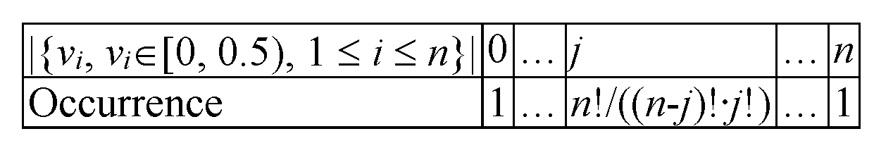
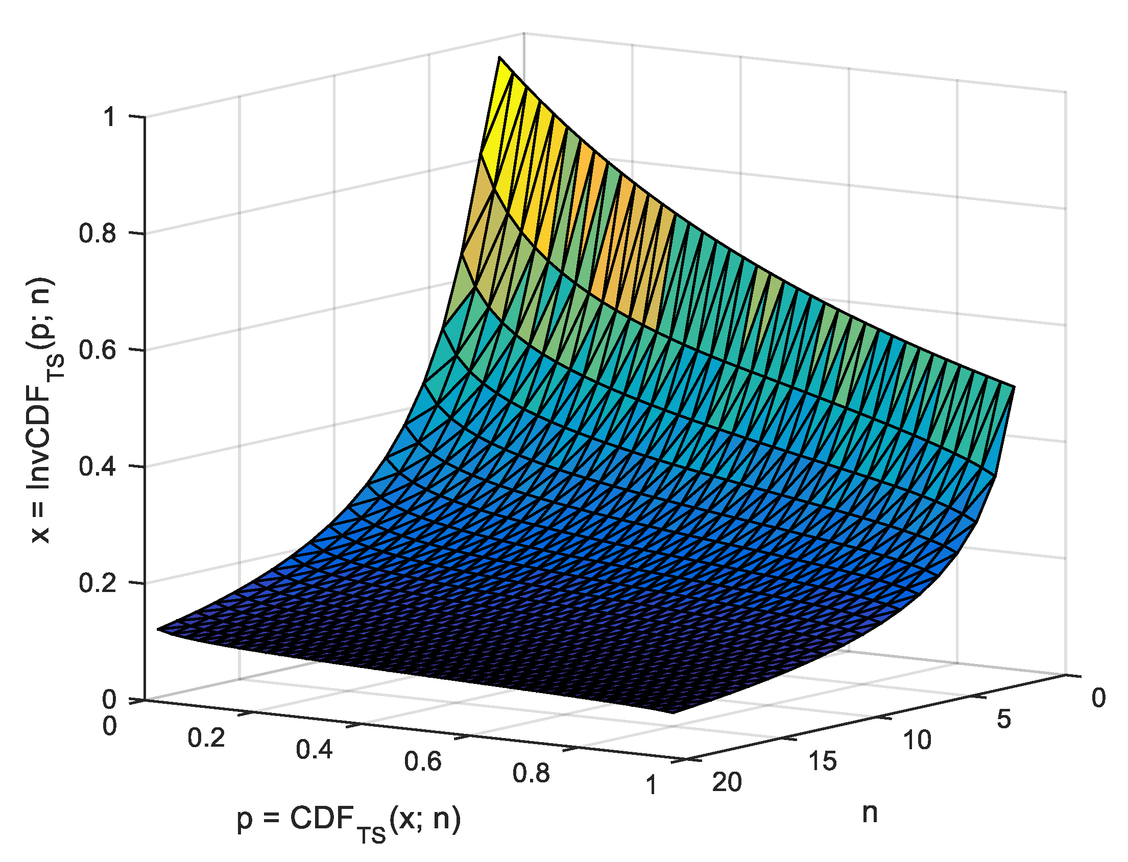
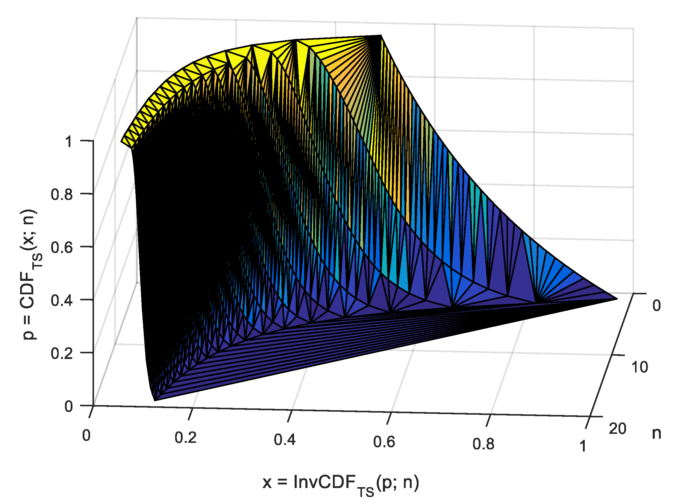
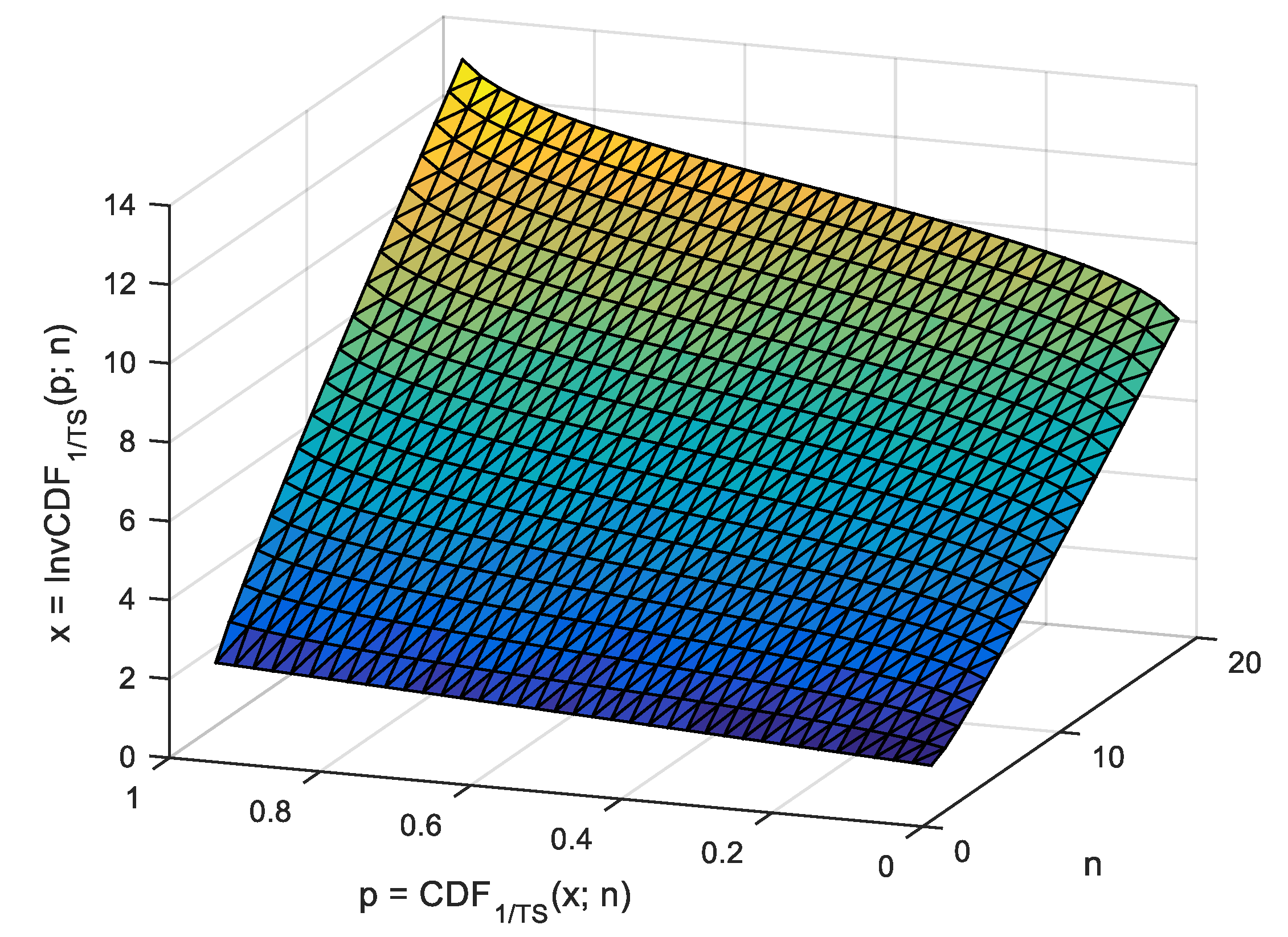
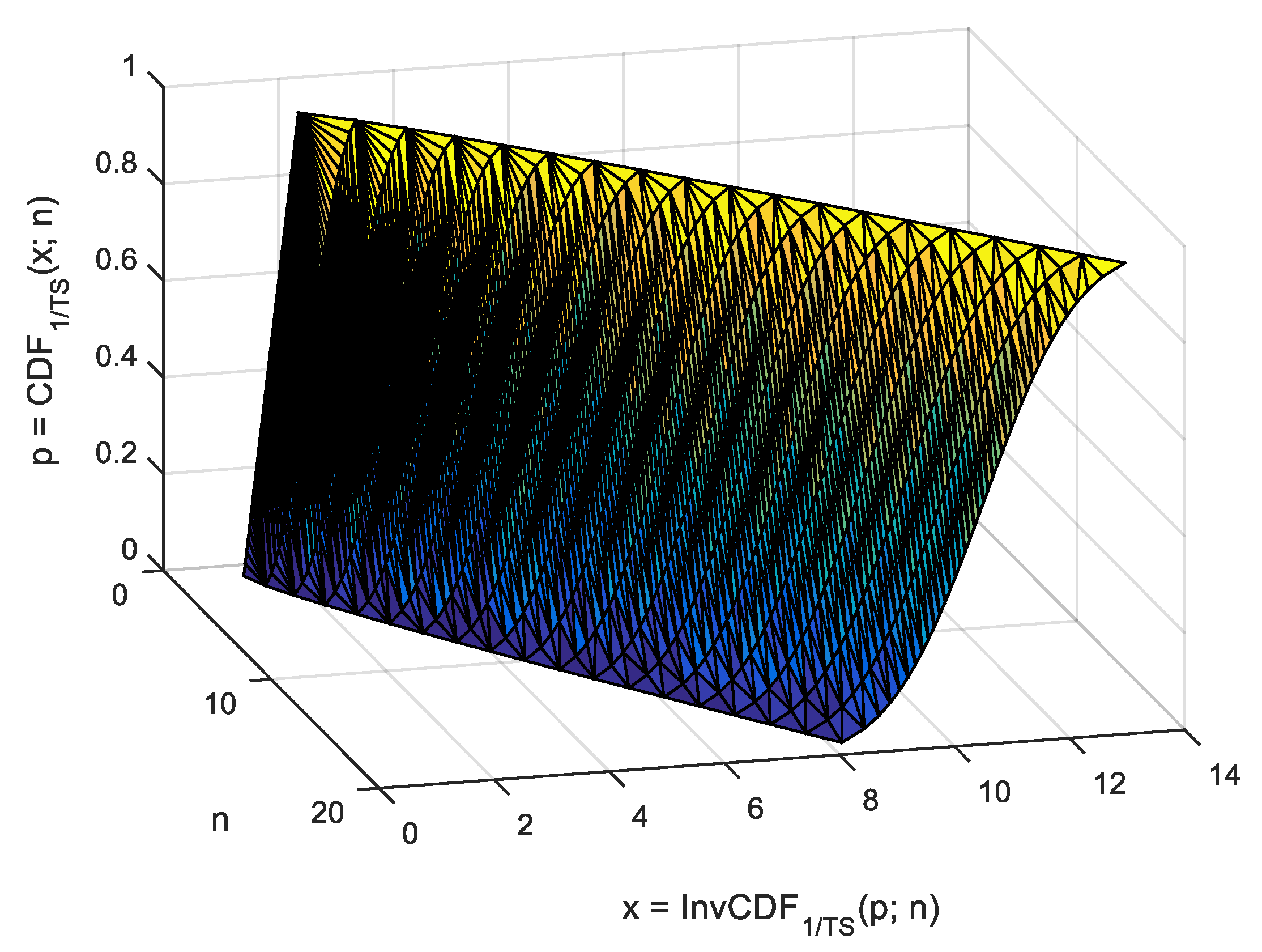
The of agreement (Table 3) between the expected value and the observed one (Algorithm 4, Equation (12), Table 1) of the is safely below the resolution for the grid of observing points ( in Table 1; in Table 3; two orders of magnitude). By using Algorithm 4, Figure 4, Figure 5, Figure 6 and Figure 7 depict the shapes of , , , and for n from 2 to 20.
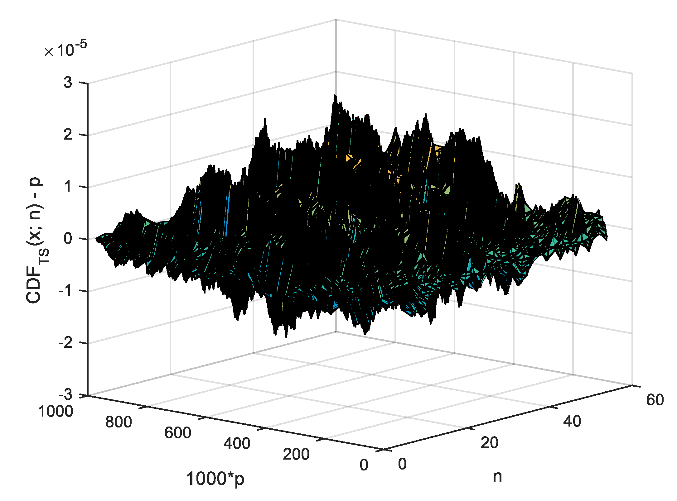
Finally, for the domain of the simulated of the population for n from 2 to 54, the error in the odd points of the grid (for from 1 to 999 with a step of 2) is depicted in Figure 8 (the calculations of theoretical for made with at a precision of at least 256 bits). As can be observed in Figure 8, the difference between p and is rarely larger than and never larger than (the boundary of the representation in Figure 8) for n ranging from 2 to 54.
Based on the provided results, one may say that there is no error in saying that Equations (19) and (21) are complements (see Equation (23) as well) of the of given as Equation (12). As long as the calculations (of either Equations (19) and (21)) are conducted using rational numbers, either formula provides the most accurate result. The remaining concerns are how large those numbers can be (e.g., the range of n). This is limited only by the amount of memory available and how precise the calculations are. This reaches the maximum defined by the measurement of data precision, and finally, the resolutions are provided, which are given by the precision of converting (if necessary) the value given by Equation (12) from float to rational. Either way, some applications prefer approximate formulas, which are easier to calculate, and are considered common knowledge for interpreting the results. For those reasons, the next section describes approximation formulas.
3.3. Approximations of of with Known Functions
Considering, once again, Equation (24), for sufficiently large n, the distribution of is approximately normal (Equation (26). For normal Gauss distribution, see Equation (16)).
Even better (than Equation (26)), for large values of n, a generalized Gauss–Laplace distribution (see Equation (17)) can be used to approximate the statistic. Furthermore, for those looking for critical values of the statistic, the approximation of the statistic to a generalized Gauss–Laplace distribution may provide safe critical values for large n. One way to derive the parameters of the generalized Gauss–Laplace distribution approximating the statistic is by connecting the kurtosis and skewness of the two (Equation (27)).
With and given by Equation (27) and (Equation (24)), the of the generalized Gauss–Laplace distribution (Equation (17)), which approximates (for large n), is given in Equation (28).
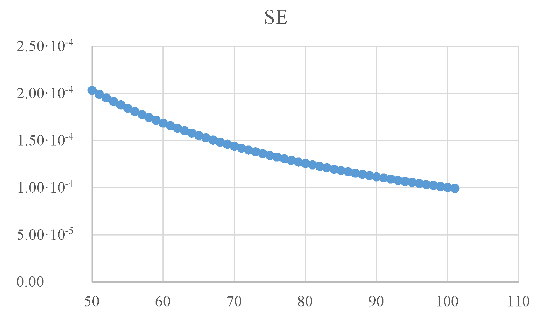
The errors of approximation (with Equation (29)) of (from Algorithm 3) with (from Equations (27) and 28) are depicted in Figure 9 using a grid of 52 × 999 points for and .
As can be observed in Figure 9, the confidence in approximation of with the increases with the sample size (n), but the increase is less than linear. The tendency is to approximately linearly decrease with an exponential increase.
The calculation of for is a little tricky, as anticipated previously (see Section 3.2). To avoid the computation errors in the calculation of , a combined formula is more appropriate (Algorithms 3 and 4). With and , depending on the value of y (, where x is the sample statistic of , Equation (12)), only one (from and p, where ) is suitable for a precise calculation.
An important remark at this point is that is the median, mean, and mode for (see Section 3.1). Indeed, any symbolic calculation with either of the formulas from Equation (19) to Equation (22) will provide that , or, expressed with , .
3.4. The Use of for to Measure the Departure between an Observed Distribution and a Theoretical One
With any of Equations (5)–(12), a likelihood to observe an observed sample can be ascertained. One may ask which statistic is to be trusted. The answer is, at the same time, none and all, as the problem of fitting the data to a certain distribution involves the estimation of the distribution’s parameters—such as using MLE, Equation (14). In this process of estimation, there is an intrinsic variability that cannot be ascertained by one statistic alone. This is the reason that calculating the risk of being in error from a battery of statistics is necessary, Equation (15).
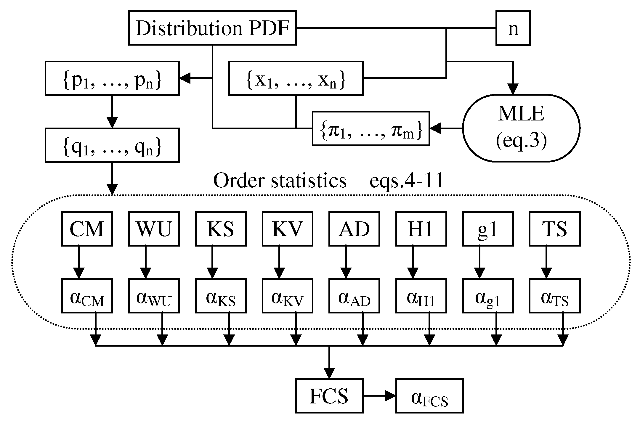
Also, one may say that the statistic (Equation (11)) is not associated with the sample, but to its extreme value(s), while others may say the opposite. Again, the truth is that both are right, as in certain cases, samples containing outliers are considered not appropriate for the analysis [27], and in those cases, there are exactly two modes of action: to reject the sample or to remove the outlier(s). Figure 10 gives the proposed strategy of assessing the samples using order statistics.
As other authors have noted, in nonparametric problems, it is known that order statistics, i.e., the ordered set of values in a random sample from least to greatest, play a fundamental role. ‘A considerable amount of new statistical inference theory can be established from order statistics assuming nothing stronger than continuity of the cumulative distribution function of the population’ as [28] noted, a statement that is perfectly valid today.
In the following case studies, the values of the sample statistics were calculated with Equations (5)–(10) (; see also Figure 10), while the risks of being in error—associated with the values of sample statistics ( for those)—were calculated with the program developed and posted online available at http://l.academicdirect.org/Statistics/tests. The (Equation (11)) and were calculated as given in [15], while the (Equation (12)) was calculated with Algorithm 4. For and , Equation (15) was used.
- Case study 1.
Data: “Example 1” in [29]; Distribution: Gauss (Equation (16)); Sample size: n = 10; Population parameters (MLE, Equation (14)): = 575.2; = 8.256; Order statistics analysis is given in Table 4. Conclusion: at = 5% risk of being in error, the sample does not have an outlier ( = 11.2%) but it is a bad drawing from normal (Gauss) distribution, with less than the imposed level ( = 5%) likelihood to appear from a random draw ( = 4.5%).
- Case study 2.
Data: “Example 3” in [29]; Distribution: Gauss (Equation (16)); Sample size: n = 15; Population parameters (MLE, Equation (14)): = 0.018; = 0.532; Order statistics analysis is given in Table 4. Conclusion: at = 5% risk of being in error, the sample does not have an outlier ( = 10.9%) and it is a good drawing from normal (Gauss) distribution, with more than the imposed level ( = 5%) likelihood to appear from a random draw ( = 59.6%).
- Case study 3.
Data: “Example 4” in [29]; Distribution: Gauss (Equation (16)); Sample size: n = 10; Population parameters (MLE, Equation (14)): = 3.406; = 0.732; Order statistics analysis is given in Table 4. Conclusion: at = 5% risk of being in error, the sample does not have an outlier ( = 45.1%) and it is a good drawing from normal (Gauss) distribution, with more than the imposed level ( = 5%) likelihood to appear from a random draw ( = 79.7%).
- Case study 4.
Data: “Example 5” in [29]; Distribution: Gauss (Equation (16)); Sample size: n = 8; Population parameters (MLE, Equation (14)): = 4715; = 140.8; Order statistics analysis is given in Table 4. Conclusion: at = 5% risk of being in error, the sample does not have an outlier ( = 25.5%) and it is a good drawing from normal (Gauss) distribution, with more than the imposed level ( = 5%) likelihood to appear from a random draw ( = 34.6%).
- Case study 5.
Data: “Table 4” in [15]; Distribution: Gauss (Equation (16)); Sample size: n = 206; Population parameters (MLE, Equation (14)): = 6.481; = 0.829; Order statistics analysis is given in Table 4. Conclusion: at = 5% risk of being in error, the sample have an outlier ( = 3.4%) and it is a good drawing from normal (Gauss) distribution, with more than the imposed level ( = 5%) likelihood to appear from a random draw ( = 66.1%).
- Case study 6.
Data: “Table 1, Column 1” in [30]; Distribution: Gauss (Equation (16)); Sample size: n = 166; Population parameters (MLE, Equation (14)): = −0.348; = 1.8015; Order statistics analysis is given in Table 4. Conclusion: at = 5% risk of being in error, the sample does not have an outlier ( = 24.7%) and it is a good drawing from normal (Gauss) distribution, with more than the imposed level ( = 5%) likelihood to appear from a random draw ( = 68.7%).
- Case study 7.
Data: “Table 1, Set BBB” in [31]; Distribution: Gauss (Equation (16)); Sample size: n = 105; Population parameters (MLE, Equation (14)): = −0.094; = 0.762; Order statistics analysis is given in Table 4. Conclusion: at = 5% risk of being in error, the sample does not have an outlier ( = 72.9%) and it is a good drawing from normal (Gauss) distribution, with more than the imposed level ( = 5%) likelihood to appear from a random draw ( = 18.8%).
- Case study 8.
Data: “Table 1, Set SASCAII” in [31]; Distribution: Gauss (Equation (16)); Sample size: n = 47; Population parameters (MLE, Equation (14)): = 1.749; = 0.505; Order statistics analysis is given in Table 4. Conclusion: at = 5% risk of being in error, the sample does not have an outlier ( = 98.0%) and it is a good drawing from normal (Gauss) distribution, with more than the imposed level ( = 5%) likelihood to appear from a random draw ( = 65.5%).
- Case study 9.
Data: “Table 1, Set TaxoIA” in [31]; Distribution: Gauss (Equation (16)); Sample size: n = 63; Population parameters (MLE, Equation (14)): = 0.744; = 0.670; Order statistics analysis is given in Table 4. Conclusion: at = 5% risk of being in error, the sample does not have an outlier ( = 74.6%) and it is a good drawing from normal (Gauss) distribution, with more than the imposed level ( = 5%) likelihood to appear from a random draw ( = 95.2%).
- Case study 10.
Data: “Table 1, Set ERBAT” in [31]; Distribution: Gauss (Equation (16)); Sample size: n = 25; Population parameters (MLE, Equation (14)): = 0.379; = 1.357; Order statistics analysis is given in Table 4. Conclusion: at = 5% risk of being in error, the sample does not have an outlier ( = 87.9%) and it is a good drawing from normal (Gauss) distribution, with more than the imposed level ( = 5%) likelihood to appear from a random draw ( = 89.5%).
3.5. The Patterns in the Order Statistics
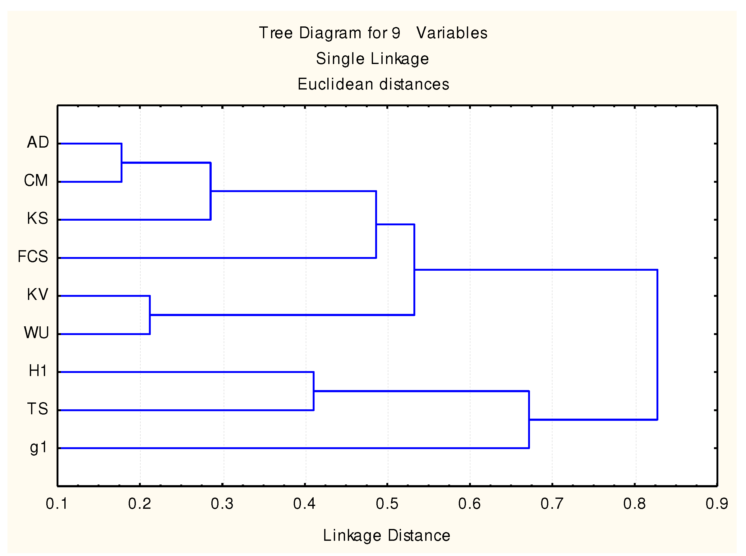
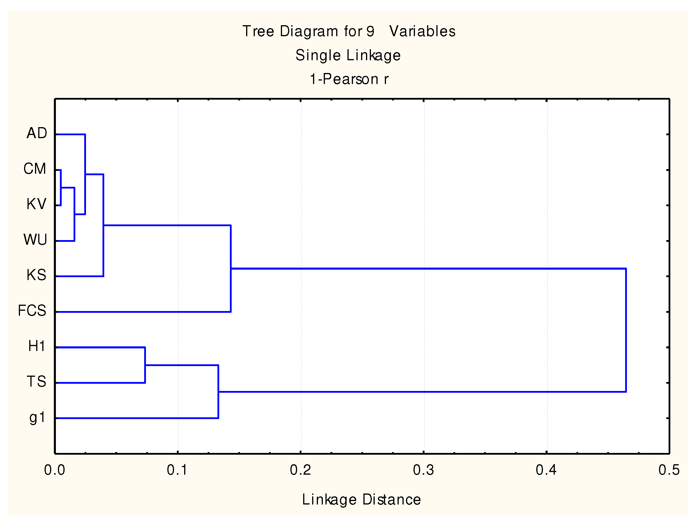
A cluster analysis on the risks of being in error, provided by the series of order statistics on the case studies considered in this study, may reveal a series of peculiarities (Figure 11 and Figure 12). The analysis given here is based on the series of the above given case studies in order to illustrate similarities (and not to provide a ‘gold standard’ as in [32] or in [33]).
Both clustering methods illustrated in Figure 11 and Figure 12 reveal two distinct groups of statistics: {AD, CM, KV, WU, KS} and {H1, TS, g1}. The combined test FCS is also attracted (as expected) to the largest group. When looking at single Euclidean distances (Figure 11) of the largest group, two other associations should be noticed {AD, CM, KS} and {KV, WU}, suggesting that those groups carry similar information, but when looking at the Pearson disagreements (Figure 12), we must notice that the subgroups are changed {CM, KV, WU}, {AD}, and {KS}, with no hint of an association with their calculation formulas (Equations (5)–(9)); therefore, their independence should not be dismissed. The second group {H1, TS, g1} is more stable, maintaining the same clustering pattern of the group ({H1, TS}, {g1} in Figure 12).
Taking into account that the g1 test (Equation (11)) was specifically designed to account for outliers suggests that the H1 and TS tests are more sensitive to the outliers than other statistics, and therefore, when the outliers (or just the presence of extreme values) are the main concern in the sampling, it is strongly suggested to use those tests. The H1 statistic is a Shannon entropy formula applied in the probability space of the sample. When accounting for this aspect in the reasoning, the rassociation of the H1 with TS suggests that TS is a sort of entropic measure (max-entropy, to be more exact [34], a limit case of generalized Rényi’s entropy [35]). Again, the g1 statistic is alone in this entropic group, suggesting that it carries a unique fingerprint about the sample—specifically, about its extreme value (see Equation (11))—while the others account for the context (the rest of the sampled values, Equations (10) and (12)).
Regarding the newly proposed statistic (TS), from the given case studies, the fact that it belongs to the {H1, TS, g1} group strongly suggests that it is more susceptible to the presence of outliers (such as g1, purely defined for this task, and unlike the well known statistics defined by Equations (5)–(9)).
Moreover, one may ask that, if based on the risks being in error provided by the statistics from case studies 1 to 10, some peculiarity about TS or another statistic involved in this study could be revealed. An alternative is to ask if the values of risks can be considered to be belonging to the same population or not, and for this, the K-sample Anderson–Darling test can be invoked [36]. With the series of probabilities, there are actually tests to be conducted (for each subgroup of 2, 3, 4, 5, 6, 7, 8, and 9 statistics picked from nine possible choices) and for each of them, the answer is same: At the 5% risk of being in error, it cannot be rejected that the groups (of statistics) were selected from identical populations (of statistics), so, overall, any of those statistics perform the same.
3.6. Another Rank Order Statics Method and Other Approaches
The series of rank order statistics included in this study, Equations (5)–(11), covers the most known rank order statistics reported to date. However, when considering a new order statistic not included there, the use of it in the context of combining methods, Equation (15), only increases the degrees of freedom , while the design of using (Figure 10) is changed accordingly.
It should be noted that the proposed approach is intended to be used for small sample sizes, when no statistic alone is capable of high precision and high trueness. With the increasing sample size, all statistics should converge to the same risk of being in error and present other alternatives, such as the superstatistical approach [40]. In the same context, each of the drawings included in the sample are supposed to be independent. In the presence of correlated data (such as correlated in time), again, other approaches, such as the one communicated in [41], are more suited.
4. Conclusions
A new test statistic to be used to measure the agreement between continuous theoretical distributions and samples drawn from was proposed. The analytical formula of the cumulative distribution function was obtained. The comparative study against other order statistics revealed that the newly proposed statistic carries distinct information regarding the quality of the sampling. A combined probability formula from a battery of statistics is suggested as a more accurate measure for the quality of the sampling. Therefore Equation (15) combining the probabilities (the risks of being in error) from Equation (5) to Equation (12) is recommended anytime when extreme values are suspected being outliers in samples from continuous distributions.
Supplementary Materials
The following are available online at https://www.mdpi.com/2227-7390/8/2/216/s1. The source code for sampling order statistics (file named OS.pas) and source code evaluation of the of with Algorithm 4 (file named TS.pas file) are available upon request. The k-Sample Anderson–Darling test(s) on risks of being in error from the case studies 1 to 10 is given as a supplementary file.
Funding
This research received no external funding.
Acknowledgments
The following software were used during the research and writing the paper: Lazarus (freeware) were used to compile the 64bit executable for Monte Carlo sampling (using the parametrization given in Table 1). The executable was compiled to work for a 64GB multi-core workstation and were used so. Mathcad (v.14, licensed) were used to check the validity for some of the equations given (Equations (19)–(22), (24), (26), (27)), and to do the MLE estimates (implementing Equation (14) with first order derivatives and results given in Section 3.4 as Case studies 1 to 10). Matlab (v.8.5.0, licensed) was used to obtain Figure 4, Figure 5, Figure 6, Figure 7 and Figure 8. Wolfram Mathematica (v.12.0, licensed) was used to check (iteratively) the formulas given for (Equations (19) and 21)) and to provide the data for Figure 8. FreePascal (with GNU GMP, freeware) were used to assess numerically the agreement for TS statistic (Table 2 and Table 3, Figure 8). StatSoft Statistica (v.7, licensed) was used to obtain Figure 11 and Figure 12.
Conflicts of Interest
The author declares no conflict of interest.
References
- Cramér, H. On the composition of elementary errors. Scand. Actuar. J. 1928, 1, 13–74. [Google Scholar] [CrossRef]
- Von Mises, R.E. Wahrscheinlichkeit, Statistik und Wahrheit; Julius Springer: Berlin, Germany, 1928. [Google Scholar]
- Watson, G.S. Goodness-of-fit tests on a circle. Biometrika 1961, 48, 109–114. [Google Scholar] [CrossRef]
- Kolmogoroff, A. Sulla determinazione empirica di una legge di distribuzione. Giornale dell’Istituto Italiano degli Attuari 1933, 4, 83–91. [Google Scholar]
- Kolmogoroff, A. Confidence limits for an unknown distribution function. Ann. Math. Stat. 1941, 12, 461–463. [Google Scholar] [CrossRef]
- Smirnov, N. Table for estimating the goodness of fit of empirical distributions. Ann. Math. Stat. 1948, 19, 279–281. [Google Scholar] [CrossRef]
- Kuiper, N.H. Tests concerning random points on a circle. Proc. K. Ned. Akad. Wet. Ser. A 1960, 63, 38–47. [Google Scholar] [CrossRef] [Green Version]
- Anderson, T.W.; Darling, D. Asymptotic theory of certain ‘goodness-of-fit’ criteria based on stochastic processes. Ann. Math. Stat. 1952, 23, 193–212. [Google Scholar] [CrossRef]
- Anderson, T.W.; Darling, D.A. A test of goodness of fit. J. Am. Stat. Assoc. 1954, 49, 765–769. [Google Scholar] [CrossRef]
- Jäntschi, L.; Bolboacă, S.D. Performances of Shannon’s entropy statistic in assessment of distribution of data. Ovidius Univ. Ann. Chem. 2017, 28, 30–42. [Google Scholar] [CrossRef] [Green Version]
- Hilton, S.; Cairola, F.; Gardi, A.; Sabatini, R.; Pongsakornsathien, N.; Ezer, N. Uncertainty quantification for space situational awareness and traffic management. Sensors 2019, 19, 4361. [Google Scholar] [CrossRef] [Green Version]
- Schöttl, J.; Seitz, M.J.; Köster, G. Investigating the randomness of passengers’ seating behavior in suburban trains. Entropy 2019, 21, 600. [Google Scholar] [CrossRef] [Green Version]
- Yang, X.; Wen, S.; Liu, Z.; Li, C.; Huang, C. Dynamic properties of foreign exchange complex network. Mathematics 2019, 7, 832. [Google Scholar] [CrossRef] [Green Version]
- Młynski, D.; Bugajski, P.; Młynska, A. Application of the mathematical simulation methods for the assessment of the wastewater treatment plant operation work reliability. Water 2019, 11, 873. [Google Scholar] [CrossRef] [Green Version]
- Jäntschi, L. A test detecting the outliers for continuous distributions based on the cumulative distribution function of the data being tested. Symmetry 2019, 11, 835. [Google Scholar] [CrossRef] [Green Version]
- Metropolis, N.; Ulam, S. The Monte Carlo method. J. Am. Stat. Assoc. 1949, 44, 335–341. [Google Scholar] [CrossRef]
- Jäntschi, L.; Bolboacă, S.D. Computation of probability associated with Anderson-Darling statistic. Mathematics 2018, 6, 88. [Google Scholar] [CrossRef] [Green Version]
- Matsumoto, M.; Nishimura, T. Mersenne twister: A 623-dimensionally equidistributed uniform pseudo-random number generator. ACM Trans. Model. Comput. Simul. 1998, 8, 3–30. [Google Scholar] [CrossRef] [Green Version]
- Fisher, R.A. On an absolute criterion for fitting frequency curves. Messenger Math. 1912, 41, 155–160. [Google Scholar]
- Fisher, R.A. Questions and answers 14: Combining independent tests of significance. Am. Stat. 1948, 2, 30–31. [Google Scholar] [CrossRef]
- Bolboacă, S.D.; Jäntschi, L.; Sestraş, A.F.; Sestraş, R.E.; Pamfil, D.C. Supplementary material of ‘Pearson-Fisher chi-square statistic revisited’. Information 2011, 2, 528–545. [Google Scholar] [CrossRef] [Green Version]
- Irwin, J.O. On the frequency distribution of the means of samples from a population having any law of frequency with finite moments, with special reference to Pearson’s type II. Biometrika 1927, 19, 225–239. [Google Scholar] [CrossRef]
- Hall, P. The distribution of means for samples of size N drawn from a population in which the variate takes values between 0 and 1, all such values being equally probable. Biometrika 1927, 19, 240–245. [Google Scholar] [CrossRef]
- Mathematica, version 12.0; Software for Technical Computation; Wolfram Research: Champaign, IL, USA, 2019.
- GMP: The GNU Multiple Precision Arithmetic Library, version 5.0.2; Software for Technical Computation; Free Software Foundation: Boston, MA, USA, 2016.
- FreePascal: Open Source Compiler for Pascal and Object Pascal, Version 3.0.4. 2017. Available online: https://www.freepascal.org/ (accessed on 8 February 2020).
- Pollet, T.V.; Meij, L. To remove or not to remove: The impact of outlier handling on significance testing in testosterone data. Adapt. Hum. Behav. Physiol. 2017, 3, 43–60. [Google Scholar] [CrossRef] [Green Version]
- Wilks, S.S. Order statistics. Bull. Am. Math. Soc. 1948, 54, 6–50. [Google Scholar] [CrossRef] [Green Version]
- Grubbs, F.E. Procedures for detecting outlying observations in samples. Technometrics 1969, 11, 1–21. [Google Scholar] [CrossRef]
- Jäntschi, L.; Bolboacă, S.D. Distribution fitting 2. Pearson-Fisher, Kolmogorov-Smirnov, Anderson-Darling, Wilks-Shapiro, Kramer-von-Misses and Jarque-Bera statistics. BUASVMCN Hortic. 2009, 66, 691–697. [Google Scholar]
- Bolboacă, S.D.; Jäntschi, L. Distribution fitting 3. Analysis under normality assumption. BUASVMCN Hortic. 2009, 66, 698–705. [Google Scholar]
- Thomas, A.; Oommen, B.J. The fundamental theory of optimal ‘Anti-Bayesian’ parametric pattern classification using order statistics criteria. Pattern Recognit. 2013, 46, 376–388. [Google Scholar] [CrossRef] [Green Version]
- Hu, L. A note on order statistics-based parametric pattern classification. Pattern Recognit. 2015, 48, 43–49. [Google Scholar] [CrossRef]
- Jäntschi, L.; Bolboacă, S.D. Rarefaction on natural compound extracts diversity among genus. J. Comput. Sci. 2014, 5, 363–367. [Google Scholar] [CrossRef]
- Jäntschi, L.; Bolboacă, S.D. Informational entropy of b-ary trees after a vertex cut. Entropy 2008, 10, 576–588. [Google Scholar] [CrossRef]
- Scholz, F.W.; Stephens, M.A. K-sample Anderson-Darling tests. J. Am. Stat. Assoc. 1987, 82, 918–924. [Google Scholar] [CrossRef]
- Xu, Z.; Huang, X.; Jimenez, F.; Deng, Y. A new record of graph enumeration enabled by parallel processing. Mathematics 2019, 7, 1214. [Google Scholar] [CrossRef] [Green Version]
- Krizan, P.; Kozubek, M.; Lastovicka, J. Discontinuities in the ozone concentration time series from MERRA 2 reanalysis. Atmosphere 2019, 10, 812. [Google Scholar] [CrossRef] [Green Version]
- Liang, K.; Zhang, Z.; Liu, P.; Wang, Z.; Jiang, S. Data-driven ohmic resistance estimation of battery packs for electric vehicles. Energies 2019, 12, 4772. [Google Scholar] [CrossRef] [Green Version]
- Tamazian, A.; Nguyen, V.D.; Markelov, O.A.; Bogachev, M.I. Universal model for collective access patterns in the Internet traffic dynamics: A superstatistical approach. EPL 2016, 115, 10008. [Google Scholar] [CrossRef]
- Nguyen, V.D.; Markelov, O.A.; Serdyuk, A.D.; Vasenev, A.N.; Bogachev, M.I. Universal rank-size statistics in network traffic: Modeling collective access patterns by Zipf’s law with long-term correlations. EPL 2018, 123, 50001. [Google Scholar] [CrossRef]
Figure 1.
The four steps to arrive at the observed of .

Figure 2.
Contingency of two consecutive drawings from .

Figure 3.
Contingency of n consecutive drawings from .

Figure 4.
for n = 2 to 20.

Figure 5.
for n = 2 to 20.

Figure 6.
for n = 2 to 20.

Figure 7.
for n = 2 to 20.

Figure 8.
Agreement estimating for n = 2...54 and = 1...999 with a step of 2.

Figure 9.
Standard errors () as function of sample size (n) for the approximation of with (Equation (29)).
Figure 9.
Standard errors () as function of sample size (n) for the approximation of with (Equation (29)).

Figure 10.
Using the order statistics to measure the likelihood of sampling.

Figure 11.
Euclidian distances between the risks being in error provided by the order statistics.

Figure 12.
Pearson disagreement between the risks being in error provided by the order statistics.


Table 1.
Software implementation peculiarities of MC simulation.
| Constant/Variable/Type Value | Meaning |
|---|---|
| stt ← record v:single; c:byte; end | (OSj, j) pair from Algorithm 2 stored in 5 bytes |
| mem ← 12,800,000,000 | in bytes, 5*mem ← 64Gb, hardware limit |
| buf ← 1,000,000 | the size of a static buffer of data (5*buf bytes) |
| stst ← array[0..buf-1]of stt | static buffer of data |
| dyst ← array of stst | dynamic array of buffers |
| lvl ← 1000 | lvl + 1: number of points in the grid (see Figure 1) |
Table 2.
Square sums of residuals calculated in double precision (IEEE 754 binary64, 64 bits).
| n | Calculated with Equation (19) | Calculated with Equation (21) | Calculated with Algorithm 4 |
|---|---|---|---|
| 34 | 3.0601572482628 × 10 | 3.0601603616294 × 10 | 3.0601364353173 × 10 |
| 35 | 6.0059397209079 × 10 | 6.0057955311142 × 10 | 6.0057052975471 × 10 |
| 36 | 1.1567997676343 × 10 | 1.1572997605838 × 10 | 1.1567370749831 × 10 |
| 37 | 8.9214456109544 × 10 | 8.9215230398577 × 10 | 8.9213063043724 × 10 |
| 38 | 1.1684682533384 × 10 | 1.1681544866285 × 10 | 1.1677646550768 × 10 |
| 39 | 1.2101651325053 × 10 | 1.2181659126285 × 10 | 1.2100378665608 × 10 |
| 40 | 1.1041708665520 × 10 | 1.1043952711846 × 10 | 1.1036003349029 × 10 |
| 41 | 7.2871410520319 × 10 | 7.2755412302319 × 10 | 7.2487977100103 × 10 |
| 42 | 1.9483807018501 × 10 | 1.9626447735907 × 10 | 1.9273186509959 × 10 |
| 43 | 3.1128379331196× 10 | 1.7088238120170 × 10 | 1.3899520242290 × 10 |
| 44 | 8.7810761126831× 10 | 3.8671367222236× 10 | 1.0878689813951 × 10 |
| 45 | 1.1914784602127 × 10 | 3.1416715528555 × 10 | 5.8339481916925 × 10 |
| 46 | 2.0770754629042 × 10 | 1.2401177918843 × 10 | 4.4594953399233 × 10 |
| 47 | 5.0816356972050 × 10 | 4.1644326761832 × 10 | 1.8942487765410 × 10 |
| 48 | 1.5504732794049 × 10 | 5.5760558048026 × 10 | 5.7292512517324 × 10 |
| 49 | 1.1594466754136 × 10 | 6.4164330856396 × 10 | 1.7286761495408 × 10 |
| 50 | 1.0902858025759 × 10 | 8.0190771776360 × 10 | 8.5891058550425 × 10 |
| 51 | 6.4572577668164 × 10 | 1.6023753568028 × 10 | 1.9676739380922 × 10 |
| 52 | 1.0080944275181 × 10 | 9.1080176774820 × 10 | 1.0359121739272 × 10 |
| 53 | 9.3219609856284 × 10 | 2.7347575817507 × 10 | 1.5873847007230 × 10 |
| 54 | 4.8555844748161 × 10 | 1.6086902937472 × 10 | 9.2930071189138 × 10 |
| 55 | 6.2446720485774 × 10 | 1.6579954395873 × 10 | 1.2848119194342 × 10 |
In red: computing affected digits.
Table 3.
Descriptive for the agreement in the calculation of the CDF of TS (Equation (12) vs. Algorithm 4).
Table 3.
Descriptive for the agreement in the calculation of the CDF of TS (Equation (12) vs. Algorithm 4).
| n | n | n | |||||||||
|---|---|---|---|---|---|---|---|---|---|---|---|
| 2 | 3.0 | −2.1 | 1.8 | 20 | 5.4 | −4.1 | 3.9 | 38 | 3.4 | −7.3 | 6.1 |
| 3 | 3.2 | −2.4 | 2.7 | 21 | 3.0 | −4.5 | 4.1 | 39 | 3.5 | −7.3 | 6.4 |
| 4 | 3.5 | −2.3 | 2.7 | 22 | 6.3 | −4.8 | 4.0 | 40 | 1.1 | −7.2 | 5.5 |
| 5 | 4.2 | −2.8 | 2.2 | 23 | 5.6 | −5.6 | 4.6 | 41 | 8.5 | −7.2 | 7.4 |
| 6 | 2.8 | −3.2 | 2.4 | 24 | 4.0 | −6.4 | 4.6 | 42 | 4.4 | −7.0 | 7.8 |
| 7 | 4.4 | −3.3 | 3.1 | 25 | 4.1 | −6.3 | 4.5 | 43 | 3.7 | −6.5 | 6.9 |
| 8 | 3.5 | −3.7 | 2.6 | 26 | 1.2 | −6.2 | 5.1 | 44 | 3.3 | −6.1 | 7.0 |
| 9 | 3.7 | −3.9 | 2.2 | 27 | 1.2 | −6.3 | 4.9 | 45 | 7.6 | −6.1 | 6.8 |
| 10 | 4.5 | −3.7 | 2.9 | 28 | 7.8 | −6.3 | 5.1 | 46 | 6.7 | −6.1 | 6.9 |
| 11 | 5.7 | −3.7 | 2.7 | 29 | 7.2 | −6.6 | 5.4 | 47 | 4.4 | −6.2 | 7.3 |
| 12 | 7.6 | −3.9 | 2.5 | 30 | 3.5 | −6.3 | 5.7 | 48 | 7.6 | −6.2 | 8.0 |
| 13 | 5.2 | −3.8 | 3.0 | 31 | 4.1 | −6.2 | 5.0 | 49 | 1.3 | −6.3 | 7.8 |
| 14 | 5.6 | −4.3 | 3.2 | 32 | 5.2 | −6.0 | 4.9 | 50 | 9.3 | −6.0 | 7.0 |
| 15 | 1.0 | −3.8 | 3.5 | 33 | 3.5 | −6.0 | 4.5 | 51 | 4.4 | −6.4 | 7.0 |
| 16 | 6.9 | −3.9 | 3.6 | 34 | 5.5 | −6.6 | 4.3 | 52 | 1.0 | −6.4 | 6.4 |
| 17 | 8.4 | −4.2 | 3.5 | 35 | 7.8 | −6.3 | 5.2 | 53 | 4.0 | −6.1 | 6.1 |
| 18 | 5.1 | −4.1 | 4.1 | 36 | 3.4 | −6.7 | 5.7 | 54 | 3.1 | −6.4 | 6.7 |
| 19 | 5.4 | −4.2 | 4.4 | 37 | 9.4 | −6.8 | 6.4 | 55 | 1.1 | −6.7 | 7.1 |
.
Table 4.
Order statistics analysis for case studies 1 to 10.
| Case | Parameter | |||||||||
|---|---|---|---|---|---|---|---|---|---|---|
| 1 | 1.137 | 1.110 | 0.206 | 1.715 | 0.182 | 5.266 | 0.494 | 4.961 | 15.80 | |
| 0.288 | 0.132 | 0.259 | 0.028 | 0.049 | 0.343 | 0.112 | 0.270 | 0.045 | ||
| 2 | 0.348 | 0.549 | 0.042 | 0.934 | 0.039 | 7.974 | 0.496 | 6.653 | 6.463 | |
| 0.894 | 0.884 | 0.927 | 0.814 | 0.844 | 0.264 | 0.109 | 0.107 | 0.596 | ||
| 3 | 0.617 | 0.630 | 0.092 | 1.140 | 0.082 | 4.859 | 0.471 | 5.785 | 4.627 | |
| 0.619 | 0.742 | 0.635 | 0.486 | 0.401 | 0.609 | 0.451 | 0.627 | 0.797 | ||
| 4 | 0.793 | 0.827 | 0.144 | 1.368 | 0.129 | 3.993 | 0.482 | 4.292 | 8.954 | |
| 0.482 | 0.420 | 0.414 | 0.190 | 0.154 | 0.524 | 0.255 | 0.395 | 0.346 | ||
| 5 | 0.440 | 0.486 | 0.049 | 0.954 | 0.047 | 104.2 | 0.500 | 103.2 | 5.879 | |
| 0.810 | 0.963 | 0.884 | 0.850 | 0.742 | 0.359 | 0.034 | 0.533 | 0.661 | ||
| 6 | 0.565 | 0.707 | 0.083 | 1.144 | 0.061 | 83.32 | 0.499 | 82.17 | 5.641 | |
| 0.683 | 0.675 | 0.673 | 0.578 | 0.580 | 0.455 | 0.247 | 0.305 | 0.687 | ||
| 7 | 1.031 | 1.052 | 0.170 | 1.662 | 0.149 | 52.66 | 0.494 | 51.00 | 11.24 | |
| 0.320 | 0.202 | 0.333 | 0.067 | 0.106 | 0.471 | 0.729 | 0.249 | 0.188 | ||
| 8 | 0.996 | 0.771 | 0.132 | 1.375 | 0.127 | 22.201 | 0.460 | 27.95 | 5.933 | |
| 0.322 | 0.556 | 0.451 | 0.248 | 0.162 | 0.853 | 0.980 | 0.978 | 0.655 | ||
| 9 | 0.398 | 0.576 | 0.058 | 1.031 | 0.051 | 31.236 | 0.489 | 32.04 | 2.692 | |
| 0.853 | 0.869 | 0.828 | 0.728 | 0.694 | 0.577 | 0.746 | 0.507 | 0.952 | ||
| 10 | 0.670 | 0.646 | 0.092 | 1.170 | 0.085 | 11.92 | 0.460 | 14.66 | 3.549 | |
| 0.583 | 0.753 | 0.627 | 0.488 | 0.373 | 0.747 | 0.874 | 0.879 | 0.895 |
© 2020 by the author. Licensee MDPI, Basel, Switzerland. This article is an open access article distributed under the terms and conditions of the Creative Commons Attribution (CC BY) license (http://creativecommons.org/licenses/by/4.0/).
Share and Cite
MDPI and ACS Style
Jäntschi, L. Detecting Extreme Values with Order Statistics in Samples from Continuous Distributions. Mathematics 2020, 8, 216. https://doi.org/10.3390/math8020216
AMA Style
Jäntschi L. Detecting Extreme Values with Order Statistics in Samples from Continuous Distributions. Mathematics. 2020; 8(2):216. https://doi.org/10.3390/math8020216
Chicago/Turabian StyleJäntschi, Lorentz. 2020. "Detecting Extreme Values with Order Statistics in Samples from Continuous Distributions" Mathematics 8, no. 2: 216. https://doi.org/10.3390/math8020216
Note that from the first issue of 2016, this journal uses article numbers instead of page numbers. See further details here.