Robust Control Design to the Furuta System under Time Delay Measurement Feedback and Exogenous-Based Perturbation

Abstract

When dealing with real control experimentation, the designer has to take into account several uncertainties, such as: time variation of the system parameters, exogenous perturbation and the presence of time delay in the feedback line. In the later case, this time delay behaviour may be random, or chaotic. Hence, the control block has to be robust. In this work, a robust delay-dependent controller based on $H_{\infty }$ theory is presented by employing the linear matrix inequalities techniques to design an efficient output feedback control. This approach is carefully tuned to face with random time-varying measurement feedback and applied to the Furuta pendulum subject to an exogenous ground perturbation. Therefore, a recent experimental platform is described. Here, the ground perturbation is realised using an Hexapod robotic system. According to experimental data, the proposed control approach is robust and the control objective is completely satisfied.

1. Introduction

Time delays are usually encountered in numerous industrial systems to be controlled, such as distributed networks [1], nuclear reactors [2,3], telecommunication [4], electrical servo systems [5], robotics [6], etc. Usually, ignoring the effect of time delays yields a severe deterioration in system performance or even instability. For instance, in [7], an analysis of communication delays shows these effects on an electric power grid. In [8], an overview of recent results for time delay systems is provided. Thus, time delay controllers have practical significance [9,10,11,12,13]. Recent years have witnessed a widespread interest in the synthesis of appropriate control laws for time delay dynamical systems in the presence of uncertainties [14,15,16]. In [17], an adaptive fuzzy back-stepping method has been proposed for the nonlinear dynamical systems with unmeasured states and unknown time delays. In [18], an $H_{\infty }$ stabilisation controller has been investigated for Takagi–Sugeno fuzzy time delay systems under nonlinear perturbations and sampled-data input. Moreover, ref. [19] presents the robust stabilisation problem of a class of time varying time delay dynamical systems which are not perfectly known. In this case, by using output feedback, the system output is modelled through a nonlinear function depending on the inputs and delayed states. The main difference of these papers with our proposal is the control design: we use time delay linear controller to turn the design into a simpler one, but the delay is included to face unexpected events. Moreover, in real and practical experiments, time delay cannot be considered constant or known. This is our situation: we consider a random time delay [20] on the measurements of the Furuta pendulum, also named rotary inverted pendulum (RIP). This type of time delay is common on, for instance, network control electronics. For example, ref. [21] describes the systematic design techniques for random systems, and their implementation in electronic circuits. Our paper faces the problem of the presence of chaotic behavior in the time delay model, induced by the random-logistic map, but not in the nonlinear system model: we design a linear control able to stabilize a nonlinear system, despite external disturbances and random time delay inputs. This is the main difference, for instance, with [22,23,24], where nonlinear chaotic-systems are studied.

The main advantage of the proposed time delay control design remains on the stability condition, allowing one to control additional dynamics. We consider not only time delay on the measurements, but also external disturbances inducing uncertainties on the system and unmodelled dynamics. As is well-known, from a practical point of view, most process models, including power systems [25], robotic manipulators [26], non-holonomic systems, under-actuated mechanisms and flexible space structure [27] suffer from unpredictable behaviour. Thus, system uncertainties should always be taken into account when a control system is designed for both stability and performance [28,29,30,31]. The problem of designing a robust nonlinear state-feedback control scheme which overcomes system uncertainties has been the subject of substantial investigation over the years [32,33,34,35]. The linear matrix inequality (LMI) approach is a suitable technique to deal with systems uncertainties including parametric [36] or unstructured uncertainties [37] (see [38,39] as introduction in LMI theory). Due to its influential structure, the LMI technique has widely been applied to obtain some solutions for the convex problem minimisation such as $H_{\infty }$ control [40,41,42,43] and $H_2$ control [44,45]. To the best knowledge of the authors, little attention has been brought to the problem of nonlinear state-feedback stabilization for time delay nonlinear systems with Lipschitz nonlinearities using LMIs, which is still an open problem.

This work aims to present a output-feedback control law for the stability problem of Lipschitz nonlinear systems under random time delay. Parametric uncertainties are also taken into account due to their significant contribution to the system stability. By constructing a Lyapunov–Krasovskii functional, asymptotic stabilisation conditions are prepared in the form of LMI and the parameters of the nonlinear state-feedback control law are determined through LMIs. The offered control law ensures asymptotic stability of these systems, even if the nonlinear part is non-zero. Unlike the former investigations, the resultant LMI conditions possess fewer pre-assumed design parameters, and thus, the planned method may lead to less conservative conditions. Besides, the control scheme is independent of the order of the system. The main contributions of the proposed technique are listed as follows:

(a)

Design of a nonlinear state-feedback stabiliser for nonlinear systems with random time delays, Lipschitz nonlinearities and parametric uncertainties.

(b)

Satisfaction of the asymptotic stabilisation based on Lyapunov–Krasovskii stability theory and LMI approach.

(c)

The proposed method is rather straightforward and there is no complexity in the employment of this technique.

(d)

Application of the offered method on an experimental device, to prove the efficiency of the method.

This experimental platform is presented in Figure 1, where the rotary pendulum (or Furuta device) is placed over the Steward platform (or Hexapod robot). Hence, the Hexapod device is employed to generate an exogenous Furuta’s base perturbation which propagates all along the pendulum dynamics. Moreover, the vibration produced by the hexapod movement induces an additional perturbations on the pendulum such as induced Coriolis force. Hence, the control design objective is established to mitigate all these disturbances, and overcome the input delay presented on the control action. This platform is conceived to emulate mechanism under periodic disturbances, such as for example, missile guidance over the sea [46].

The organization of this paper is as follows. Section 2 develops the description of the problem and the required preliminaries. Section 3 presents stability analysis and design process of LMI-based nonlinear state-feedback control scheme for the nonlinear time delay systems in the presence of uncertainties. In Section 4, the random time delay system is implemented and experimental results are studied. Finally, Section 5 concludes the paper.

2. Notation

The notation throughout the paper is fairly standard: capital letter denotes matrix; $A^T$ denotes the transpose of a matrix A; in symmetric block matrices or long matrix expressions, symbol ∗ is used as an ellipsis for terms that are induced by symmetry, e.g.,:

$$\left(\begin{array}{cc}S+(\ast )& \ast \\ M& Q\end{array}\right)\equiv \left(\begin{array}{cc}S+S^T& M^T\\ M& Q\end{array}\right).$$

A symmetric positive-definite matrix A is denoted by $A>0$. Lately, the real sign function is denoted by $sgn\left(x\right)$.

3. Robust Delay-Dependent Control Design

The objective of this section is to present the mathematical problem statement necessary to solve our control statement. The family system under study is a continuous system with Lipschitzian nonlinearities, external disturbances and feedback delay, given by:

$$\begin{array}{c}\dot{x}\left(t\right)=f\left(x\left(t\right)\right)+Ax\left(t\right)+A_{1}x(t-\tau )+Bu(t-\tau )+Ew\left(t\right)\hfill \\ y(t-\tau )=Cx(t-\tau )\hfill \\ z\left(t\right)=D_{11}x(t-\tau )+D_{12}w\left(t\right)\hfill \end{array}$$

(1)

where the variables are defined as:

• $x\left(t\right)\in {\mathbf{R}}^n$ is the state variable.
• $\tau \in \mathbf{R}$ is the time delay.
• A, $A_1$, B, E, C, $D_{11}$ and $D_{12}$ are real matrices of appropriate dimensions.
• $w\left(t\right)\in {\mathbf{R}}^m$ is the external perturbation.
• $u\left(t\right)\in \mathbf{R}$ is the control input.
• $y\left(t\right)\in {\mathbf{R}}^p$ is the output variable.
• $z\left(t\right)\in {\mathbf{R}}^q$ is the $H_{\infty }$ internal or virtual variable.

Time delay $\tau \in [0,h]$ is assumed unknown, but with known upper value h. Function $f\left(x\right(t\left)\right)$ is a Lipschitz function, satisfying for all $x,\overline{x}\in {\mathbf{R}}^n$ [47]:

$$\parallel f\left(x\right)-f\left(\overline{x}\right)\parallel \le \parallel L(x-\overline{x})\parallel ,$$

(2)

where $L\in {\mathbf{R}}^{n\times n}$ is a Lipschitz constant matrix.

Objective: The main control objective is to characterise a time delay dependent robust controller, defined as

$$u(t-\tau )=Fy(t-\tau ),$$

(3)

under exogenous perturbations induced by a planned dynamic movement of the hexapod.

To prove the robustness of the control approach, we use the well-known Lyapunov–Krasovskii theory. The methods based on Lyapunov–Krasovskii functionals are certainly the most popular for analysing and controlling time delay systems in the time-domain framework [48]. Over the family of Lyapunov–Krasovskii functional, we choose the one that introduces a term which makes the stability condition delay-dependent, allowing the control of additional dynamics. Therefore, consider the next Lyapunov–Krasovskii function (4):

$$V\left(t\right)=x^T\left(t\right)Px\left(t\right)+{\int }_{t-\tau }^{t}x{\left(s\right)}^T{P}_{1}x\left(s\right)ds+\frac{1}{\tau }{\int }_{-\tau }^0{\int }_{t+\theta }^t\dot{x}{\left(v\right)}^T{P}_2\dot{x}\left(v\right)dvd\theta .$$

(4)

The last term in (4) will make the $H_{\infty }$ condition delay-dependent. Under $H_{\infty }$ theory, we have to impose:

$$\dot{V}\left(t\right)+{\gamma }^{-1}{z}^T\left(t\right)z\left(t\right)-\gamma w^T\left(t\right)w\left(t\right)<0.$$

(5)

First of all, let’s see the expression of $\dot{V}\left(t\right)$:

$$\begin{array}{ccc}\dot{V}\left(t\right)\hfill & =& \dot{x}{\left(t\right)}^{T}Px\left(t\right)+x{\left(t\right)}^{T}P\dot{x}\left(t\right)+x{\left(t\right)}^T{P}_{1}x\left(t\right)-x{(t-\tau )}^T{P}_{1}x(t-\tau )\hfill \\ \hfill & & +\frac{1}{\tau }{\int }_{-\tau }^0\left(\dot{x}{\left(t\right)}^T{P}_2\dot{x}\left(t\right)-\dot{x}{(t+\theta )}^T{P}_2\dot{x}(t+\theta )\right)d\theta \hfill \\ \hfill & =& \dot{x}{\left(t\right)}^{T}Px\left(t\right)+x{\left(t\right)}^{T}P\dot{x}\left(t\right)+x{\left(t\right)}^T{P}_{1}x\left(t\right)-x{(t-\tau )}^T{P}_{1}x(t-\tau )\hfill \\ \hfill & & +\dot{x}{\left(t\right)}^T{P}_2\dot{x}\left(t\right)-\frac{1}{\tau }{\int }_{t-\tau }^t\dot{x}{\left(s\right)}^T{P}_2\dot{x}\left(s\right)ds.\hfill \end{array}$$

(6)

Let’s compensate the integral term $\frac{1}{\tau }{\int }_{t-\tau }^t\dot{x}{\left(s\right)}^T{P}_2\dot{x}\left(s\right)ds$ in (6) by using the Jensen’s inequality [48]:

$$\varphi \left({\int }_a^{b}z\left(s\right)ds\right)\le (b-a){\int }_a^b\varphi \left(z\left(s\right)\right)ds.$$

Considering $\varphi =P_2$, $a=t-\tau$ and $b=t$, the integral term in (6) verifies:

$$\begin{array}{ccc}\frac{1}{\tau }{\int }_{t-h}^t\dot{x}{\left(s\right)}^T{P}_2\dot{x}\left(s\right)ds\hfill & \ge & \frac{1}{{\tau }^2}\left({\int }_{t-\tau }^t\dot{x}{\left(s\right)}^{T}ds\right)P_2\left({\int }_{t-\tau }^t\dot{x}\left(s\right)ds\right)\hfill \\ \hfill & =& \frac{1}{{\tau }^2}{\left(x\left(t\right)-x(t-\tau )\right)}^T{P}_2\left(x\left(t\right)-x(t-\tau )\right)\hfill \\ \hfill & \ge & \frac{1}{h}{\left(x\left(t\right)-x(t-\tau )\right)}^T{P}_2\left(x\left(t\right)-x(t-\tau )\right).\hfill \end{array}$$

(7)

In the last inequality of (7), we use $\tau \in [0,h]$ (obviously, if $h<1$ then ${\tau }^2\le \tau$). To simplify the presentation, we omit the dependence on t, and denote $x\left(t\right)$ as x, $x(t-\tau )$ as $x_{\tau }$, $z\left(t\right)$ as z, and $w\left(t\right)$ as w. Now, we can work on the $H_{\infty }$ condition, using (1):

$$\begin{array}{c}\dot{V}\left(t\right)+{\gamma }^{-1}{z}^{T}z-\gamma w^{T}w\le \hfill \\ {\dot{x}}^{T}Px+x^{T}P\dot{x}+x^T{P}_{1}x-x_{\tau }^T{P}_1{x}_{\tau }+{\dot{x}}^T{P}_2\dot{x}-\frac{1}{h}{(x-x_{\tau })}^T{P}_2(x-x_{\tau })\hfill \\ +{\gamma }^{-1}{z}^{T}z-\gamma w^{T}w\hfill \\ ={\left(f\left(x\right)+Ax+A_1{x}_{\tau }+BFC{x}_{\tau }+Ew\right)}^{T}Px+(\ast )+x^T{P}_{1}x-x_{\tau }^T{P}_1{x}_{\tau }\hfill \\ +{\left(f\left(x\right)+Ax+(A_1+BFC)x_{\tau }+Ew\right)}^T{P}_2\left(f\left(x\right)+Ax+(A_1+BFC)x_{\tau }+Ew\right)\hfill \\ -\frac{1}{h}{\left(x-x_{\tau }\right)}^T{P}_2\left(x-x_{\tau }\right)+{\gamma }^{-1}{\left(D_{11}{x}_{\tau }+D_{12}w\right)}^T\left(D_{11}{x}_{\tau }+D_{12}w\right)-\gamma w^{T}w\hfill \end{array}$$

(8)

In order to linearise inequality (8), we add the term $\pm f{\left(x\right)}^{T}f\left(x\right)$ (this mathematical strategy has been used, for instance, in [39,49]) and use the Lipschitz property (2), obtaining:

$$\begin{array}{c}\dot{V}\left(t\right)+{\gamma }^{-1}{z}^T\left(t\right)z\left(t\right)-\gamma w^T\left(t\right)w\left(t\right)\le \hfill \\ {\left(f\left(x\right)+Ax+A_1{x}_{\tau }+BFC{x}_{\tau }+Ew\right)}^{T}Px+(\ast )+x^T{P}_{1}x-x_{\tau }^T{P}_1{x}_{\tau }\hfill \\ +{\left(f\left(x\right)+Ax+(A_1+BFC)x_{\tau }+Ew\right)}^T{P}_2\left(f\left(x\right)+Ax+(A_1+BFC)x_{\tau }+Ew\right)\hfill \\ -\frac{1}{h}{\left(x-x_{\tau }\right)}^T{P}_2\left(x-x_{\tau }\right)+{\gamma }^{-1}{\left(D_{11}{x}_{\tau }+D_{12}w\right)}^T\left(D_{11}{x}_{\tau }+D_{12}w\right)-\gamma w^{T}w\hfill \\ +x^T{L}^{T}Lx-f^{T}f.\hfill \end{array}$$

(9)

We now impose the $H_{\infty }$ condition defined in (5). By considering $[x^T,x_{\tau }^T,w^T,f^T]$, inequality (5), joined with (9), becomes:

$$\left(\begin{array}{cccc}{\mathrm{\Theta }}_{11}& \ast & \ast & \ast \\ {\mathrm{\Theta }}_{21}& {\mathrm{\Theta }}_{22}& \ast & \ast \\ E^T{P}_{2}A+E^{T}P& {\mathrm{\Theta }}_{32}& -\gamma D_{12}^T{D}_{12}+E^T{P}_{2}E-\gamma & \ast \\ P+P_{2}A& P_{2}BFC& P_2{E}^T& P_2-Id\end{array}\right)<0,$$

(10)

with

$${\mathrm{\Theta }}_{11}=A^{T}P+PA+P_1+A^T{P}_{2}A-\frac{1}{h}{P}_2+L^{T}L,$$

$${\mathrm{\Theta }}_{21}={(A_1+BFC)}^{T}P+{(A_1+BFC)}^T{P}_{2}A+\frac{1}{h}{P}_2,$$

$${\mathrm{\Theta }}_{22}=-P_1+{(A_1+BFC)}^T{P}_{2}BFC+{\gamma }^{-1}{D}_{11}^T{D}_{11},$$

$${\mathrm{\Theta }}_{32}=E^T{P}_{2}BFC+{\gamma }^{-1}{D}_{12}^T{D}_{12}.$$

As a result, the matrix inequality (10) is not linear, due to the quadratic term $P_{2}F$. To obtain an equivalent LMI, we first apply the Schur complements [49]:

$$\left(\begin{array}{cccccccc}{\Delta }_1& \ast & \ast & \ast & \ast & \ast & \ast & \ast \\ {\Delta }_2& -P_1& \ast & \ast & \ast & \ast & \ast & \ast \\ E^{T}P& 0& -\gamma & \ast & \ast & \ast & \ast & \ast \\ P+P_{2}A& P_2(A_1+BFC)& E^T{P}_2& P_2-Id& \ast & \ast & \ast & \ast \\ P& 0& 0& 0& -P& \ast & \ast & \ast \\ 0& D_{11}^T& D_{12}^T& 0& 0& -\gamma & \ast & \ast \\ A^T{P}_2& P_2(A_1+BFC)& P_2{E}^T& 0& 0& 0& -P_2& \ast \\ L^T& 0& 0& 0& 0& 0& 0& -Id\end{array}\right)<0,$$

with ${\Delta }_1=A^{T}P+PA-P+P_1-\frac{1}{h}{P}_2$ and ${\Delta }_2={(A_1+BFC)}^{T}P+\frac{1}{h}{P}_2$. Then, from Projection Lemma [49], considering $P=[-I,A,BFC+A1,E,0,I,0,I]$ and $S=[I,0,\dots ,0]$, we obtain Theorem 1, where a robust time delay dependent controller is designed.

Theorem 1.

If there exist matrices $X=X^T>0$, $P=P^T>0$, $P_1=P_1^T>0$, $P_2=P_2^T>0$, and Y such that

$$\left(\begin{array}{cccccccc}-(X^T+X)& \ast & \ast & \ast & \ast & \ast & \ast & \ast \\ A^{T}X+P& -P+P_1-P_2+L^{T}L& \ast & \ast & \ast & \ast & \ast & \ast \\ YC& P_2& -P_2& \ast & \ast & \ast & \ast & \ast \\ E^{T}X& 0& 0& -\gamma & \ast & \ast & \ast & \ast \\ 0& 0& D_{11}^T& D_{12}^T& -\gamma & \ast & \ast & \ast \\ X& 0& 0& 0& 0& -P& \ast & \ast \\ h{P}_2^T& 0& 0& 0& 0& -P_2^T& -P_2& \ast \\ X& 0& 0& 0& 0& 0& 0& -P_2\end{array}\right)<0$$

(11)

is a feasible LMI. From the relation $Y=X^T(BFC+A_1)$, the control matrix F is obtained, with Lyapunov–Krasovskii function (4). Then, the control law $u(t-\tau )=Fy(t-\tau )$ solves the control objective and it is a time delay dependent controller and robust against external disturbances.

Remark 1.

Because it is assumed that the time delay h is fixed, it can be set to its feasible maximum value according to (11), to robustify the control scheme.

4. Random Time Delay Realization

In the designed experimental platform, it is assumed the existence of a random time delay on the position measurements of the Furuta pendulum system (see Figure 1). Our aim is to test the robustness of the control design in front of the uncertainties introduced by time delay and external disturbances. To clarify the main experiment, Figure 2 presents a system representation of the experimental setup. The measurements of the load disk and inverted pendulum positions are virtually random time delayed. As is well-known, Furuta pendulum is a test platform used frequently to evaluate controller designs, where the objective is to maintain the upright unstable position of the inverted pendulum. In our experiment, we consider also external disturbance on the ground (produced by the hexapod), as presented in Figure 1 and Figure 2.

4.1. Nonlinear System Equations

Figure 3 shows an schematic diagram of the Furuta pendulum system. Consider $\theta \left(t\right)$ the drive disk angular position, $\alpha \left(t\right)$ the pendulum angular position, and $u\left(t\right)$ the motor torque, also named control input. We define the system variable as:

$$x{\left(t\right)}^T=[x_1\left(t\right),x_2\left(t\right),x_3\left(t\right),x_4\left(t\right)]=[\theta \left(t\right),\dot{\theta }\left(t\right),\alpha \left(t\right),\dot{\alpha }\left(t\right)],$$

where $\dot{\theta }\left(t\right)$ and $\dot{\alpha }\left(t\right)$ are the angular velocities of the load disk and pendulum, respectively.

The equations of motion for the unperturbed case are obtained from Lagrange’s equations, which leads to a second-order under actuated model. Model synthesis and experimental parameters are detailed in [47]. By examining the Figure 3, the dynamics are defined by:

$$\dot{x}\left(t\right)=f\left(x\left(t\right)\right)+Ax\left(t\right)+A_{1}x(t-\tau )+Bu(t-\tau ),$$

with

$$f\left(x\left(t\right)\right)=\left(\begin{array}{c}0\\ sin\left(x_1\right)cos\left(x_2\right)x_4^2+25.54sin\left(x_1\right)\\ 0\\ 0.072sin\left(x_1\right)x_2^2-0.072sin\left(2x_1\right)x_2{x}_4-0.43\mathrm{sgn}\left(x_4\right)\end{array}\right),$$

$$A=\left(\begin{array}{cccc}0& 1& 0& 0\\ 0& -0.056& 0& 0\\ 0& 0& 0& 1\\ 0& 0& -0.52& -4.34\end{array}\right),$$

$$A_1=0.93\left(\begin{array}{cccc}0& 0& 0& 0\\ 0& 0& 0& 0\\ 0& 0& 0& 0\\ 1& 1& 1& 1\end{array}\right),B=\left(\begin{array}{c}0.2\\ 0.1\\ 0.1\\ 1.94\end{array}\right).$$

To complete the system description, the next Lipschitz matrix L is proposed [47]:

$$L=\left(\begin{array}{cccc}0.2& 0& 0& 0\\ 0& 0.3& 0& 0\\ 0& 0& 0.4& 0\\ 0& 0& 0& 0.8\end{array}\right).$$

4.2. $H_{\infty }$ Formulation

The induced external disturbance $w\left(t\right)$ is produced at the base by the movement of the hexapod. This hexapod dynamical movement introduces exogenous perturbation in all the Furuta mechanism, such as: Coriolis force, mechanical impact (due to the backlash phenomenon by the gear articulations), and unmodelled effects. On the other hand, the virtual variable $z\left(t\right)$ is defined by the controller designer to attenuate and analyse the effect of this external disturbance on the system. Therefore, we set it as:

$$z\left(t\right)={[\theta \left(t\right),\alpha \left(t\right),w\left(t\right)]}^T.$$

Only position system measurements are available for the controller, and these measurements are obtained with random time delay. Hence, Equation (1) yields:

$$y(t-\tau )=\left[\theta \right(t-\tau ),\alpha (t-\tau \left)\right].$$

Thus, the system equations are represented as:

$$\begin{array}{c}\dot{x}\left(t\right)=f\left(x\left(t\right)\right)+Ax\left(t\right)+Bu(t-\tau )+Ew\left(t\right),\hfill \\ y(t-\tau )=Cx(t-\tau ),\hfill \\ z\left(t\right)=D_{11}x(t-\tau )+D_{12}w\left(t\right),\hfill \end{array}$$

with:

$$E=0.1\left(\begin{array}{c}1\\ 1\\ 1\end{array}\right),C=\left(\begin{array}{cccc}1& 0& 0& 0\\ 0& 0& 1& 0\end{array}\right),$$

$$D_{11}=\left(\begin{array}{cccc}1& 0& 0& 0\\ 0& 0& 1& 0\\ 0& 0& 0& 0\end{array}\right),D_{12}=\left(\begin{array}{c}0\\ 0\\ 1\end{array}\right).$$

Finally, by solving the LMI statement in (11), we obtain the control matrix $F=[-0.0968,0.0971]$, with $H_{\infty }$ parameter $\gamma =1.0024$. So, we obtain the time delay dependent robust controller defined in (3):

$$u(t-\tau )=[-0.0968,0.0971]\left[\begin{array}{c}\theta (t-\tau )\\ \alpha (t-\tau )\end{array}\right].$$

(12)

4.3. Random Time Delay Algorithm

We consider random time delay measurements on the Furuta pendulum, simulated by using the random logistic map [52,53], where the time delay variable takes two possible values: $\tau \in \{d_1,d_2\}$. Algorithm 1 presents the algorithm used to simulate a random time delay in the related measurement signals. The time delay is stated as $\tau \in [0.02,0.4]$ s. The variable xn in Algorithm 1 defines the random behaviour.

Algorithm 1: Algorithm of the random time delay on the measurements.

Initialise xn, xm, r (xn = 0.1, xm = 0, r = 3.7, d1 = 0.23, d2 = 0.45) do   xm = r·xn·(1 − xn)   if (xm > 0.5) d = d1   else d = d2   endif   xn = xm end do

To implement a similar experiment into any system, first of all the reader has to implement the time delay algorithm in the acquisition data phase. Once the measurements contain the delay, they are sent to the controller as delayed input.

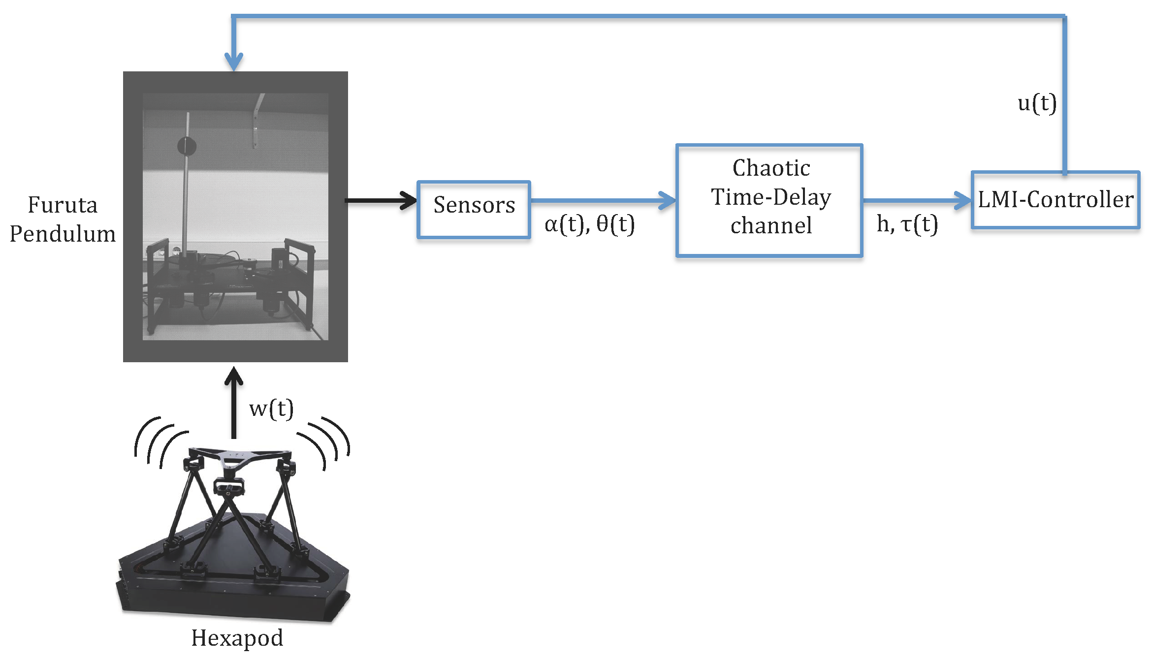
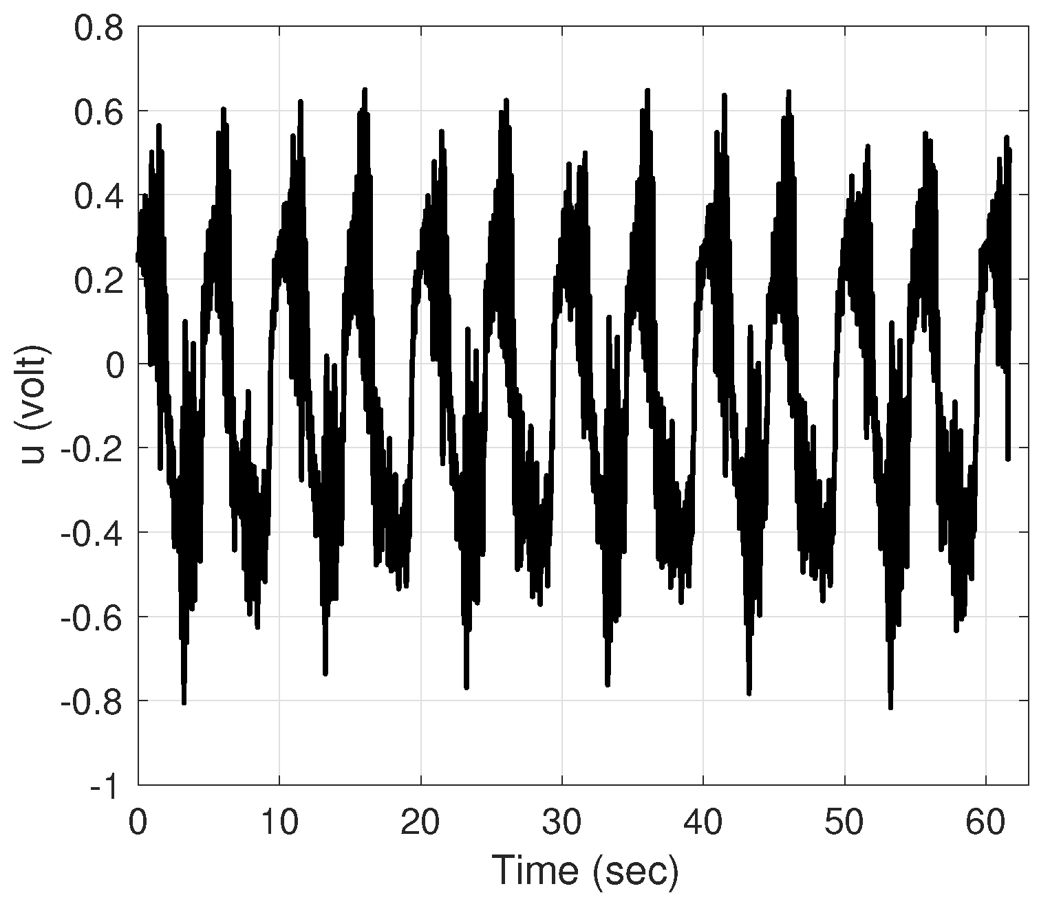
5. Experimental Results

This section presents the time delay Furuta pendulum experimental platform results, subject to exogenous disturbances. Figure 4 presents the random time delay introduced on the experimental system. The time delay is stated from logistic-map variable $x_n$, as defined in Algorithm 1. The delay takes values $\{0.02,0.4\}$ randomly, inducing some kind of chaotic behavior. Notice that the experimental sample-time is set at $0.885$ ms, so the time delay induced on the measurements is greater than the acquisition sample-time.

Additionally, at the link https://youtu.be/C8f1orF5uDo, the reader can find a demonstrative video of our experiment. The experiment begins without ground disturbance. Then, the external perturbation starts at 8s, when hexapod begins to move. Figure 5, Figure 6, Figure 7, Figure 8 and Figure 9 represent the state variables and control input seen in the video. The effect of the ground perturbation and how the control input tries to maintain the inverted pendulum in its upright position can be appreciated, despite time delay inputs and external disturbances. Therefore, Figure 5 shows a zoom to appreciate the reaction of the pendulum position when measurements are time delayed. Moreover, Figure 6 shows the disturbance produced by the hexapod, at the base of the system. The load position corresponding to $\theta \left(t\right)$ and pendulum position $\alpha \left(t\right)$ are pictured in Figure 7, and Figure 8 presents the control effort. Figure 9 shows that the random behaviour presented on the measurements does not appear on the Furuta system.

6. Conclusions

This paper presents a robust control design to a nonlinear system, against the presence of random time delay on the measurements, and exogenous disturbances. In our control approach, we develop a general design in terms of LMI, where the designer has to a priori define an upper bound of the allowed time delay. Hence, this value can be adjusted by an optimisation technique. Furthermore, a new experimental platform is realised, involving Furuta pendulum located over a Steward platform. Finally, according to experimental results, our control approach is able to attenuate random dynamics. Additionally, the video of the experiment can be found at https://youtu.be/C8f1orF5uDo.

Future work. In this paper, we consider only external perturbations that do not change the structure of the system. It can be an interesting future work to implement some fault structure detection directly on the pendulum and study the influence of the ground disturbance on it. Moreover, resilient control could be designed to recover its function after being damaged [54].

References

1. Zhang, R.; Hredzk, B. Distributed Finite-Time Multi-agent Control for DC Micro-grids With Time Delays. IEEE Trans. Smart Grid 2019, 10, 2692–2701. [Google Scholar] [CrossRef]
2. Liu, L.; Yin, S.; Zhang, L.; Yin, X.; Yan, H. Improved Results on Asymptotic Stabilization for Stochastic Nonlinear Time-Delay Systems With Application to a Chemical Reactor System. IEEE Trans. Syst. Man Cybern. Syst. 2017, 47, 195–204. [Google Scholar] [CrossRef]
3. Zappatore, A.; Augieri, A.; Bonifetto, R.; Celentano, G.; Savoldi, L.; Vannozzi, A.; Zanino, R. Modeling Quench Propagation in the ENEA HTS Cable-In-Conduit Conductor. IEEE Trans. Appl. Supercond. 2020, 30, 1–7. [Google Scholar] [CrossRef]
4. Buzhin, I.G.; Mironov, Y.B. Evaluation of Telecommunication Equipment Delays in Software-Defined Networks. In Proceedings of the 2019 Systems of Signals Generating and Processing in the Field of on Board Communications, Moscow, Russia, 20–21 March 2019. [Google Scholar] [CrossRef]
5. Shirai, J.; Yamaguchi, T.; Takaba, K. Remote visual servo tracking control of drone taking account of time delays. In Proceedings of the 56th Annual Conference of the Society of Instrument and Control Engineers of Japan (SICE), Kanazawa, Japan, 19–22 September 2017. [Google Scholar]
6. Lim, B.; Lee, J.; Jang, J.; Kim, K.; Park, Y.J.; Seo, K.; Shim, Y. Delayed Output Feedback Control for Gait Assistance With a Robotic Hip Exoskeleton. IEEE Trans. Robot. 2019, 35, 1055–1062. [Google Scholar] [CrossRef]
7. Ali, H.; Dasgupta, D. Effects of time delays in the electric power grid. In Proceedings of the 6th International Conference on Critical Infrastructure Protection (ICCIP), Washington, DC, USA, 19–21 March 2012; pp. 139–154. [Google Scholar] [CrossRef]
8. Zhang, X.M.; Han, Q.L.; Seuret, A.; Gouaisbaut, F.; He, Y. Overview of recent advances in stability of linaer systems with time-varying delay. IET Control. Theory Appl. 2019, 13, 1–16. [Google Scholar] [CrossRef]
9. Mobayen, S. Optimal LMI-based state feedback stabilizer for uncertain nonlinear systems with time varying uncertainties and disturbances. Complexity 2015, 21, 356–362. [Google Scholar] [CrossRef]
10. Sun, Z.Y.; Song, Z.B.; Li, T.; Yang, S.H. Output feedback stabilization for high-order uncertain feedforward time-delay nonlinear systems. J. Frankl. Inst.-Eng. Appl. Math. 2015, 352, 5308–5326. [Google Scholar] [CrossRef]
11. Mahmoud, M.S. Recent Progress in Stability and Stabilization of Systems with Time-Delays. Math. Probl. Eng. 2017, 2017, 7354654. [Google Scholar] [CrossRef] [Green Version]
12. Li, X.; Cao, J.; Ho, D.W.C. Impulsive Control of Nonlinear Systems With Time-Varying Delay and Applications. IEEE Trans. Cyber. 2020, 50, 2661–2673. [Google Scholar] [CrossRef]
13. Briat, C. Linear parameter-varying and time-delay systems. Anal. Obs. Filter. Control. 2014, 3, 5–7. [Google Scholar]
14. Li, S.; Ding, L.; Gao, H.; Liu, Y.; Huang, L.; Deng, Z. ADP-Based Online Tracking Control of Partially Uncertain Time-Delayed Nonlinear System and Application to Wheeled Mobile Robots. IEEE Trans. Cybern. 2020, 50, 3182–3194. [Google Scholar] [CrossRef] [PubMed]
15. Sayyad-Delshad, S.; Gustafsson, T. H observer design for uncertain nonlinear discrete-time systems with time-delay: LMI optimization approach. Int. J. Robust Nonlinear Control 2015, 25, 1514–1527. [Google Scholar] [CrossRef]
16. Krishnamurthy, P.; Khorrami, F. Prescribed-Time Output-Feedback Stabilization of Uncertain Nonlinear Systems with Unknown Time Delays. In Proceedings of the 2020 American Control Conference (ACC), Denver, CO, USA, 1–3 July 2020; pp. 2705–2710. [Google Scholar]
17. Tong, S.C.; Sheng, N. Adaptive fuzzy observer back-stepping control for a class of uncertain nonlinear systems with unknown time-delay. Int. J. Autom. Comput. 2010, 7, 236–246. [Google Scholar] [CrossRef]
18. Lien, C.H.; Yu, K.W.; Huang, C.T.; Chou, P.Y.; Chung, L.Y.; Chen, J.D. Robust H control for uncertain T-S fuzzy time-delay systems with sampled-data input and nonlinear perturbations. Nonlinear Anal. Hybrid Syst. 2010, 4, 550–556. [Google Scholar] [CrossRef]
19. Goodall, D.P.; Postoyan, R. Output feedback stabilization for uncertain nonlinear time-delay systems subject to input constraints. Int. J. Control 2010, 83, 676–693. [Google Scholar] [CrossRef]
20. Lakshmanan, M.; Bharathidasan; Senthilkumar, D.V. Dynamics of Nonlinear Time-Delay Systems; Springer Series in Synergetics; Springer: Berlin, Germany, 2011. [Google Scholar]
21. Banerjee, T.; Biswas, D. Time-Delayed Chaotic Dynamical Systems; Springer: Berlin, Germany, 2018. [Google Scholar]
22. Wang, H.; Wu, J.; Sheng, X.; Wang, X.; Zan, P. A new stability result for nonlinear cascade time-delay system and its application in chaos control. Nonlinear Dyn. 2015, 80, 221–226. [Google Scholar] [CrossRef]
23. Zhao, Z.; Lv, F.; Zhang, J.; Du, Y. H synchronization for uncertain time-delay chaotic systems with one-sided Lipschitz nonlinearity. IEEE Access 2018, 6, 19798–19806. [Google Scholar] [CrossRef]
24. Park, J.H.; Kwon, O.M. A novel criterion for delayed feedback control of time-delay chaotic systems. Chaos Solitons Fractals 2005, 23, 495–501. [Google Scholar] [CrossRef]
25. Sudha, K.R.; Santhi, R.V. Robust decentralized load frequency control of interconnected power system with generation rate constraint using type-2 fuzzy approach. Int. J. Elect. Pow. Energy Syst. 2011, 33, 699–707. [Google Scholar] [CrossRef]
26. Yu, S.; Yu, X.; Shirinzadeh, B.; Man, Z. Continuous finite-time control for robotic manipulators with terminal sliding mode. Automatica 2005, 41, 1957–1964. [Google Scholar] [CrossRef]
27. Hu, Q.; Shi, P.; Gao, H. Adaptive variable structure and commanding shaped vibration control of flexible spacecraft. J. Guid. Control Dyn. 2007, 30, 804–815. [Google Scholar] [CrossRef]
28. Huang, Y.; Wang, J.; Wang, F.; He, B. Event-triggered adaptive finite-time tracking control for full state constraints nonlinear systems with parameter uncertainties and given transient performance. In ISA Transactions; Elsevier: Amsterdam, The Netherlands, 2020. [Google Scholar]
29. Yi, X.; Guo, R.; Qi, Y. Stabilization of Chaotic Systems With Both Uncertainty and Disturbance by the UDE-Based Control Method. IEEE Access 2020, 8, 62471–62477. [Google Scholar] [CrossRef]
30. Gritli, H. LMI-Based Robust Stabilization of a Class of Input-Constrained Uncertain Nonlinear Systems with Application to a Helicopter Model. Complexity 2020, 2020, 7025761. [Google Scholar] [CrossRef] [Green Version]
31. Xin, Z.; Xiao, C.; Hou, T.; Shen, X. Robust H-Control for Uncertain Stochastic Systems with Impulsive Effects. Mathematics 2019, 7, 1169. [Google Scholar] [CrossRef] [Green Version]
32. Zhou, K.; Khargonekar, P.P. Robust stabilization of linear systems with norm-bounded time-varying uncertainty. Syst. Control. Lett. 1988, 10, 17–20. [Google Scholar] [CrossRef]
33. Xu, S.; Van Dooren, P.; Stefan, R.; Lam, J. Robust stability and stabilization for singular systems with state delay and parameter uncertainty. IEEE Trans. Autom. Control 2020, 47, 1122–1128. [Google Scholar]
34. Golestani, M.; Mohammadzaman, I.; Yazdanpanah, M.J.; Vali, A.R. Application of finite-time integral sliding mode to guidance law design. J. Dyn. Syst. Measur. Control 2015, 137, 114501. [Google Scholar] [CrossRef]
35. Golestani, M.; Mohammadzaman, I.; Yazdanpanah, M.J. Robust finite-time stabilization of uncertain nonlinear systems based on partial stability. Nonlinear Dyn. 2016, 85, 87–96. [Google Scholar] [CrossRef]
36. Barbosa, K.A.; Souza, C.E.; Trofino, A. Robust H2 filtering for uncertain linear systems: LMI based methods with parametric Lyapunov functions. Syst. Control Lett. 2007, 54, 251–262. [Google Scholar] [CrossRef]
37. Ngo, P.D.; Shin, Y.C. Modeling of unstructured uncertainties and robust controlling of nonlinear dynamic systems based on type-2 fuzzy basis function networks. Eng. Appl. Artif. Intell. 2016, 53, 74–85. [Google Scholar] [CrossRef]
38. Gahinet, P.; Apkarian, P. A linear matrix inequality approach to H control. Int. J. Nonlinear Control 1994, 4, 421–448. [Google Scholar] [CrossRef]
39. Boyd, S.; El Ghaoui, L.; Feron, E.; Balakrishnan, V. Linear Matrix Inequalities in System and Control Theory; SIAM: Philadelphia, PA, USA, 1994. [Google Scholar]
40. Hilhorst, G.; Pipeleers, G.; Michiels, W.; Swevers, J. Sufficient LMI conditions for reduced-order multi-objective H2/H control of LTI systems. Eur. J. Control 2015, 23, 17–25. [Google Scholar] [CrossRef] [Green Version]
41. Zong, G.; Xu, S.; Wu, Y. Robust H stabilization for uncertain switched impulsive control systems with state delay: An LMI approach. Nonlinear Anal.-Hybrid Syst. 2008, 2, 1287–1300. [Google Scholar] [CrossRef]
42. Leite, V.J.S.; Tarbouriech, S.; Peres, P.L.D. Robust H state feedback control of discrete-time systems with state delay: An LMI approach. IMA J. Math. Control Info. 2009, 26, 357–373. [Google Scholar] [CrossRef]
43. Sootla, A.; Zheng, Y.; Papachristodoulou, A. On the Existence of Block-Diagonal Solutions to Lyapunov and H Riccati Inequalities. IEEE Trans. Aut. Contr. 2020, 65, 3170–3175. [Google Scholar] [CrossRef] [Green Version]
44. Mei, W.; Zhao, C.; Ogura, M.; Sugimoto, K. Mixed H2/H control of delayed Markov jump linear systems. IET Control Theory Appl. 2020, 14, 2076–2083. [Google Scholar] [CrossRef]
45. Haddad, W.M.; Hui, Q.; Chellaboina, V. H2 optimal semistable control for linear dynamical systems: An LMI approach. J. Frankl. Inst.-Eng. Appl. Math. 2011, 348, 2898–2910. [Google Scholar] [CrossRef]
46. Caharija, W.; Pettersen, K.Y.; Bibuli, M.; Calado, P.; Zereik, E.; Braga, J.; Gravdhl, J.T.; Sorensen, A.J. Integral Line-of-Sight Guidance and Control of Underactuated Marine Vehicles, Theory, Simulations, and Experiments. IEEE Trans. Control Syst. Technol. 2016, 24, 1623–1642. [Google Scholar] [CrossRef] [Green Version]
47. Mobayen, S.; Pujol-Vazquez, G. A Robust LMI Approach on Nonlinear Feedback Stabilization of Continuous State-Delay Systems with Lipschitzian Nonlinearities: Experimental Validation. Iran J. Sci. Technol. Trans. Mech. Eng. 2019, 43, 549–558. [Google Scholar] [CrossRef]
48. Briat, C. Linear Parameter-Varying and Time-Delay Systems: Analysis, Observation, Filtering and Control. In (Section 5.6.7), Advances in Delay and Dynamics 3; Springer: Berlin, Germany, 2015. [Google Scholar]
49. Pujol, G. Reliable H control of a class of uncertain interconnected systems: An LMI approach. J. Syst. Sci. 2009, 40, 649–657. [Google Scholar] [CrossRef]
50. Model, E.C.P. Manual for A-51 inverted pendulum accessory (Model 220). In Educational Control Products; Ecpsystems: Pleasanton, CA, USA, 2003. [Google Scholar]
51. Pujol-Vazquez, G.; Acho, L.; Mobayen, S.; Napoles, A.; Perez, V. Rotary inverted pendulum with magnetically external perturbations as a source of the pendulum’s base navigation commands. J. Frankl. Inst.-Eng. Appl. Math. 2018, 355, 4077–4096. [Google Scholar] [CrossRef] [Green Version]
52. Boeing, G. Visual Analysis of Nonlinear Dynamical Systems: Chaos, Fractals, Self-Similarity and the Limits of Prediction. Systems 2016, 4, 37. [Google Scholar] [CrossRef] [Green Version]
53. Pareek, N.K.; Patidar, V.; Sud, K.K. Image encryption using chaotic logistic map. Image Vis. Comput. 2006, 24, 926–934. [Google Scholar] [CrossRef]
54. Wang, F.; Qian, Z.; Yan, Z.; Yuan, C.; Zhang, W. A Novel Resilient Robot: Kinematic Analysis and Experimentation. IEEE Access 2020, 8, 2885–2892. [Google Scholar] [CrossRef]
Figure 1. Experimental setup: Furuta pendulum located on a Steward platform.
Mathematics 08 02131 g001
Figure 2. Diagram of the perturbed random time delay system.
Mathematics 08 02131 g002
Figure 3. Diagram representation of Furuta pendulum with rotating base [50,51]: θ load disk angular position, α pendulum angle, u motor torque.
Mathematics 08 02131 g003
Figure 4. Random time delay model. The values of random variable x n determine the time delay τ . The maximum delay is set at h = 0.4 s.
Mathematics 08 02131 g004
Figure 5. Experimental results in the time interval [23, 35] s. It can be appreciated that when the time delay is about 0.4 s, the pendulum maintains its upright position.
Mathematics 08 02131 g005
Figure 6. Hexapod links programmed motion to produce the exogenous disturbances to the Furuta pendulum. This Figure only shows 6 s of the external perturbation, to clarify the hexapod movement (see the video: https://youtu.be/C8f1orF5uDo).
Mathematics 08 02131 g006
Figure 7. Load disk (left) and Pendulum (right) angular position response (closed-loop system).
Mathematics 08 02131 g007
Figure 8. Experimental control effort of the closed-loop system.
Mathematics 08 02131 g008
Figure 9. Pendulum position versus pendulum velocity.
Mathematics 08 02131 g009
Sample Availability: Samples of the compounds are available from the authors.
Publisher’s Note: MDPI stays neutral with regard to jurisdictional claims in published maps and institutional affiliations.