Fuzzy Multicriteria Decision Mapping to Evaluate Implant Design for Maxillofacial Reconstruction

Abstract

Technological advancements in healthcare influence medical practitioners as much as they impact the routine lives of the patients. The mandible reconstruction, which constitutes an important branch in facioplasty, has been a challenging task for medical professionals. As part of scientific innovation, tailor-made implants are valuable for sustaining and regenerating facial anatomy, as well as preserving the natural appearance. The challenge of choosing an acceptable implant design is a tedious process due to the growing number of designs with conspicuous effectiveness. The design should be agreeable, easy-to-design, sustainable, cost-effective, and undemanding for manufacturing. The optimal implant design can efficiently and effectively recover the structure and morphology of the flawed region. Evidently, among the many variants, the choice of appropriate design is one of the prevalent implant design problems and is still under consideration in most studies. This work is focused on the multiattribute decision-making (MCDM) approach to choosing the most effective implant design. The prevalence of subjectivity in decision-making and the presence of inconsistency from multiple sources emphasize the strategies that must take ambiguity and vagueness into account. An integrated MCDM methodology, assimilating two modern and popular techniques is adopted in this work. The preferred approach implements the Fuzzy Analytical Hierarchy Process based on the trapezoidal fuzzy number to extract the criteria weights in decision mapping and the Technique for Order of Preference by Similarity to Ideal Solution and VIKOR to assess design choices. A two-stage mechanism is the cornerstone of the established methodology. The first stage analyses the criteria from the point of view of the designer, the context of fabrication, and consumer experience. The second stage identifies the most viable and feasible design. The procedure applied in this analysis can be considered to choose the optimal implant design and to decide on areas of improvement that ensure greater patient experience.

1. Introduction

The enormous demand for medical implants has led to advances in the areas of biomaterials, engineering methods, and digital technologies [1]. Biomaterials are characteristic or engineered materials utilized to strengthen or substitute tissue, organ, or organic structure with a view to improving the well-being of patients [2]. Titanium and its combinations are among the few biomaterials that coordinate the human body’s prerequisite of supplanting bone tissue. Titanium alloys such as Ti6Al4V are considered to be the most favored metallic biomaterial for medical and healthcare applications [3]. They provide a remarkable blend of elevated resistance to weight ratio, acceptable density, and superior corrosion resistance, as well as they are biocompatible and have nonmagnetic properties. Moreover, an appreciable ascent in the manufacturing of tailor-fabricated titanium implants with finer structure and biomechanical assistance has been acknowledged in medical applications. To improve the quality of the patient’s life, facilitating and applying customized implants is essential. Additionally, the study of the implant regarding its design fitting accuracy, biomechanical properties, and manufacturing process is of paramount importance.

The maxillofacial reconstruction is regarded as a strenuous and important procedure by surgeons. This can be related to the patient’s strict anatomical specifications, the mandible curvature, and the effective recovery of chewing and oral functioning [4,5]. 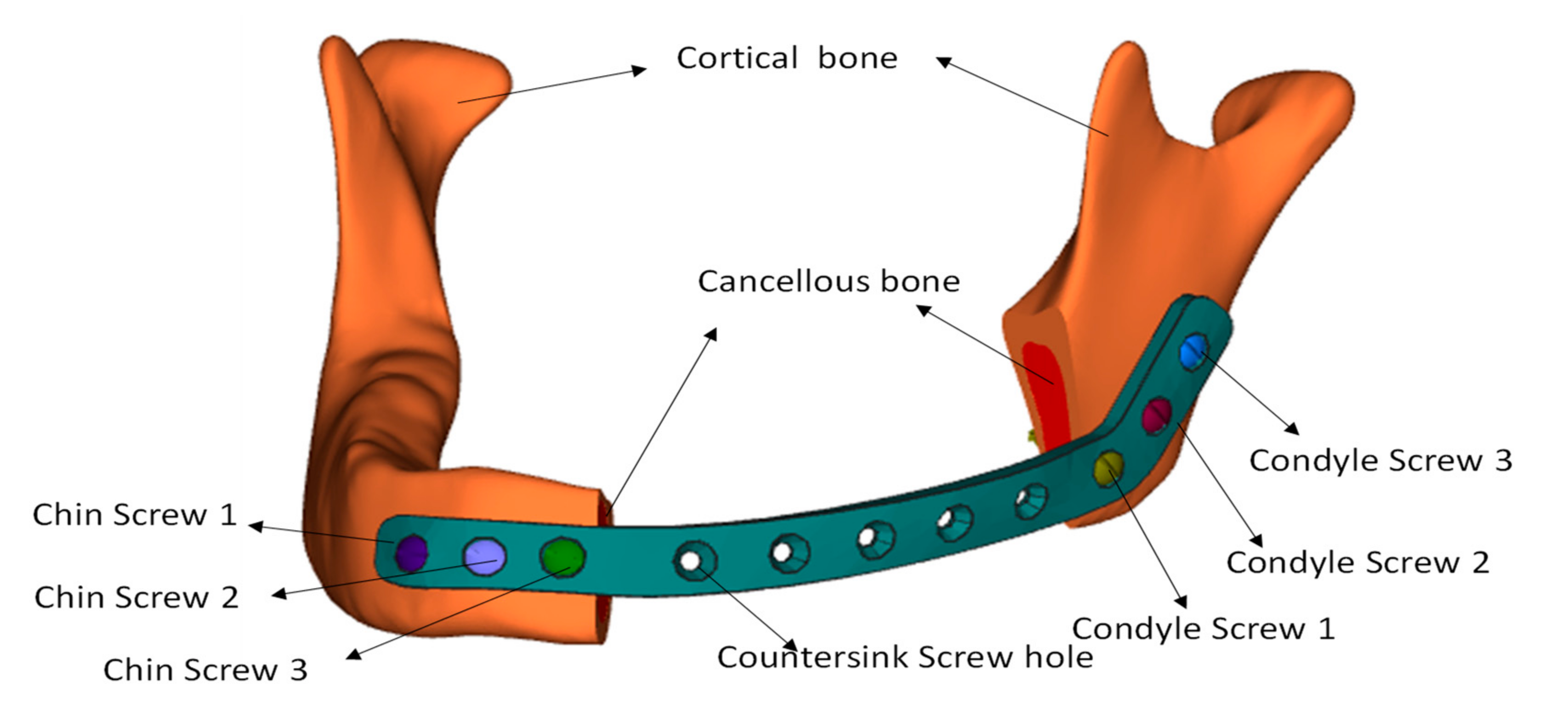The issue of mandibular reconstruction is even further exacerbated by a dramatic rise in mandibular abnormalities due to the complexity of the human body and evolving chewing behavior [6]. The abnormality of mandibular continuity generally involves bone loss in density caused due to trauma related oral lesions, tumors, etc. Prompt and effective recovery of mandibular defects is important in order to avoid deterioration of masticatory operation, voice loss, cosmetic imperfection, and to effectively accomplish the patient’s welfare. It is therefore important to use specially made implants that not only minimize disparity and incompatibility, but also improve the appearance and actualization. The specific implant configuration not only promotes the reliability of the fitting but also mitigates the processing time as compared to generic plates.

Apparently, implementing tailor-mandibular architecture requires developers to fully recognize the advantages and inconveniences of the various designs. Hence, due to the differential output and increased cost of various designs, it is necessary to choose the most viable design for a particular task. As reported by Baker et al. [7], it is only through a methodically formalized and well-defined philosophy that a worthwhile judgment (or selection) can be made. Certainly, multicriteria decision-making (MCDM) is one of those techniques and may be used to strengthen decision-making [8,9]. It is among the leading branches of operations research divisions comprising a set of deterministic possibilities estimated by a series of decision attributes [10]. During the last few decades, MCDM has noticed a plausible use [11]. It has evolved to meet various applications in the modern world such as supply chain management, finance, healthcare, factory location, environmental impact study, production, engineering, etc. [12]. This paper, therefore, applies the MCDM approach and analyzes its applicability in choosing the optimal design to achieve mandibular reconstruction. The adequate implant design is required so that the desired strength, stability, and surface area can be attained for better osseointegration. The accuracy is higher so that it suits precisely on the mandible and provides the optimal aesthetic. The reduced cost and manufacturing time make the design of the implant available to all patients. The implant design can be readily accessible when the design and manufacturing complexities are lesser. The lower weight increases both the patient’s comfort and exhaustion. Hence, it is necessary to select the optimal implant design that displays all the desired characteristics listed. The MCDM strategy is used to decide on an optimal option in the context of diverse and contradictory criteria. The goal of this analysis is to furnish medical and engineering professionals with basic information on the relevance of the implant design criteria to be implemented, that will ultimately lead to better decision-making and improved implant performance.

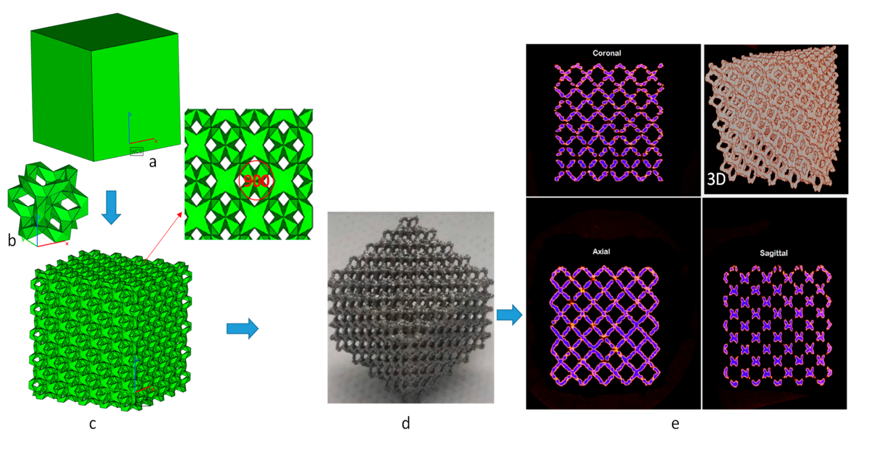
In the current implant industry, it is a standard practice that the design is chosen based on one or two criteria, overlooking the other variables. It is true that one design may be selected to satisfy specific requirements, but it may likely be possible that this design option does not perform well with other requirements. For example, among the four designs considered in this work, the analysis time, fabrication time, design, and manufacturing complexities for Design 1 are the lowest, but its stability is also the lowest. Similarly, if Design 3 is selected for some technological reasons, it provides very good stability, but the design complexity is very high. This study is carried out in such a way that most of the requirements are met by the one chosen implant design. For this purpose, all the criteria that are relevant to implant performance are identified. The possible criteria for implant design are established from the literature as well as by consultation with experts who provide opinions based on their expertise and experience. Based on the expert’s rating, the importance of each criterion in terms of weights is estimated. The collective decision-making (group of experts) approach is followed in this work to remove any bias in the decision model. The optimized implant design can then be selected from the available set of designs that can meet all the requirements or criteria. This research study takes into account four commonly used designs. Solid plate, sinewave, porous (top and bottom), and porous (inner) are the four designs. The list of criteria included Strength, Stability, Accuracy, Surface Area, Weight, Cost, Fabrication time, Design complexity, Manufacturing Complexity, Finite Element Modeling (FEM) analysis time, etc.

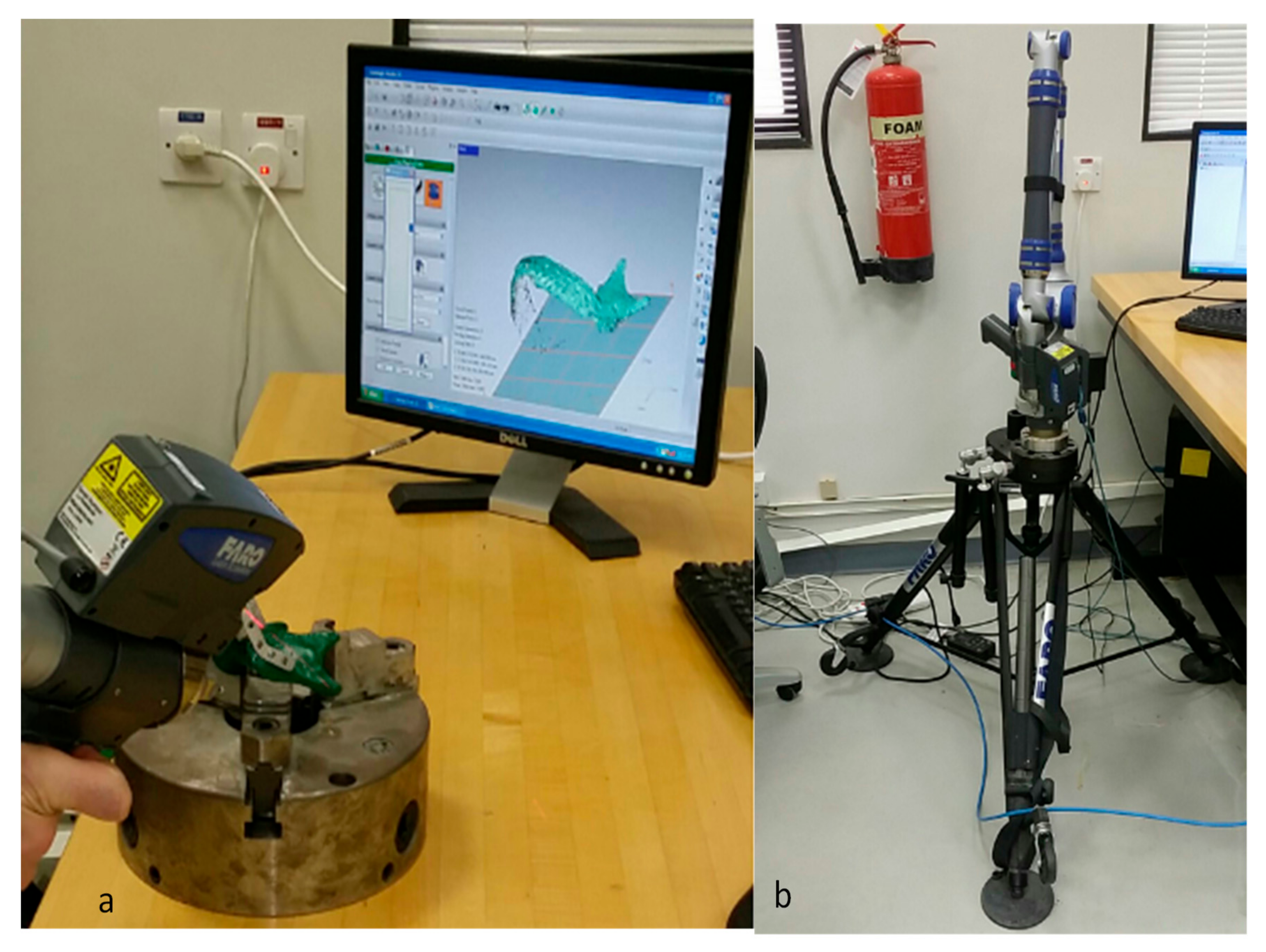
There are multiple criteria to evaluate the implant designs, so it can be described as an MCDM problem. It has many inputs, including qualitative and quantitative criteria, their values, opinions of experts, etc. The higher the precision of the different MCDM inputs, the better and more reliable the solution would be. There is, of course, a subjective element in the acquisition of opinions, and there is often a degree of ambiguity in data acquisition. For example, one of the criteria, stability, is evaluated by implementing a nondestructive scan-based micro-computed tomography (CT) technique. There are, however, many known and unknown variables that exist during micro-CT scans, and all of them cannot be considered during scanning. So, in the final result, there is always some degree of uncertainty. Hence, uncertainty and doubt in opinions and criteria assessment would have an impact on the quality of the results acquired. As a consequence, the method of Fuzzy Analytic Hierarchy Process (FAHP) has been adopted in this study to deal with incomplete, imprecise, and uncertain details ([13,14,15]). FAHP’s advantages are its ease of use and its willingness to recognize subjectivity, uncertainty, and inconsistency in individual decisions or weight estimation [16]. The two MCDM methods are used for grading various designs in order to ascertain the results derived from each other. The different fabricated designs are therefore evaluated using both FAHP-Techniques for Order of Preference by Similarity to Ideal Solution (TOPSIS) and FAHP-VlseKriterijumska Optimizacija I Kompromisno Resenje (VIKOR) to attain the optimum design.

The remainder of this paper is structured as below. The literature review is addressed in the accompanying Section 2. Section 3 and Section 4 describe the MCDM approaches and illustrate experimentation respectively. Section 5 define diverse criteria and analyze them by applying FAHP. The Section 6 describes the usage of TOPSIS and VIKOR in optimum design selection and Section 7 illustrates the conclusion part and future research work.

2. Literature Survey

Typically, regular commercial reconstruction plates (implants) are utilized in maxillofacial surgeries. Such plates are produced utilizing conventional techniques, like casting and metallurgical methods, that are often time-intensive procedures [17]. The standard plates are particularly straight and have to be bent to fit them around the contoured jaw bone. It not only increases the time of operation (or treatment) but also includes the painstaking process of constantly evolving and tweaking the plate depending on the patient’s physiology. As it is a random and rigorous practice, the likelihood of inconsistencies between the bone and plate interface accentuates, leading to implant malfunction and patient distress. It is therefore important to use personalized implants that not only mitigate the discrepancy and incompatibility, but also improve the look and the precision of the implants. The individualized implant design not only facilitates the accuracy of the fitting but also lessens the operative time as opposed to regular plates.

With innovations in technology, such as biomedical simulation software and three-dimensional (3D) printing or additive manufacturing, custom implants can now be more precisely designed and produced in a shorter time frame. The integration of data capture, imaging, design, and additive production has enabled the development of tailor-made implants depending on the patient’s current needs. The enactment of embedded technologies will undeniably save significant amounts of money for medical professionals and completely overhaul the living conditions of a significant number of people [18]. The satisfying impact of mandible reconstruction is heavily dependent on several implant dimensions including design manufacturing technology, biomechanical effects, precision, surface quality, and weight. There is no escaping the fact that 3D printing techniques offer exciting possibilities for bone reconstruction, regeneration, and surgery [19]. Electron beam melting (EBM) technology is a well-known process in the production of medical implants and devices and has received the European market approval (CE/Conformité Européene) and as well as food and drug administration approval (FDA) from United States [20]. EBM system, popularized in 1997 by ARCAM AB, produces parts in a layer by layer mode by fusing metal powder [21]. It can be satisfactorily used to build 3D titanium alloy scaffolds with sophisticated architecture for medical applications [22].

Maxillofacial bone is more of a twisted structure than a normal and uniform one. Correspondingly, few studies have tried to tailor the prosthesis configuration for mandibular reconstruction [23] and so little literature is available on maxillofacial scaffold analysis. Furthermore, there is no conclusive evidence and review concerning the choice of the correct mandibular prosthetic design. Numerous designs for mandibular reconstruction may be possible, such as a solid plate [24], Sinewave design plate [25], porous design [26,27], etc. The Solid plate is a common mandibular reconstruction plate matching the patient bone contours whereas the Sinewave plate is a new design plate that also matching the bone contours but in a sinewave design form. The porous design plates are scaffolds holding bone grafts. Preferably the scaffolds should be highly permeable, free of cracks, and biocompatible with tissue growth [28]. The titanium scaffolds can accomplish lifelong bone stabilization and support entire bone-in-growth in contrast to solid (bulk) bone growth, as illustrated in numerous research studies [29,30]. Furthermore, solid titanium implants can give rise to bone resorption owing to variations in mechanical properties, which causes the stress shielding implications on the adjacent bone and inevitably contribute to implant failure [31]. The exemplary porosity affects cell activity and the interconnected pores channels promote cell growth and rapid vascularization [32]. Promoting quick osseointegration is extremely important for successful implantation, otherwise longer cure time will result in implant malfunction [33]. Due to the uniqueness of different designs, it is important to choose the most appropriate design, and that is only possible through proper selection techniques, such as MCDM. MCDM provides an important decision-making mechanism that can be used in a variety of fields, in which finding the best option is incredibly complicated [34]. The literature seldom mentions research relating to the choice of custom mandible designs using MCDM. However, considerable work can be found in other domains where MCDM can be listed on the basis of either a single technique or its hybrid. Sadeghzadeh and Salehi, for example, applied the MCDM method in the automobile industry [35]. They researched multiple regulations for strategic fuel cell technologies and implemented TOPSIS to classify primary approaches for fuel cell technology advancement. Similarly, Ozcan et al. [36] suggested the principle of Analytic Hierarchy Process (AHP), TOPSIS, ELECTRE, and Grey to choose the appropriate warehouse location, despite high unpredictability and a range of products. Li et al. [37] conducted an assessment of coal mines to evaluate the non-risk working of mines. Weights for diverse criteria were estimated by exploiting the entropy technique, while TOPSIS was executed to assess coal mines depending on their safety situations. AHP is viewed as a widely used MCDM techniques [38]. The AHP, for instance, was implemented to achieve optimal maintenance solutions for the interactive learning and fabric industries by H. Fazlollahtabar and Yousefpoor [39] and Ilangkumaran and Kumanan [40], respectively. Bentes et al. [41] deployed a confluence of Balanced Scorecard (BSC) and AHP to improve the efficiency of the Brazilian telecom company. The BSC had been used to analyze varied performance measures and AHP was used to list the capabilities of the different operational divisions. With their inherent strengths and skills, there have been many approaches to MCDM. Consequently, they must be selected or implemented as required by the application. Pourjavad and Shirouyehzad [42] undertook detailed research on the three MCDM approaches TOPSIS, ELECTRE, and VIKOR for use in assembly channels. They studied the efficiency of simultaneous production facilities in the mining industry and examined the efficacy of MCDM methods.

Various fuzzy and conventional decision-making approaches are also helping health care and medical decisions. Sobolev et al. [43] proposed a computer-based simulation study in the analysis of surgical care delivery. Brailsford et al. [44] applied an integrated patient behavior simulation for the evaluation of breast cancer. Bahraminasab and Jahan [45] proposed a detailed VIKOR approach for the material choice in the femoral part of the entire knee replacements. Lee et al. [46] presented a fuzzy cognitive map of an MCDM approach in the acceptance of dental implant abutments. Cosma et al. [47] presented a computational intelligence approach, which included metaheuristic optimization algorithms for the prediction of prostate cancer and addressed its challenges. Baccour [48] proposed a novel integrated TOPSIS and VIKOR method for the categorization of heart diseases. Aenishaenslin et al. [49] presented a Preference Ranking Organization Method for Enrichment of Evaluations (PROMETHEE) MCDM approach to study Lyme diseases. Venhorst et al. [50] introduced a tool established on the nominal group technique and Delphi method for breast cancer interventions. Martinez et al. [51] employed the symmetrical triangular fuzzy approach to identify the titanium implant surface areas which influenced the implant performance. An expert-based questionnaire survey was performed to identify various implant properties on the biological, physicochemical, and mechanical performance. Nazari et al. [52] accomplished a clinical decision support advisor depending on a fuzzy interference system and FAHP to evaluate the patient’s condition and its diagnosis for heart diseases. Obanijesu and emuyibofarhe justice [53] designed a neuro-fuzzy system with eight inputs and one output for the detection of heart attacks. Banerjee et al. [54] recommended a unique combinatorial technique using fuzzy logic-based neural network models for the prediction of mechanical properties in orthopedic implants. It is interesting to know that most of the studies did not address group decision-making, the imprecision of expert views, and the uncertainty of the acquired criteria data. It is very complicated to weigh and also preserve the continuity of judgment using existing approaches, particularly with added criteria. These techniques needed a great deal of information and were unable to cope with incomplete information or knowledge. They required consistent preferences of the experts as well as precise details for high-quality results. These techniques did not deal with an incomplete amount of data and presumed that all measurements of output and input were defined.

It is clear that earlier publications seldom discussed research on the selection of acceptable implant design in mandibular reconstruction. Most researchers have suggested their specific implant designs (based on one or two aspects) for mandibular reconstruction. They did not, however, compare different designs using a robust decision-making approach like MCDM. Moreover, the earlier researches concentrated on one or two aspects of the design. Some designs, for example, were good in terms of stability; some were good in terms of design complexity, etc. The numerous criteria that may be very critical in the overall performance of the implant were overlooked in these studies. In order to create a better solution, a decision problem that includes a large number of criteria is especially useful. This research is therefore inspired by the need to resolve the constraint of fewer criteria when evaluating various designs. It is also evident from the literature that analysis on the application of MCDM in the selection of an effective design for mandibular reconstruction is rarely discussed. Thus, the need to demonstrate the successful application of MCDM in the implant industry also motivates this study.

Developing a cost-effective and differentiating custom mandibular design can be defined as a problem of optimization. It is because the selection of an optimal design can be affected by many factors. The presence of a wide variety of alternative design concepts therefore renders the selection process a complicated and nuanced activity [55]. A systematic approach is therefore required to assess a vast array of designs and recognize the most appropriate one. The combined use of multiple strategies is beneficial to prevent drawbacks and to take advantage of individual methods. The AHP is augmented with soft computing techniques such as fuzzy sets (FAHP) [56,57] and combined with TOPSIS/VIKOR approaches in this work to overcome the limitations of earlier initiatives. This approach is very beneficial since it can solve the problems of decision-making in an arbitrary and unpredictable setting and needs a minimal level of knowledge on criteria. The following sections demonstrate the application of MCDM methods when selecting an optimal design for mandibular reconstruction.

3. MCDM Approaches

This section introduces three strategies (FAHP, TOPSIS, and VIKOR) used in this work. The various mandible designs were developed at the outset. The performance of these designs was measured using various testing and analytical techniques. Appropriately, the TOPSIS [58] and VIKOR [59] based MCDM had been adopted to rank various designs.

3.1. Fuzzy Analytic Hierarchy Process

The indefiniteness and imprecision of expert viewpoints as well as experimental data were handled using Zadeh’s suggested principle of fuzzy sets [60]. The FAHP, which focuses on the concepts of Fuzzy set theory and hierarchical structural analysis, can systematically guide design selection. Nonetheless, the FAHP is an extension of a traditional AHP procedure by fuzzy numbers into a fuzzy setting [61]. Van Laarhoven and Pedrycz [62], Buckley [63], and Chang [64] suggested the initial transformation of the regular AHP into FAHP. They represented the relative priorities of the Saaty by deploying fuzzy numbers with triangular membership functions. Owing to its good performance and infrequent presence in earlier studies, the crisp values were modeled utilizing trapezoidal membership function in this investigation [65]. The various measures used in estimating fuzzy weights can be explored as below.

Step 1: Translation of crisp numbers into fuzzy values

In this step, the decision matrices were translated into trapezoidal fuzzy numbers (TrFNs). The membership function of F-designated TrFN characterized by (l, m, n, u) can be expressed as below [66,67].

$$\mathrm{Membership}\mathrm{function},{{\mu }_F}_{}(x)=\left\{\begin{array}{c}\begin{array}{cc}0& x\le l\end{array}\\ \begin{array}{cc}\frac{x-l}{m-l}& l\le x\le m\end{array}\\ \begin{array}{cc}1& m\le x\le n\end{array}\\ \begin{array}{cc}\frac{u-x}{u-n}& n\le x\le u\end{array}\\ \begin{array}{cc}0& x\ge u\end{array}\end{array}\right.$$

The crisp numbers predicated on the Saaty scale were formerly converted into triangular fuzzy numbers (TFNs) and afterward into TrFNs. The TFNs were transformed into TrFNs by constantly maintaining the upper and lower limits of the fuzzy numbers and expanding the middle number to a specific degree [68]. For instance, the crisp value of x can be transformed to a TFN (a, b, c) as a = x − 1; b = x and c = x + 1. The TFNs can subsequently be transformed into TrFNs (l, m, n, u) as l = a; u = c; m = l + 0.5 and n = u − 0.5.

Step 2: Computation of weights

The weights of the criteria were estimated by deploying the Chang extent analysis [64]. The extent analysis can be defined as follows for estimating prior weights [69,70]. Let X = {x₁, x_2, x_3, ……, x_n} denote the collection of entities and G = {g₁, g_2, g₃, ……, g_n} represent goals set. As stated by extent analysis methodology, every entity has to undergo extent analysis for each goal of the problem. Therefore, m extent analysis values for each entity can be acquired as below.

M¹_gi, M²_gi, M³_gi, M⁴_gi, ……, M^m_gi, i = 1, 2, 3, 4, …., n

where M^j_gi (j = 1, 2, 3, 4, … m) symbolizes TrFNs. The Chang’s extent analysis can be carried out in accordance with the following.

Concerning ith entity, the synthetic fuzzy values can be calculated by using Equation (1).

$$S_i={{\displaystyle \sum }}_{j=1}^m\begin{array}{ccc}{M}_{gi}^j& \otimes & {\left[{{\displaystyle \sum }}_{i=1}^n{{\displaystyle \sum }}_{j=1}^m{M}_{gi}^j\right]}^{-1}\end{array}$$

(1)

To estimate ${{\displaystyle \sum }}_{j=1}^m{M}_{gi}^j$, the fuzzy addition operation for a specific matrix can be accomplished utilizing the formulation in Equation (2).

$${{\displaystyle \sum }}_{j=1}^m{M}_{gi}^j=\left({{\displaystyle \sum }}_{j=1}^m{l}_j,{{\displaystyle \sum }}_{j=1}^m{m}_j,{{\displaystyle \sum }}_{j=1}^m{n}_j, {{\displaystyle \sum }}_{j=1}^m{u}_j\right)$$

(2)

The value of ${\left[{{\displaystyle \sum }}_{i=1}^n{{\displaystyle \sum }}_{j=1}^m{M}_{gi}^j\right]}^{-1}$ can be obtained through fuzzy addition operation of M^j_gi (j = 1, 2, 3, 4, …, m) values in the following manner using Equation (3).

$${{\displaystyle \sum }}_{i=1}^n{{\displaystyle \sum }}_{j=1}^m{M}_{gi}^j=\left({{\displaystyle \sum }}_{i=1}^n{l}_i,{{\displaystyle \sum }}_{i=1}^n{m}_i,{{\displaystyle \sum }}_{i=1}^n{n}_i, {{\displaystyle \sum }}_{i=1}^n{u}_i\right)$$

(3)

In addition, the inverse of the vector can be provided as in Equation (4).

$${\left[{{\displaystyle \sum }}_{i=1}^n{{\displaystyle \sum }}_{j=1}^m{M}_{gi}^j\right]}^{-1}=\left(\begin{array}{cccc}\frac{1}{{{\displaystyle \sum }}_{i=1}^n{u}_i},& \frac{1}{{{\displaystyle \sum }}_{i=1}^n{n}_i},& \frac{1}{{{\displaystyle \sum }}_{i=1}^n{m}_i},& \frac{1}{{{\displaystyle \sum }}_{i=1}^n{l}_i}\end{array}\right)$$

(4)

Assume M₁ = (l₁, m₁, n₁, u₁) and M₂ = (l₂, m₂, n₂, u₂) constitutes two TrFNs. The degree of possibility of M₂ = (l₂, m₂, n₂, u₂) ≥ M₁ = (l₁, m₁, n₁, u₁) are subject to following condition in Equation (5).

$$V(M_2\ge M_1)=\underset{y\ge x}{\sup }\left[\min \left({\mu }_{M_1}\left(x\right),{\mu }_{M_2}\left(y\right)\right)\right]$$

(5)

where, V (M₂ ≥ M₁) can be defined as follows in Equation (6)

$$V(M_2\ge M_1)=\mathrm{hgt}(M{1}_{}\cap M_2)={\mu }_{M_2}\left(d\right)=$$

$$\begin{array}{cc}1,& m_1\ge m_2\\ 0,& \left(m_2-n_1\right)>\left(u_1+l_2\right)\\ \frac{\left(\left(n_1-m_2\right)+\left(u_1+l_2\right)\right)}{\left(u_1+l_2\right)},& 0< \left(m_2-n_1\right)< \left(u_1+l_2\right)\\ \frac{\left(\left(m_2-n_1\right)+\left(u_1+l_2\right)\right)}{\left(u_1+l_2\right)},& \left(m_2-n_1\right)< \left(u_1+l_2\right), \mathrm{where} m_2<n_1 \mathrm{and} m_1<m_2 \end{array}$$

(6)

The degree of possibility of a fuzzy number higher than k fuzzy numbers can be described by means of

V (M₂ ≥ M₁, M_2, M₃, M₄, ……, M_k) = V [(M ≥ M₁) and V [(M ≥ M₂) and V [(M ≥ M₃) and V [(M ≥ M₄) and …… and V [(M ≥ M_k)] = min V (M ≥ M_i), i = 1, 2, 3, …, k.

Consider that d (A_i) = min V (S_i ≥ S_k) for k = 1, 2, 3, 4, …, n; k ≠ i. The weight vector can be demonstrated as follows in Equation (7).

$$w^{\prime }={\left(d^{\prime }\left(A_1\right), d^{\prime }\left(A_2\right),d^{\prime }\left(A_3\right),d^{\prime }\left(A_4\right),\dots ,d^{,}\left(A_n\right) \right)}^T$$

(7)

where A_i (i = 1, 2, 3, 4, …, n) are n elements. The normalization must be completed in order to attain the weight vectors for every element. The weight vectors are normalized to accomplish the normalized vectors.

$w$ = ${\left(d\left(A_1\right),d\left(A_2\right),d\left(A_3\right),d\left(A_4\right),\dots ,d\left(A_n\right)\right)}^T$, where w is a vector of non-fuzzy or crisp numbers.

3.2. Technique for Order Preference by Similarity to Ideal Solution

As mentioned in previous literature studies [71,72], a near-optimal solution is chosen by the TOPSIS. This leverages the notion of enlarging the distance from the ideal negative outcome and lowering the distance from the ideal positive outcome.

Let x_ij denote the value of variant i which corresponds to criterion j. A decision matrix that includes measures of different variants corresponding to their criteria can be described using Equation (8).

$$X={\left(x_{ij}\right)}_{s\mathrm{x}t}=\left[\begin{array}{ccc}{x}_{11}& \cdots & x_{1t}\\ ⋮& \ddots & ⋮\\ x_{s1}& \cdots & x_{st}\end{array}\right]$$

(8)

Let J denote the array of benefit criteria (i.e., higher is best), and let J′ be the cluster of negative attributes (less is good). TOPSIS is implemented as set out below.

• Development of a normalized matrix of decisions using Equation (9). This converts different dimensions of the attributes into non-dimensional attributes to allow their correlation.

$$r_{\mathrm{ij}}=x_{\mathrm{ij}}/\sqrt{\sum x_{ij}^2 }\mathrm{for}i=1,\dots ,s;j=1,\dots ,t$$

(9)

• Formation of the weighted, normalized matrix of decisions. Multiply every column of the standardized decision matrix by its weight. The element in the new matrix would attain the values according to Equation (10).

R_ij = w_j r_ij

(10)

• Estimation of both ideal and nonideal solution using Equation (11)

Positive Ideal Solution (PIS), A⁺ = {R₁⁺, R₂⁺, ……, R_s⁺};
R_j⁺ = {max_i (R_ij) if j ∈ J; min_i (R_ij) if j ∈ J’}
Negative Ideal Solution (NIS), A⁻ = {R₁⁻, R₂⁻, ……, R_s⁻};
R_j⁻ = {min_i (R_ij) if j ∈ J; max_i (R_ij) if j ∈ J’}

(11)

• Euclidean distances calculation from the PIS, A⁺ (benefits) and NIS, A⁻ (cost) of every option using Equation (12).

S_i ⁺ = [Σ (R_j⁺− R_ij)²] ^½   (i= 1, 2, …., s; j= 1, 2, …., t)
S_i⁻ = [Σ (R_j⁻− R_ij)²] ^½ (i= 1, 2, …., s; j= 1, 2, …., t)

(12)

• Estimation of the relative closeness with regard to PIS for every variant as given in Equation (13).

θ_i = S_i⁻/(S_i⁺ + S_i⁻), 0 < θ_i < 1

(13)

• Grade the variants by their relative proximity. The superior choice is the one with a greater value of θ_i, and thus should be preferred.

3.3. VIKOR Method

This subsection addresses the various steps required to implement the VIKOR-based MCDM technique [73]. Suppose that there are s variants S_i (i = 1, 2, …, s) and t criteria A_j (j = 1, 2, …, t). The VIKOR approach’s central idea is to ascertain the positive and negative idealized positions in the solution domain.

• Establish the decision matrix X = (x_ij)_s×t where x_ij denote real numbers characterizing the values of the jth criteria for the variant i.
• Compute the normalized decision matrix, (r_ij)_s×t utilizing Equation (14).

$${\left(r_{ij}\right)}_{s\times t}=\frac{x_{ij}}{\sqrt{\sum {\left(x_{ij}\right)}^2}}$$

(14)

• Define the maximum and minimum values in the normalized decision matrix using Equation (15).

$$\begin{gathered} v_j^{+}=\underset{j}{\max }{r}_{ij}\mathrm{and}{v}_j^{-}=\underset{j}{\min }{r}_{ij}\mathrm{for}\mathrm{benefit}\mathrm{criterion} \\ {v}_j^{+}=\underset{j}{\min }{r}_{ij}\mathrm{and}{v}_j^{-}=\underset{j}{\max }{r}_{ij}\mathrm{for}\mathrm{non}-\mathrm{benefit}\mathrm{criterion} \end{gathered}$$

(15)

• Calculate the distance of variants to the ideal solution, which is the criterion of utility (S_i) and the estimate of regret (R_i) employing Equation (16).

$$S={{\displaystyle \sum }}_{j=1}^t{w}_j\frac{v_j^{+}-v_{ij}}{v_j^{+}-v_j^{-}}\mathrm{and}{R}_i=\underset{j}{\max }(w_j\frac{v_j^{+}-v_{ij}}{v_j^{+}-v_j^{-}})$$

(16)

• Calculate the values for Q_i (rank indexes) using Equation (17).

$$Q_i=\left(\phi \ast \frac{S_i-S^{+}}{S^{-}-S^{+}}+\left(1-\phi \right)\ast \frac{R_i-R^{+}}{R^{-}-R^{+}}\right)$$

(17)

where, S⁺ = $\underset{i}{\mathit{min}}{S}_i$ S⁻ = $\underset{i}{\mathit{max}}{S}_i$ R⁺ = $\underset{i}{\mathit{min}}{R}_i$ R⁻ = $\underset{i}{\mathit{max}}{R}_i$

$\varnothing$ ∈ [0, 1] symbolizes the weight for the strategy of “the majority criteria” (or “the maximum group utility”). The rate of quality is based on the S_i values and the worst score is dependent on R_i values.

• Grade the variants in increasing order depending on the Q_i values.

The solution (Q_minimum) recommended by the VIKOR procedure is further evaluated to meet the following requirements [73,74]:

C1. Acceptable advantage

Q₁ − Q₂ ≥ DQ, where i = 2 is the ranking’s second-best option using Q and DQ = 1/(s − 1).

C2. Acceptable stability

The variant i = 1 has to be ranked as best by R and/or S. It suggests a set of alternative options in case either of the criteria is not fulfilled.

• Variants i = 1 and i = 2 if only condition C₂ is not attained, or
• Variants i = 1, 2, …, s, if the condition C₁ is not met, where s is determined by the Q_S − Q₁ < DQ relationship, for maximum i.

3.4. Sensitivity Analysis

The sensitivity analysis is applied to ascertain the resilience and consistency of estimated ranking. It can be characterized as a procedure for analyzing the influence of input values on the eventual outcomes of the model [75]. It is definitely important to analyze the anomalies in the outcome variables of the given model due to fluctuations in the values of the input parameters [76,77]. This means that the model is robust and efficient if the model outcome is not very responsive to input changes. The most frequently employed sensitive analysis is carried out by altering the weights of the output indicators and evaluating the impact on the output [78]. Prior findings have also showcased that the selection of appropriate option relies considerably on the weight coefficients of the criterion [79]. Consequently, in this analysis, sensitivity analysis due to fluctuations in weight coefficients was conducted to validate the model and guarantee the robustness of results.

The arbitrary selection of a criterion was the initial stage in the sensitivity analysis. This was accompanied by a percentage shift in the chosen criterion weight (more or less). Then, the weights for the residual criteria were estimated by employing Equation (18) [80].

$$w_t^{*}=\frac{w_t\left(1-w_i^{*}\right)}{\left(1-w_i \right)}$$

(18)

where

• w_i: Actual weights for criteria i
• w_i^*: Weight attained after modifying the actual weight by 10% for criteria i
• w_t: Actual weight for criteria t
• w_t: Estimated weight for criteria t

Kendall’s coefficient (W) of concordance was implemented to gauge the effectiveness of the established method and to visualize the correlations of ranks produced by differing weights [81,82]. The measure of W expresses the commonalities in the ranking and it varies from 0 to 1. The value of 1, for instance, indicates an ideal match between the different ranking orders. This means that the nearer the value of W to 1, the higher the reproducibility would be. By leveraging Equations (19)–(21), the value of W can be derived as below.

$$W=\frac{12R}{m^2 \left(k^3-k\right)}$$

(19)

$${R_i}_{}={{\displaystyle \sum }}_{j=1}^m{r}_{ij}$$

(20)

$$R={{\displaystyle \sum }}_{i=1}^k{\left(R_i-\overline{R}\right)}^2$$

(21)

where r_ij = ranking scenario i for variant j, m = count of scenarios and k = count of variants.

Three schemes (20%, 30%, and 40%) were developed based on weight percentage. There were 10 scenarios relying on variably chosen criteria for the percentage change in each scheme. In

Table 1. Scenarios used in sensitivity analysis.

Scenario	Description
1	Percentage weight increment for implant weight
2	Percentage weight reduction for implant stability
3	Percentage weight reduction for fabrication time
4	Percentage weight increment for accuracy
5	Percentage weight increment for design complexity
6	Percentage weight reduction for cost
7	Percentage weight reduction for Finite Element Modeling (FEM) analysis time
8	Percentage weight reduction for manufacturing complexity
9	Percentage weight increment for surface area
10	Percentage weight increment for strength

, the various schemes and scenarios can be observed. Scheme 2 and scenario 3, for example, reflect a 30% reduction in weight for fabrication time (weights of the residual criteria were estimated using Equation (18)).

4. Experimentation

This segment addresses the methodology employed to obtain the values for various criteria. A total of four different mandibular reconstruction plates were designed and fabricated using a similar methodology. The process flow, as demonstrated in Figure 1, illustrates the approach used in this study. It was depended on the following phases: patient’s CT scan, data acquisition, data processing, customized implant design, virtual assembly, finite element analysis (FEA), Standard Tessellation Language (STL) corrections, implant fabrication, and implant post-processing.

4.1. Data Acquisition

The data were obtained from a patient with deformities in the left mandibular region. The CT scan was performed on the patient by a Planmeca Promax 3D (Helsinki, Finland) Cone Beam Computed Tomography (CBCT) machine [83]. The digitized medical images were collected as Digital Imaging and Communications in Medicine (DICOM) files composed of two-dimensional (2D) header and image data sets, all bundled in one file. The images stored in DICOM were then used to model custom mandibular implants. MIMICS 17.0^® (Materialise NV, Leuven, Belgium) was used to transform the DICOM into a 3D model [84] (see Figure 2a). For bone categorization, a modular Hounsfield unit (HU) ranging from 226 to 16950 was enforced. The region growing tool had been used to fragment the entire face mask into a set of specific entities (Figure 2b) until the desired region (mandible) was extracted (Figure 2c). The consequent operation Figure 2d) was to detach the teeth to obtain the bony mandibular region (Figure 2e). The tumor in the left mandibular region (Figure 2f) was then trimmed using the MIMICS^® cut and punch tool feature to obtain the resected mandible (Figure 2g). The cancellous and cortical bones (Figure 2h) were segregated from the resected mandible using MIMICS^® erode method. Finally, the resected mandible with cortical and cancellous bone (Figure 2i) were stored as an STL file.

4.2. Customized Implant Design and Modeling

The resected STL file (Figure 3a) was imported into a 3-Matic^® (Materialise, Leuven, Belgium) medical implant modeling program for tailor mandibular implant construction. The mirror reconstruction method, which is one of the widely used techniques for anatomy reconstruction, was used to replace the affected area with the healthy region [85]. In this step, the resected mandible was first trimmed using cut and punch operation (Figure 3b) and divided into two unconnected sections (Figure 3c). The deficient region on the left (green) had been removed (Figure 3d) and mirroring was implemented to fill the gap with the normal region (Figure 3e). Merge and wrap procedure was carried out to remove the gaps and voids between the left and right mandibular regions (Figure 3f).

The retrieved healthy mandible (Figure 3g) was then used by filtering (Figure 3h) and for the extraction of outer bone area for custom implant design (Figure 3i). Trimming and cutting operations were conducted to obtain the shape of the implant design that served as a custom implant prototype. All 4 implant design models provided a thickness of 2 mm. The first customized implant design was a common straight reconstruction plate matching the bone contours (Figure 3j) whereas the second plate was a new sinewave (zigzag) reconstruction plate (Figure 3k) also matching the bone contours. The third and fourth reconstruction plates were the bone graft carriers attached to the straight reconstruction plate in which the graft carrier was converted from a solid to porous. The third reconstruction plate was named as top and bottom porous plate because the solid top and bottom regions were converted from solid to porous (Figure 3l). In the fourth reconstruction plate, the inner bone graft carrier was converted from solid to porous and hence named as an inner porous plate (Figure 3m). In this design, the porous structure is attached on the inner side of the plate. The main difference between the two is the attachment of a porous structure. Several research papers have shown that 500–1000 micron titanium porous scaffolds promote implant-bone growth and rapid bone healing [86,87].

4.3. Virtual Assembly

As shown in Figure 4, the four custom-crafted mandibular plates were virtually aligned and mounted to the mandibular framework model for fitting evaluation. The first revision and formal meetings between the engineering and medical field were held to review and approve the implant designs. The designed implants proceeded to the next stage when approved by the physician. Any error between bone and implant design interface would result in redesigning implants.

Figure 5 demonstrates the holistic perspective of the mandibular frame model’s virtual assembly. It consisted of the cortical and cancellous bone with a mandibular implant fitted with six screws, three condyle side screws, and three chin area screws. Countersink holes were designed to ensure patient’s satisfaction and provide a better aesthetic effect. The four mandibular implant designs and the mandibular structure template were saved for FEA as a Standard for the Exchange of Product Data (STEP) file.

4.4. Finite Element Analysis

The FEA offers a powerful approach for the prediction of real-world scenarios under various loading and boundary conditions [88]. The FEM consisted of 4 developed titanium plates, as well as the mandibular frame model (cortical and cancellous bone) and bi-cortical medical titanium screws to test the biomechanical analysis of the engineered implants under clinching (chewing) conditions. In this study, the 3 mandible muscular forces (masseter, medial pterygoid, and temporalis) and the sustained clenching were simulated. The masticatory forces applied by each muscle along the direction under chewing simulation are depicted in Figure 6. The material properties of the titanium reconstruction plates, cortical bone, cancellous bone, and titanium screws for the FEA as shown in

Table 2. Material properties utilized in FEM [89,90].

Materials	Young’s Modulus (MPa)	Poisson’s Ratio	Yield Strength (MPa)
Cortical Bone	13,700	0.3	122
Cancellous Bone	1370	0.3	2
Prosthesis scaffold, (Ti6Al4V ELI)	120,000	0.3	930

were taken from previous literature studies [89,90].

In clenching simulation, the boundary conditions and the magnitude of the muscular forces were taken from the literature studies [91,92] and are presented in

Table 3. Measure and direction of masticatory muscles [91,92].

Masticatory Muscles	X (Newton)	Y (Newton)	Z (Newton)
Masseter	50	−50	200
Medial pterygoid	0	−50	100
Temporalis	0	100	200

.

The titanium reconstruction plates were assumed to fail if it surpasses the yield strength of the built titanium material (800 MPa). Figure 7 illustrates the results of von Mises stresses of the four designed reconstruction plates. All the 4 designed reconstruction plates had successfully withstood the muscular forces under chewing conditions. The maximum von Mises stress among the 4 reconstruction plates was noticed in the Inner porous plate (360.22 MPa) and least von Mises stress in the sinewave rehabilitation plate (168.79 MPa).

4.5. Fabrication

In this study, the custom implants were fabricated using titanium material. The ARCAM’s EBM machine as demonstrated in Figure 8b was utilized for the production of titanium implants. The EBM working theory and concepts are reported in L.E. Murr [93] and Hopkins and dickens [94]. EBM is a powder bed fusion process in which the parts were fabricated in the following phases: (1) metal powder preheating, (2) scanning and melting, and (3) built platform movement and powder raking. The three steps were repeated in a loop until the desired end object was produced. Upon completion of the built object, the fabricated parts were loaded onto the powder recovery system (PRS, Figure 8a) to get rid of the support structures and semi-sintered powder adhered to it. Figure 8c illustrates the EBM-fabricated titanium implants which can be sterilized before final surgery.

4.6. Evaluation and Validation

Eventually, the manufactured titanium scaffolds were examined to determine various attributes, namely stability, accuracy, weight, and cost.

4.6.1. Stability through Micro-CT Scan

A micro-CT scan-based nondestructive technique was used to investigate stochastic defects and structural integrity of the mesh form employed in the scaffold. In addition to evaluating the interior architecture of the built struts, the micro-CT scans were exploited to evaluate the structure in terms of fractures, internal stuck debris, etc. A 15 mm solid cube (Figure 9a) was modeled and converted to a porous cube (Figure 9c) using a dode-thick porous mesh (Figure 9c) and manufactured by utilizing EBM. The micro-CT scanner (Bruker Skycam 1173, Kontich, Belgium) was used to analyze the EBM manufactured cube structure (Figure 9d). The micro-CT scan results (Figure 9e) illustrated that the manufactured scaffold was free from any cracks and was interconnected with a series of network channels. Similar results of the porous mandibular plate with top and bottom scaffolds were expected with the dode-thick structure. Further investigation and consultation with the maxillofacial surgeons reported that the top and bottom porous plate had better stability when compared to the inner porous plate. Certainly, they recommended the top and bottom porous plate design in contrast to the inner porous plate due to their higher compactness, control, and grip on the human anatomy.

4.6.2. Accuracy with 3D Comparison

The 3D comparison procedure was used to analyze the fitting quality of various designs with regard to the mandible as shown in Figure 10. The Geomagics Control^® was utilized to estimate the fitting accuracy [95]. The 3D comparison technique can be postulated amongst the effective and accurate methods for visually representing the surface irregularities between the restored components and their CAD reference counterpart [96]. The metric “average deviation” was used in this study to evaluate the proper fitting of the implants on the mandible. The test model was captured in the form of a point cluster using the laser scanner fixed on the Faro Platinum arm (FARO, FL, USA) as depicted in Figure 11b.

The implants were placed on the mandible and digitized to capture the test model as observed in Figure 11a. The reference model developed through the mirroring method was anticipated to demonstrate the ideal anatomical shape. The 3D analysis interpreted the outcome by estimating the lowest distance between the reference and the test models.

4.6.3. Weights of the Scaffold Designs

The weight of the mandibular bone region to be substituted was determined utilizing the density formula. The volume for weight estimation was estimated from the software Magics^® (Materialise, Leuven, Belgium) and the density was presumed to be 1600 kg/m³ [97]. The weights of the 4 reconstruction plates manufactured by EBM were recorded using a digital weighing system and are presented in

Table 4. Weight of EBM reconstruction plates and substituted mandibular bone portions.

Parts	Replaced Bone	Design-1	Design-2	Design-3 (Top and Bottom)	Design-4 (Inner Porous)
Volume (mm3)	11,879.00	1601	1538	2016.00	1847.00
Weight (grams)	19.00	6.10	5.73	10.67	8.14

.

5. Criteria of Different Designs

The criteria can be classified either as benefits or as cost criteria. The benefit criteria can be defined as those requirements which demand higher values, i.e., they exhibit a positive impact on performance. For example, strength, stability, and surface area are criteria of benefit in this research. Likewise, cost criteria have a negative influence, which is that the performance deteriorates if its values rise. The FEM analysis time, average deviation (accuracy), weight, cost, fabrication time, design complexity, and manufacturing complexity can be classified as cost criteria. The cost of the implant (in dollars, including the cost of the materials, software setup, etc.) was estimated by the cost model. The stability, accuracy, and weight were determined through micro-CT scan, 3D comparison, and weight measurement as discussed in the previous section. The strength and analysis time were computed using FEA simulation, while the surface area was estimated through software calculation. The design complexity and manufacturing complexity depended on the literature surveys, user experience, number of parameters involved, etc. They define the ease of design of the implant. The different criteria and their respective values may be outlined in

Table 5. Different designs and their attribute values.

Variants	Criteria
	C1	C2	C3	C4	C5	C6	C7	C8	C9	C10
	Strength	Stability	FEM Analysis Time	Accuracy	Surface Area	Weight	Cost	Fabrication Time	Design Complexity	Manufacturing Complexity
Design1	267.21	Low	0.86	1.0046	2263	6.07	1.34	60	Low	Low
Design2	168.79	Average	0.93	1.2146	2192	6.1	1.342	70	Average	Low
Design3	214.77	Very High	2.58	0.9953	6653	8.14	1.7908	90	Very High	Average
Design4	360.22	High	2.68	1.30747	9108	10.67	2.3474	121	High	Average

.

The different levels of the intangible criteria, namely, stability, design complexity, and manufacturing complexity were assured depending on knowledge and experimentation. The intangible criteria are regarded as criteria that are not measurable on a well-defined scale. As shown in

Table 6. Scale for intangible criteria.

Cost Attributes	Scale	Benefit Attributes
Very high	1	Very low
High	3	Low
Average	5	Average
Low	7	High
Very low	9	Very High

, the levels were thus defined using the scale for intangibles.

Table 7. Different designs and their corresponding attribute values.

Variants	Criteria
	C1	C2	C3	C4	C5	C6	C7	C8	C9	C10
	Strength	Stability	FEM Analysis Time	Accuracy	Surface Area	Weight	Cost	Fabrication Time	Design Complexity	Manufacturing Complexity
Design1	267.21	3	0.86	1.0046	2263	6.07	1.34	60	7	7
Design2	168.79	5	0.93	1.2146	2192	6.1	1.342	70	5	7
Design3	214.77	9	2.58	0.9953	6653	8.14	1.7908	90	1	5
Design4	360.22	7	2.68	1.30747	9108	10.67	2.3474	121	3	5

outlines the various criteria that were established using experiments, software calculation, and expert opinions. The values of intangible requirements are also displayed in this table.

There were 4 experts whose experience and expertise were applied to decide and weigh different criteria necessary to choose an optimal design. A decision matrix depending on expert opinions was accomplished utilizing Saaty’s intensity scale as illustrated in

Table 8. Saaty’s intensity importance scale [98].

Importance Scale	Explanation
1	Equal Importance
3	Moderate Importance
5	Strong Importance
7	Very Strong Importance
9	Extreme Importance
	The following represent the intermediate values
2	More than Equal Importance but less than Moderate Importance
4	More than Moderate Importance but less than Strong Importance
6	More than Strong Importance but less than Very Strong Importance
8	More than Very Strong Importance but less than Extreme Importance
Reciprocal values	If an element has any of the above non-zero numbers assigned to it in comparison to its element j, then j has the reciprocal value in comparison to i.

. The group of diverse experts (4 experts) assessed the criteria in this work because a single expert provides limited expertise and experience. The weights from the individual experts were aggregated to get combined weight. The goal of this approach was to find an ideal expert with the highest degree of decision consistency, the most accurate assessment, and whose evaluation was aligned with those of the other experts in the group. This method of group criteria weights guaranteed that the relevance of the criteria and therefore the final chosen implant design met the specifications from the point of view of experts.

The decision matrices for 4 experts were obtained as the outcome of this phase. The data collected from various experts were validated to conform their consistency prior to further processing [99]. In order to analyze the reliability of decisions, Saaty [98] introduced a random consistency index (RI) depicted in

Table 9. Random consistency index.

n	1	2	3	4	5	6	7	8	9	10
RI	0	0	0.58	0.9	1.12	1.24	1.32	1.41	1.45	1.49

. The consistency ratio, CR that correlates the consistency index (CI) with the RI must be described as below.

$$\mathrm{CR}=\frac{CI}{RI},\mathrm{where}\mathrm{CI}=\frac{{\lambda }_{max}-n}{n-1}$$

The λ_max specifies the decision matrix’s maximum eigenvalue and n denotes the count of attributes. If CR is less than or equal to 10%, the discrepancy is permissible, otherwise expert must amend their decision matrix.

6. Selection of Design

The potential benefit of choosing the optimal design had to do specifically with patient satisfaction. The choice of the best design for the given application drives the patient’s level of satisfaction. Random design selection can lead to a higher cost-benefit ratio. A combination of various MCDM methods was applied to get the optimal design. The systematic procedure pursued to accomplish the desired implant design is outlined in Figure 12.

To calculate the weights of different criteria, a group of four experts graded different criteria on a scale of 1 to 10, with 1 being the lowest priority and 10 being the utmost priority.

Table 10. Rating of attributes by experts.

Criteria	Experts
	E1	E2	E3	E4
Strength, C1	7	9	6	6
Stability, C2	9	7	8	9
FEM analysis time, C3	4	8	5	3
Accuracy, C4	9	9	8	7
Surface Area, C5	3	6	3	4
Weight, C6	7	7	8	8
Cost, C7	7	5	9	9
Fabrication time, C8	4	7	3	4
Design Complexity, C9	4	7	3	5
Manufacturing Complexity, C10	3	7	2	3

presents the ranking results thus recorded.

The goal behind several experts was to combine more than one professional’s opinions to remove any prejudice. The decisions of the consultants were converted into decision matrices as shown in

Table 11. Comparison of different criteria for different experts.

E1	C1	C2	C3	C4	C5	C6	C7	C8	C9	C10
C1	1	0.3333	4	0.3333	5	1	1	4	4	5
C2	3	1	6	1	7	3	3	6	6	7
C3	0.25	0.1667	1	0.1667	2	0.25	0.25	1	1	2
C4	3	1	5.9988	1	7	3	3	6	6	7
C5	0.2	0.1429	0.5	0.1429	1	0.2	0.2	0.5	0.5	1
C6	1	0.3333	4	0.3333	5	1	1	4	4	5
C7	1	0.3333	4	0.3333	5	1	1	4	4	5
C8	0.25	0.1667	1	0.1667	2	0.25	0.25	1	1	2
C9	0.25	0.1667	1	0.1667	2	0.25	0.25	1	1	2
C10	0.2	0.1429	0.5	0.1429	1	0.2	0.2	0.5	0.5	1
E2	C1	C2	C3	C4	C5	C6	C7	C8	C9	C10
C1	1	3	2	1	4	3	5	3	3	3
C2	0.3333	1	0.5	0.3333	2	1	3	1	1	1
C3	0.5	2	1	0.5	3	2	4	2	2	2
C4	1	3.0003	2	1	4	3	5	3	3	3
C5	0.25	0.5	0.3333	0.25	1	0.5	2	0.5	0.5	0.5
C6	0.3333	1	0.5	0.3333	2	1	3	1	1	1
C7	0.2	0.3333	0.25	0.2	0.5	0.3333	1	0.3333	0.3333	0.3333
C8	0.3333	1	0.5	0.3333	2	1	3.0003	1	1	1
C9	0.3333	1	0.5	0.3333	2	1	3.0003	1	1	1
C10	0.3333	1	0.5	0.3333	2	1	3.0003	1	1	1
E3	C1	C2	C3	C4	C5	C6	C7	C8	C9	C10
C1	1	0.3333	2	0.3333	4	0.3333	0.25	4	4	5
C2	3.0003	1	4	1	6	1	0.5	6	6	7
C3	0.5000	0.25	1	0.25	3	0.25	0.2	3	3	4
C4	3.0003	1	4	1	6	1	0.5	6	6	7
C5	0.25	0.1667	0.3333	0.1667	1	0.1667	0.1429	1	1	2
C6	3.0003	1	4	1	5.9988	1	0.5	6	6	7
C7	4	2	5	2	6.9979	2	1	7	7	8
C8	0.25	0.1667	0.3333	0.1667	1	0.1667	0.1429	1	1	2
C9	0.25	0.1667	0.3333	0.1667	1	0.1667	0.1429	1	1	2
C10	0.2000	0.1429	0.25	0.1429	0.5	0.1429	0.125	0.5	0.5	1
E4	C1	C2	C3	C4	C5	C6	C7	C8	C9	C10
C1	1	0.25	4	0.5	3	0.3333	0.25	3	2	4
C2	4	1	7	3	6	2	1	6	5	7
C3	0.25	0.1429	1	0.2	0.5	0.1667	0.1429	0.5	0.3333	1
C4	2	0.3333	5	1	4	0.5	0.3333	4	3	5
C5	0.3333	0.1667	2	0.25	1	0.2	0.1667	1	0.5	2
C6	3.0003	0.5	5.9988	2	5	1	0.5	5	4	6
C7	4	1	6.9979	3.0003	5.9988	2	1	6	5	7
C8	0.3333	0.1667	2	0.25	1	0.2	0.1667	1	0.5	2
C9	0.5	0.2	3.0003	0.3333	2	0.25	0.2	2	1	3
C10	0.25	0.1429	1	0.2	0.5	0.1667	0.1429	0.5	0.3333	1

to examine anomalies in the judgments of experts and to calculate their weights.

For each expert, the CR was determined to conform whether their decision was appropriate or not. The inconsistency was satisfactory because CR in each case was less than 10%, as described in

Table 12. Estimation of inconsistency in expert judgement.

Experts	E1	E2	E3	E4
λmax	10.2329	10.0901	10.2904	10.2916
CI	0.0259	0.0100	0.0323	0.0324
CR (%)	1.74	0.67	2.17	2.17

.

Determination of Weights Using FAHP

The crisp values compiled in each decision matrix were translated into TrFNs. The TrFNs for various intensities of importance are depicted in

Table 13. Translation of Saaty’s importance scale to trapezoidal fuzzy numbers (TrFNs).

Intensity of Importance	Definition	Trapezoidal Fuzzy Number	Intensity of Importance	Trapezoidal Fuzzy Number
1	Equal Importance	(1,1,1,1)	1	(1,1,1,1)
3	Moderate Importance	(2, 2.5, 3.5, 4)	0.3333	(0.25, 0.286, 0.4, 0.5)
5	Strong Importance	(4, 4.5, 5.5, 6)	0.2	(0.167, 0.182, 0.222, 0.25)
7	Very Strong Importance	(6, 6.5, 7.5, 8)	0.1429	(0.125, 0.133, 0.154, 0.167)
9	Extreme Importance	(9, 9, 9, 9)	0.1111	(0.111, 0.111, 0.111, 0.111)
2	Intermediate Values	(1, 1.5, 2.5, 3)	0.5	(0.333, 0.4, 0.667, 1)
4		(3, 3.5, 4.5, 5)	0.25	(0.2, 0.222, 0.286, 0.333)
6		(5, 5.5, 6.5, 7)	0.1667	(0.143, 0.154, 0.182, 0.2)
8		(7, 7.5, 8.5, 9)	0.125	(0.111, 0.118, 0.133, 0.143)

.

Chang’s extent analysis was used to measure the weights for individual experts after translation into TrFNs. The decision matrix by Expert 1 was utilized as an illustration in this computation. The primary stage was to generate a fuzzy pairwise matrix, as depicted in

Table 14. Fuzzy pairwise comparison matrix.

Criteria	C1	C2	C3	C4	C5	C6	C7	C8	C9	C10
Strength	(1,1,1,1)	(0.25, 0.286, 0.4, 0.5)	(3, 3.5, 4.5, 5)	(0.25, 0.286, 0.4, 0.5)	(4, 4.5, 5.5, 6)	(1,1,1,1)	(1,1,1,1)	(3, 3.5, 4.5, 5)	(3, 3.5, 4.5, 5)	(4, 4.5, 5.5, 6)
Stability	(2, 2.5, 3.5, 4)	(1,1,1,1)	(5, 5.5, 6.5, 7)	(1,1,1,1)	(6, 6.5, 7.5, 8)	(2, 2.5, 3.5, 4)	(2, 2.5, 3.5, 4)	(5, 5.5, 6.5, 7)	(5, 5.5, 6.5, 7)	(6, 6.5, 7.5, 8)
FEM analysis time	(0.2, 0.222, 0.286, 0.333)	(0.143, 0.154, 0.182, 0.2)	(1,1,1,1)	(0.143, 0.154, 0.182, 0.2)	(1, 1.5, 2.5, 3)	(0.2, 0.222, 0.286, 0.333)	(0.2, 0.222, 0.286, 0.333)	(1,1,1,1)	(1,1,1,1)	(1, 1.5, 2.5, 3)
Accuracy	(2, 2.5, 3.5, 4)	(1,1,1,1)	(5, 5.5, 6.5, 7)	(1,1,1,1)	(6, 6.5, 7.5, 8)	(2, 2.5, 3.5, 4)	(2, 2.5, 3.5, 4)	(5, 5.5, 6.5, 7)	(5, 5.5, 6.5, 7)	(6, 6.5, 7.5, 8)
Surface Area	(0.167, 0.182, 0.222, 0.25)	(0.125, 0.133, 0.154, 0.167)	(0.333, 0.4, 0.667, 1)	(0.125, 0.133, 0.154, 0.167)	(1,1,1,1)	(0.167, 0.182, 0.222, 0.25)	(0.167, 0.182, 0.222, 0.25)	(0.333, 0.4, 0.667, 1)	(0.333, 0.4, 0.667, 1)	(1,1,1,1)
Weight	(1,1,1,1)	(0.25, 0.286, 0.4, 0.5)	(3, 3.5, 4.5, 5)	(0.25, 0.286, 0.4, 0.5)	(4, 4.5, 5.5, 6)	(1,1,1,1)	(1,1,1,1)	(3, 3.5, 4.5, 5)	(3, 3.5, 4.5, 5)	(4, 4.5, 5.5, 6)
Cost	(1,1,1,1)	(0.25, 0.286, 0.4, 0.5)	(3, 3.5, 4.5, 5)	(0.25, 0.286, 0.4, 0.5)	(4, 4.5, 5.5, 6)	(1,1,1,1)	(1,1,1,1)	(3, 3.5, 4.5, 5)	(3, 3.5, 4.5, 5)	(4, 4.5, 5.5, 6)
Fabrication time	(0.2, 0.222, 0.286, 0.333)	(0.143, 0.154, 0.182, 0.2)	(1,1,1,1)	(0.143, 0.154, 0.182, 0.2)	(1, 1.5, 2.5, 3)	(0.2, 0.222, 0.286, 0.333)	(0.2, 0.222, 0.286, 0.333)	(1,1,1,1)	(1,1,1,1)	(1, 1.5, 2.5, 3)
Design Complexity	(0.2, 0.222, 0.286, 0.333)	(0.143, 0.154, 0.182, 0.2)	(1,1,1,1)	(0.143, 0.154, 0.182, 0.2)	(1, 1.5, 2.5, 3)	(0.2, 0.222, 0.286, 0.333)	(0.2, 0.222, 0.286, 0.333)	(1,1,1,1)	(1,1,1,1)	(1, 1.5, 2.5, 3)
Manufacturing Complexity	(0.167, 0.182, 0.222, 0.25)	(0.125, 0.133, 0.154, 0.167)	(0.333, 0.4, 0.667, 1)	(0.125, 0.133, 0.154, 0.167)	(1,1,1,1)	(0.167, 0.182, 0.222, 0.25)	(0.167, 0.182, 0.222, 0.25)	(0.333, 0.4, 0.667, 1)	(0.333, 0.4, 0.667, 1)	(1,1,1,1)

.

Consequently, the synthetic fuzzy values were computed using Equations (1)–(4).

• S₁ = (20.50, 23.07, 28.30, 31) ⊗ (1/238.365, 1/216.516, 1/176.162, 1/56.658)
• S₂ = (35, 39, 47, 51) ⊗ (1/238.365, 1/216.516, 1/176.162, 1/56.658)
• S₃ = (5.89,6.97, 9.22, 10.40) ⊗ (1/238.365, 1/216.516, 1/176.162, 1/56.658)
• S₄ = (35, 39, 47, 51) ⊗ (1/238.365, 1/216.516, 1/176.162, 1/56.658)
• S₅ = (3.75, 4.01, 4.98, 6.08) ⊗ (1/238.365, 1/216.516, 1/176.162, 1/56.658)
• S₆ = (20.50, 23.07, 28.30, 31) ⊗ (1/238.365, 1/216.516, 1/176.162, 1/56.658)
• S₇ = (20.50, 23.07, 28.30, 31) ⊗ (1/238.365, 1/216.516, 1/176.162, 1/56.658)
• S₈ = (5.89, 6.97, 9.22, 10.40) ⊗ (1/238.365, 1/216.516, 1/176.162, 1/56.658)
• S₉ = (5.89, 6.97, 9.22, 10.40) ⊗ (1/238.365, 1/216.516, 1/176.162, 1/56.658)
• S₁₀ = (3.75, 4.01, 4.98, 6.08) ⊗ (1/238.365, 1/216.516, 1/176.162, 1/56.658)

These fuzzy values were then analyzed utilizing Equation (5).

V (S₁ ≥ S₂) = 0.9435, V (S₁ ≥ S₃) = 1, V (S₁ ≥ S₄) = 0.9435, V (S₁ ≥ S₅) = 1, V (S₁ ≥ S₆) = 1, V (S₁ ≥ Sc₇) = 1, V (S₁ ≥ S₈) = 1, V (S₁ ≥ S₉) = 1, V (S₁ ≥ S₁₀) = 1

V (S₂ ≥ S₁) = 1, V (S₂ ≥ S₃) = 1, V (S₂ ≥ S₄) = 1, V (S₂ ≥ S₅) = 1, V (S₂ ≥ S₆) = 1, V (S₁ ≥ S7) = 1, V (S₂ ≥ S8) = 1, V (S₂ ≥ S9) = 1, V (S₂ ≥ S₁₀) = 1

V (S₃ ≥ S₁) = 0.6442, V (S₃ ≥ S₂) = 0.4007, V (S₃ ≥ S₄) = 0.4007, V (S₃ ≥ S₅) = 1, V (S₃ ≥ S₆) = 0.6442, V (S₃ ≥ S₇) = 0.6442, V (S₃ ≥ S₈) = 1, V (S₃ ≥ S₉) = 1, V (S₃ ≥ S₁₀) = 1

V (S₄ ≥ S₁) = 1, V (S₄ ≥ S₂) = 1, V (S₄ ≥ S₃) = 1, V (S₄ ≥ S₅) = 1, V (S₄ ≥ S₆) = 1, V (S₄ ≥ S₇) = 1, V (S₄ ≥ S₈) = 1, V (S4 ≥ S₉) = 1, V (S₄ ≥ S₁₀) = 1

V (S₅ ≥ S₁) = 0.3726, V (S₅ ≥ S₂) = 0.1820, V (S₅ ≥ S₃) = 0.9375, V (S₅ ≥ S₄) = 0.1820, V (S₅ ≥ S₆) = 0.3726, V (S₅ ≥ S₇) = 0.3726, V (S₅ ≥ S₈) = 0.9375, V (S₅ ≥ S₉) = 0.9375, V (S₄ ≥ S₁₀) = 1

V (S₆ ≥ S₁) = 1, V (S₆ ≥ S₂) = 0.9435, V (S₆ ≥ S₃) = 1, V (S₆ ≥ S₄) = 0.9435, V (S₆ ≥ S₅) = 1, V (S₆ ≥ S₇) = 1, V (S₆ ≥ S₈) = 1, V (S₆ ≥ S₉) = 1, V (S₆ ≥ S₁₀) = 1

V (S₇ ≥ S₁) = 1, V (S₇ ≥ S₂) = 0.9435, V (S₇ ≥ S₃) = 1, V (S₇ ≥ S₄) = 0.9435, V (S₇ ≥ S₅) = 1, V (S₇ ≥ S₆) = 1, V (S₇ ≥ S₈) = 1, V (S₇ ≥ S₉) = 1, V (S₁ ≥ S₁₀) = 1

V (S₈ ≥ S₁) = 0.6442, V (S₈ ≥ S₂) = 0.4007, V (S₈ ≥ S₃) = 1, V (S₈ ≥ S₄) = 0.4007, V (S₈ ≥ S₅) = 1, V (S₈ ≥ S₆) = 0.6442, V (S₈ ≥ S₇) = 0.6442, V (S₈ ≥ S₉) = 1, V (S₈ ≥ S₁₀) = 1

V (S₉ ≥ S₁) = 0.6442, V (S₉ ≥ S₂) = 0.4007, V (S₉ ≥ S₃) = 1, V (S₉ ≥ S4) = 0.4007, V (S₉ ≥ S₅) = 1, V (S₉ ≥ S₆) = 0.6442, V (S₉ ≥ S₇) = 0.6442, V (S₉ ≥ S₈) = 1, V (S₉ ≥ S₁₀) = 1

V (S₁₀ ≥ S₁) = 0.3726, V (S₁₀ ≥ S₂) = 0.1820, V (S₁₀ ≥ S₃) = 0.9375, V (S₁₀ ≥ S₄) = 0.1820, V (S₁₀ ≥ S₅) = 1, V (S₁₀ ≥ S₆) = 0.3726, V (S₁₀ ≥ S₇) = 0.3726, V (S₁₀ ≥ S₈) = 0.9375, V (S₁₀ ≥ S₉) = 0.9375

The weights for various criteria can be calculated by employing Equation (6).

• d′(C1) = min (0.9435, 1, 0.9435, 1, 1, 1, 1, 1, 1) = 0.9435
• d′(C2) = min (1, 1, 1, 1, 1, 1, 1, 1) = 1
• d′(C3) = min (0.6442, 0.4007, 0.4007, 1, 0.6442, 0.6442, 1, 1, 1) = 0.4007
• d′(C4) = min (1, 1, 1, 1, 1, 1, 1, 1) = 1
• d′(C5) = min (0.3726, 0.1820, 0.9375, 0.1820, 0.3726, 0.3726, 0.9375, 0.9375, 1) = 0.1820
• d′(C6) = min (1, 0.9435, 1, 0.9435, 1, 1, 1, 1, 1) = 0.9435
• d′(C7) = min (1, 0.9435, 1, 0.9435, 1, 1, 1, 1, 1) = 0.9435
• d′(C8) = min (0.6442, 0.4007, 1, 0.4007, 1, 0.6442, 0.6442, 1, 1) = 0.4007
• d′(C9) = min (0.6442, 0.4007, 1, 0.4007, 1, 0.6442, 0.6442, 1, 1) = 0.4007
• d′(C10) = min (0.3726, 0.1820, 0.9375, 0.1820, 1, 0.3726, 0.3726, 0.9375, 0.9375) = 0.1820

The weight vector can now be denoted as below.

• w′ = (0.9435, 1, 0.4007, 1, 0.1820, 0.9435, 0.9435, 0.4007, 0.4007, 0.1820)

Upon normalization, the weight vector can be interpreted as

• w = (0.1475, 0.1563, 0.0626, 0.1563, 0.0285, 0.1475, 0.1475, 0.0626, 0.0626, 0.0285)

Correspondingly, the remainder weights for other judgment matrices were estimated. The individual weights, as shown in

Table 15. Weights computed using Fuzzy Analytic Hierarchy Process (FAHP).

Criteria	E1	E2	E3	E4	Combined	Normalized
Strength	0.1475	0.1277	0.1361	0.1284	0.1347	0.1423
Stability	0.1563	0.1034	0.1493	0.1547	0.1390	0.1468
FEM analysis time	0.0626	0.1143	0.1115	0.0264	0.0678	0.0716
Accuracy	0.1563	0.1277	0.1493	0.1395	0.1428	0.1508
Surface Area	0.0285	0.0754	0.0416	0.0644	0.0490	0.0517
Weight	0.1475	0.1034	0.1493	0.1397	0.1335	0.1411
Cost	0.1475	0.0378	0.1616	0.1547	0.1087	0.1148
Fabrication time	0.0626	0.1034	0.0416	0.0644	0.0646	0.0682
Design Complexity	0.0626	0.1034	0.0416	0.1013	0.0723	0.0764
Manufacturing Complexity	0.0285	0.1034	0.0181	0.0264	0.0344	0.0364

, were also accumulated and normalized utilizing the geometric mean (GM) procedure.

The TOPSIS and VIKOR methods were practiced to find the optimal design when the weights were ascertained. The implementation of TOPSIS began with data normalization to obtain the weighted normalized decision matrix by exploiting Equations (9) and (10). The weighted normalized decision matrix for Expert 1 is presented in

Table 16. Weighted normalized decision matrix for Expert 1.

C1	C2	C3	C4	C5	C6	C7	C8	C9	C10
0.0751	0.0366	0.0137	0.0690	0.0055	0.0562	0.0563	0.0213	0.0478	0.0164
0.0474	0.0610	0.0149	0.0834	0.0053	0.0564	0.0564	0.0248	0.0342	0.0164
0.0603	0.1099	0.0412	0.0683	0.0162	0.0753	0.0753	0.0319	0.0068	0.0117
0.1012	0.0855	0.0426	0.0898	0.0221	0.0987	0.0987	0.0429	0.0205	0.0117

.

Subsequently, the PIS as well as negative ideal solution NIS were estimated using Equation (11).

PIS = {0.1012, 0.1099, 0.0137, 0.0683, 0.0221, 0.0562, 0.0563, 0.0213, 0.0068, 0.0117}; NIS = {0.0474, 0.0366, 0.0426, 0.0898, 0.0053, 0.0987, 0.0987, 0.0429, 0.0478, 0.0164}

Finally, the relative closeness to the ideal solution (

Table 17. Relative closeness to ideal solution.

System	Si+	Si−	Si++Si−	θi	Rank
Design1	0.0896	0.0781	0.1677	0.4658	4
Design2	0.0810	0.0741	0.1552	0.4777	3
Design3	0.0574	0.0950	0.1525	0.6233	1
Design4	0.0784	0.0795	0.1580	0.5036	2

) was estimated for different designs using Equations (12) and (13).

Design 3, which was a porous top and bottom plate had the highest θ_i among four different designs and was therefore identified as the optimal design. Thus, the three designs can be classified as follows.

Design 3 (Porous top and bottom) > Design 4 (Inner porous plate) > Design 2 (Sinewave plate) > Design 1 (Straight plate)

The VIKOR-based MCDM approach also started with a definition of the normalized decision matrix, as seen in

Table 18. Normalized decision matrix.

Variants	Criteria
	C1	C2	C3	C4	C5	C6	C7	C8	C9	C10
Design 1	0.5088	0.2343	0.2192	0.4412	0.1932	0.3807	0.3819	0.3395	0.7638	0.5754
Design 2	0.3214	0.3904	0.2371	0.5334	0.1872	0.3826	0.3824	0.3960	0.5455	0.5754
Design 3	0.4090	0.7028	0.6577	0.4371	0.5681	0.5106	0.5103	0.5092	0.1091	0.4110
Design 4	0.6859	0.5466	0.6806	0.5742	0.7777	0.6693	0.6689	0.6846	0.3273	0.4110

.

Eventually, the best values (v_j⁺) were established for each criterion in the normalized decision matrix, which can be seen in

Table 19. Best and worst values for the respective criteria.

Variants vj+	Criteria
	C1	C2	C3	C4	C5	C6	C7	C8	C9	C10
	0.6859	0.7028	0.2192	0.4371	0.7777	0.3807	0.3819	0.3395	0.1091	0.4110

. The S_i, R_i, and Q_i values computed for different variants can be seen in

Table 20. Si, Ri, and Qi values for different designs.

	Design 1	Design 2	Design 3	Design 4
Si	0.3519	0.4742	0.3449	0.64961
Ri	0.1563	0.1475	0.1121	0.15633
Qi	0.5115	0.6123	0.0000	1.0000
Rank	2	3	1	4

.

According to the VIKOR ranking method also, the porous top and bottom plate “Design 3” was ranked the best, followed by Design 1, Design 2, and Design 4. A compromise solution was implemented in VIKOR so two conditions were verified as discussed in Section 3.3 above.

As Q (Design 1) − Q (Design 3) = 0.5115 and DQ = 0.3333, the condition 1 (acceptable advantage) was met. Therefore, it was possible to differentiate the best one between Design 3 and Design 1. Moreover, the option best ranked according to Q values had also been best ranked by R and S. Thus, it satisfied both the acceptability criterion. It suggested that condition 2 was also satisfied. Finally, Design 3 was recommended as the best configuration, based on the VIKOR method.

Based on the analysis using FAHP and TOPSIS as well as FAHP and VIKOR, Design 3 was the most appropriate design. The integrated solution focused on FAHP and TOPSIS, as well as FAHP and VIKOR, has provided similar outcomes. Design 3 (porous top and bottom plate) was the optimal design because it satisfied the combined requirements of stability, accuracy, strength, and cost. In addition, porous implants provided less stress shielding effect compared to solid plates and certainly resulted in faster healing times. Moreover, the Design 3 (top and bottom) porous implant showed increased stability and excellent accuracy compared to the Design 4 (inner porous). It also had good mechanical strength, greater surface area, relatively lower cost, low weight, and manufacturing time. The manufacturing complexity of Design 3 was also not very high.

The sensitivity analysis (

Table 21. Outcomes obtained in sensitivity analysis.

TOPSIS		E1	E2	E3	E4	Combined Expert
W	20	0.8116	0.9669	0.8413	1.0000	0.9405
	30	0.7620	0.9669	0.7752	1.0000	0.9405
	40	0.7421	0.9074	0.6713	0.9669	0.8413
VIKOR		E1	E2	E3	E4	Combined Expert
W	20	0.9669	0.9074	0.9669	0.9405	0.9669
	30	0.9339	0.8612	0.9405	0.8612	0.9339
	40	0.9074	0.7686	0.9074	0.8512	0.9074

) indicated that the ranking order produced through the applied integrated approach was stable and reliable. It can be justified by the argument that the value W for each expert was near to 1. The ranking order accomplished for ten scenarios in each scheme and original ranking order were investigated for their similarities to estimate the values of W. The higher W values implied that the ranking order obtained in this study was accurate and insensitive to weight fluctuations.

7. Conclusions

This work provided an application method for analyzing the various implant designs and choosing the most suitable one. This approach was based on the assessment of four different designs, namely solid plate, sinewave, porous (top and bottom), and porous (inner) that are presently extensively used. The performance evaluation included the investigation of the various attributes of different designs. The specifications acquired from the experts were used in MCDM to select a viable and sustainable design. In this work, the decision-making process based on FAHP and TOPSIS as well as FAHP and VIKOR were used to methodologically choose the optimal implant design. Such methods are capable of understanding the complexity of human thought and of expertly addressing MCDM problems. These strategies have the strength and the ability to solve any incoherence and ambiguity with an increase in criteria. Obviously, the decisions made by the established selection techniques were effective and fulfilled all their requirements appropriately. This work is notable because of its different implant designs, the recognition of their advantages and disadvantages, the deployment of TrFNs in extent analysis technique (FAHP), the transformation of crisp values into TrFNs, and the use of TOPSIS and VIKOR to rank various variants. This approach is accessible and can produce reasonable, proficient, and feasible results due to its unique characteristics.

The results were estimated in view of the potential ambiguity in decision making and the uncertainty in criteria assessment. Moreover, sensitivity analysis ensured that the weights and rankings were consistent and efficient in this work. The use of FAHP weights in addition to TOPSIS and the VIKOR rankings makes the selection process more adaptable, accurate, and practical. This model is particularly valuable in implant design selection or other analogous situations, in which the level of indecision is supposed to differ owing to the vibrant and demanding market together with capricious consumer needs. Conversely, with a rise in the number of criteria and varying designs, this selection strategy might become repetitive, computationally demanding, and tedious. Moreover, because the effectiveness of this decision-making strategy relies on expert assessments, the ranking process may also appear to be overestimated. Indeed, a comprehensive investigation of the reliability of the fuzzy pairwise comparison matrix with TrFNs is needed in the years ahead. Since the fundamental issue of implant design selection has not been handled proactively due to its dynamic nature, this research aims to help designers or physicians choose the most suitable design. In addition to the example provided in this work, the applied techniques can also be used for other application domains, like strategy formulation, product development, project assessment, evaluation of suppliers, hospitality sector, infrastructure services, etc. Such work will eventually allow manufacturers and industrial firms to choose the most feasible implant design. Due to the ever-evolving implant sector and changing consumer preferences, the repository has to be revised regularly with new designs and requirements. For this purpose, more requirements and varying designs will be explored in future work to establish a more reliable design selection system.

References

1. Di, M.P.; Coburn, J.; Hwang, D.; Kelly, J.; Khairuzzaman, A.; Ricles, L. Additively manufactured medical products—The FDA perspective. 3D Print. Med. 2016, 2. [Google Scholar] [CrossRef] [Green Version]
2. De Viteri, V.S.; Fuentes, E. Titanium and Titanium Alloys as Biomaterials; InTechOpen: London, UK, 2013. [Google Scholar]
3. Balazic, M.; Kopac, J.; Jackson, M.J.; Ahmed, W. Review: Titanium and titanium alloy applications in medicine. Int. J. Nano Biomater. 2007, 1, 3–34. [Google Scholar] [CrossRef]
4. Wong, R.C.W.; Tideman, H.; Kin, L.; Merkx, M.A.W. Biomechanics of mandibular reconstruction: A review. Int. J. Oral Maxillofac. Surg. 2010, 39, 313–319. [Google Scholar] [CrossRef] [PubMed]
5. Yan, R.; Luo, D.; Huang, H.; Li, R.; Yu, N.; Liu, C.; Hu, M.; Rong, Q. Electron beam melting in the fabrication of three-dimensional mesh titanium mandibular prosthesis scaffold. Sci. Rep. 2018, 8. [Google Scholar] [CrossRef] [Green Version]
6. Von Cramon-Taubadel, N. Global human mandibular variation reflects differences in agricultural and hunter-gatherer subsistence strategies. Proc. Natl. Acad. Sci. USA 2011, 108, 19546–19551. [Google Scholar] [CrossRef] [Green Version]
7. Baker, D.; Bridges, D.; Hunter, R.; Johnson, G.; Krupa, J.; Murphy, J.; Sorenson, K. Guidebook to Decision-Making Methods; Westinghouse Savannah River Company: Aiken, SC, USA, 2001. [Google Scholar]
8. Mardani, A.; Jusoh, A.; Nor, K.M.; Khalifah, Z.; Zakwan, N.; Valipour, A. Multiple criteria decision-making techniques and their applications—A review of the literature from 2000 to 2014. Econ. Res. Ekon. Istraživanja 2015, 28, 516–571. [Google Scholar] [CrossRef]
9. Salomon, V.; Montevechi, J.A.B. A compilation of comparisons on the analytic hierarchy process and others multiple criteria decision making methods: Some cases developed in Brazil. In Proceedings of the 6th International Symposium on the Analytic Hierarchy Process, Berne, Switzerland, 2–4 August 2001; pp. 413–420. [Google Scholar]
10. Banwet, D.K.; Abhijit, M. Comparative analysis of AHP-TOPSIS and GA-TOPSIS methods for selection of raw materials in textile industries. In Proceedings of the International Conference on Industrial Engineering and Operations Management, Bali, Indonesia, 7–9 January 2014. [Google Scholar]
11. Velasquez, M.; Hester, P. An analysis of multi-criteria decision making methods. Int. J. Oper. Res. 2013, 10, 56–66. [Google Scholar]
12. Marqués, A.I.; García, V.; Sánchez, J.S. Ranking-based MCDM models in financial management applications: Analysis and emerging challenges. Prog. Artif. Intell. 2020, 9, 171–193. [Google Scholar] [CrossRef]
13. Sakhuja, S.; Jain, V.; Dweiri, F. Application of an integrated MCDM approach in selecting outsourcing strategies in hotel industry. Int. J. Logist. Syst. Manag. 2015, 20, 304. [Google Scholar] [CrossRef]
14. Jain, V.; Sangaiah, A.K.; Sakhuja, S.; Thoduka, N.; Aggarwal, R. Supplier selection using fuzzy AHP and TOPSIS: A case study in the Indian automotive industry. Neural Comput. Appl. 2018, 29, 555–564. [Google Scholar] [CrossRef]
15. Dani, A.R.; De, S.K. Fuzzy Analytical Hierarchical Process for Selecting a Bank. OPSEARCH 2003, 40, 241–251. [Google Scholar] [CrossRef]
16. Samanlioglu, F.; Ayağ, Z. A fuzzy AHP-PROMETHEE II approach for evaluation of solar power plant location alternatives in Turkey. J. Intell. Fuzzy Syst. 2017, 33, 859–871. [Google Scholar] [CrossRef]
17. Hermawan, H.; Ramdan, D.; Djuansjah, J.R.P. Metals for Biomedical Applications. In Biomedical Engineering—From Theory to Applications; Fazel, R., Ed.; InTech: London, UK, 2011; ISBN 9789533076379. [Google Scholar]
18. Singare, S.; Lian, Q.; Ping Wang, W.; Wang, J.; Liu, Y.; Li, D.; Lu, B. Rapid prototyping assisted surgery planning and custom implant design. Rapid Prototyp. J. 2009, 15, 19–23. [Google Scholar] [CrossRef]
19. Emadabouel, N.; Abdulrahman, A.-A.; Khaja, M.; Al Kindi, M.; Kamrani, A. A digital design methodology for surgical planning and fabrication of customized mandible implants. Rapid Prototyp. J. 2016, 23, 101–109. [Google Scholar] [CrossRef]
20. Chua, C.K.; Wong, C.H.; Yeong, W.Y. Standards, Quality Control, and Measurement Sciences in 3D Printing and Additive Manufacturing; Academic Press: Cambridge, MA, USA, 2017; ISBN 9780128134900. [Google Scholar]
21. Arcam, A.B. Electron Beam Melting—EBM Process, Additive Manufacturing. Available online: http://www.arcam.com/technology/electron-beam-melting/ (accessed on 7 July 2017).
22. Moiduddin, K.; Darwish, S.; Al-Ahmari, A.; ElWatidy, S.; Mohammad, A.; Ameen, W. Structural and mechanical characterization of custom design cranial implant created using additive manufacturing. Electron. J. Biotechnol. 2017, 29, 22–31. [Google Scholar] [CrossRef]
23. Narra, N.; Valášek, J.; Hannula, M.; Marcián, P.; Sándor, G.K.; Hyttinen, J.; Wolff, J. Finite element analysis of customized reconstruction plates for mandibular continuity defect therapy. J. Biomech. 2014, 47, 264–268. [Google Scholar] [CrossRef]
24. Luo, D.; Xu, X.; Guo, C.; Rong, Q. Fracture Prediction for a Customized Mandibular Reconstruction Plate with Finite Element Method. In Advanced Computational Methods in Life System Modeling and Simulation; Fei, M., Ma, S., Li, X., Sun, X., Jia, L., Su, Z., Eds.; Springer: Singapore, 2017; Volume 761, pp. 86–94. ISBN 9789811063695. [Google Scholar]
25. Moiduddin, K. Implementation of Computer-Assisted Design, Analysis, and Additive Manufactured Customized Mandibular Implants. J. Med. Biol. Eng. 2018, 38, 744–756. [Google Scholar] [CrossRef]
26. Stoor, P.; Suomalainen, A.; Mesimäki, K.; Kontio, R. Rapid prototyped patient specific guiding implants in critical mandibular reconstruction. J. Cranio-Maxillofac. Surg. 2017, 45, 63–70. [Google Scholar] [CrossRef] [Green Version]
27. Moiduddin, K.; Mian, S.H.; Alkhalefah, H.; Umer, U. Digital Design, Analysis and 3D Printing of Prosthesis Scaffolds for Mandibular Reconstruction. Metals 2019, 9, 569. [Google Scholar] [CrossRef] [Green Version]
28. Chanchareonsook, N.; Junker, R.; Jongpaiboonkit, L.; Jansen, J.A. Tissue-Engineered Mandibular Bone Reconstruction for Continuity Defects: A Systematic Approach to the Literature. Tissue Eng. Part. B Rev. 2014, 20, 147–162. [Google Scholar] [CrossRef]
29. Ryan, G.; Pandit, A.; Apatsidis, D. Fabrication methods of porous metals for use in orthopaedic applications. Biomaterials 2006, 27, 2651–2670. [Google Scholar] [CrossRef] [PubMed]
30. Wang, X.; Xu, S.; Zhou, S.; Xu, W.; Leary, M.; Choong, P.; Qian, M.; Brandt, M.; Xie, Y.M. Topological design and additive manufacturing of porous metals for bone scaffolds and orthopaedic implants: A review. Biomaterials 2016, 83, 127–141. [Google Scholar] [CrossRef] [PubMed]
31. Moiduddin, K.; Al-Ahmari, A.; Kindi, M.A.; Nasr, E.S.A.; Mohammad, A.; Ramalingam, S. Customized porous implants by additive manufacturing for zygomatic reconstruction. Biocybern. Biomed. Eng. 2016, 36, 719–730. [Google Scholar] [CrossRef]
32. Pei, X.; Zhang, B.; Fan, Y.; Zhu, X.; Sun, Y.; Wang, Q.; Zhang, X.; Zhou, C. Bionic mechanical design of titanium bone tissue implants and 3D printing manufacture. Mater. Lett. 2017, 208, 133–137. [Google Scholar] [CrossRef]
33. Raghavendra, S.; Wood, M.C.; Taylor, T.D. Early wound healing around endosseous implants: A review of the literature. Int. J. Oral Maxillofac. Implants 2005, 20, 425–431. [Google Scholar]
34. Papakostas, N.; Mourtzis, D.; Michalos, G.; Makris, S.; Chryssolouris, G. An agent-based methodology for manufacturing decision making: A textile case study. Int. J. Comput. Integr. Manuf. 2012, 25, 509–526. [Google Scholar] [CrossRef]
35. Sadeghzadeh, K.; Salehi, M.B. Mathematical analysis of fuel cell strategic technologies development solutions in the automotive industry by the TOPSIS multi-criteria decision making method. Int. J. Hydrog. Energy 2011, 36, 13272–13280. [Google Scholar] [CrossRef]
36. Özcan, T.; Çelebi, N.; Esnaf, Ş. Comparative analysis of multi-criteria decision making methodologies and implementation of a warehouse location selection problem. Expert Syst. Appl. 2011, 38, 9773–9779. [Google Scholar] [CrossRef]
37. Li, X.; Wang, K.; Liu, L.; Xin, J.; Yang, H.; Gao, C. Application of the Entropy Weight and TOPSIS Method in Safety Evaluation of Coal Mines. Procedia Eng. 2011, 26, 2085–2091. [Google Scholar] [CrossRef] [Green Version]
38. Grandzol, J. Improving the Faculty Selection Process in Higher Education: A Case for the Analytic Hierarchy Process. IR Applications. Assoc. Inst. Res. 2005, 6, 1–37. [Google Scholar]
39. Fazlollahtabar, H.; Yousefpoor, N. Selection of Optimum Maintenance Strategies in a Virtual Learning Environment based on Analytic Hierarchy Process. In Proceedings of the 3rd International Conference on Virtual Learning, ICVL, Bucharest, Romania, 31 October–2 November 2008. [Google Scholar]
40. Ilangkumaran, M.; Kumanan, S. Selection of maintenance policy for textile industry using hybrid multi-criteria decision making approach. J. Manuf. Technol. Manag. 2009, 20, 1009–1022. [Google Scholar] [CrossRef]
41. Bentes, A.V.; Carneiro, J.; da Silva, J.F.; Kimura, H. Multidimensional assessment of organizational performance: Integrating BSC and AHP. J. Bus. Res. 2012, 65, 1790–1799. [Google Scholar] [CrossRef]
42. Purjavad, E.; Shirouyehzad, H. A MCDM Approach for Prioritizing Production Lines: A Case Study. Int. J. Biol. Macromol. 2011, 6, 221. [Google Scholar] [CrossRef] [Green Version]
43. Sobolev, B.G.; Sanchez, V.; Vasilakis, C. Systematic review of the use of computer simulation modeling of patient flow in surgical care. J. Med. Syst. 2011, 35, 1–16. [Google Scholar] [CrossRef] [PubMed]
44. Brailsford, S.C.; Harper, P.R.; Sykes, J. Incorporating human behaviour in simulation models of screening for breast cancer. Eur. J. Oper. Res. 2012, 219, 491–507. [Google Scholar] [CrossRef]
45. Bahraminasab, M.; Jahan, A. Material selection for femoral component of total knee replacement using comprehensive VIKOR. Mater. Design 2011, 32, 4471–4477. [Google Scholar] [CrossRef]
46. Lee, S.; Yang, J.; Han, J. Development of a decision making system for selection of dental implant abutments based on the fuzzy cognitive map. Expert Syst. Appl. 2012, 39, 11564–11575. [Google Scholar] [CrossRef]
47. Cosma, G.; Brown, D.; Archer, M.; Khan, M.; Graham Pockley, A. A survey on computational intelligence approaches for predictive modeling in prostate cancer. Expert Syst. Appl. 2017, 70, 1–19. [Google Scholar] [CrossRef] [Green Version]
48. Baccour, L. Amended fused TOPSIS-VIKOR for classification (ATOVIC) applied to some UCI data sets. Expert Syst. Appl. 2018, 99, 115–125. [Google Scholar] [CrossRef]
49. Aenishaenslin, C.; Hongoh, V.; Cissé, H.D.; Hoen, A.G.; Samoura, K.; Michel, P.; Waaub, J.-P.; Bélanger, D. Multi-criteria decision analysis as an innovative approach to managing zoonoses: Results from a study on Lyme disease in Canada. BMC Public Health 2013, 13, 897. [Google Scholar] [CrossRef] [Green Version]
50. Venhorst, K.; Zelle, S.G.; Tromp, N.; Lauer, J.A. Multi-criteria decision analysis of breast cancer control in low- and middle- income countries: Development of a rating tool for policy makers. Cost Eff. Resour. Alloc. 2014, 12, 13. [Google Scholar] [CrossRef] [PubMed] [Green Version]
51. Martinez-Marquez, D.; Gulati, K.; Carty, C.P.; Stewart, R.A.; Ivanovski, S. Determining the relative importance of titania nanotubes characteristics on bone implant surface performance: A quality by design study with a fuzzy approach. Mater. Sci. Eng. C 2020, 114, 110995. [Google Scholar] [CrossRef] [PubMed]
52. Nazari, S.; Fallah, M.; Kazemipoor, H.; Salehipour, A. A fuzzy inference- fuzzy analytic hierarchy process-based clinical decision support system for diagnosis of heart diseases. Expert Syst. Appl. 2018, 95, 261–271. [Google Scholar] [CrossRef]
53. Opeyemi, O.; Justice, E.O. Development of Neuro-fuzzy System for Early Prediction of Heart Attack. Int. J. Inf. Technol. Comput. Sci. 2012, 4, 22–28. [Google Scholar] [CrossRef] [Green Version]
54. Banerjee, R.; Nag, S.; Fraser, H.L. A novel combinatorial approach to the development of beta titanium alloys for orthopaedic implants. Mater. Sci. Eng. C 2005, 25, 282–289. [Google Scholar] [CrossRef]
55. Tabucanon, M.T. Multiple Criteria Decision Making in Industry; Elsevier: Amsterdam, The Netherlands, 1988; ISBN 9780444705419. [Google Scholar]
56. Antoni, L.; Krajči, S.; Krídlo, O. Representation of fuzzy subsets by Galois connections. Fuzzy Sets Syst. 2017, 326, 52–68. [Google Scholar] [CrossRef]
57. Krajči, S.; Lencses, R.; Vojtáš, P. A comparison of fuzzy and annotated logic programming. Fuzzy Sets Syst. 2004, 144, 173–192. [Google Scholar] [CrossRef]
58. Afsordegan, A.; Sánchez, M.; Agell, N.; Zahedi, S.; Cremades, L.V. Decision making under uncertainty using a qualitative TOPSIS method for selecting sustainable energy alternatives. Int. J. Environ. Sci. Technol. 2016, 13, 1419–1432. [Google Scholar] [CrossRef] [Green Version]
59. Kumar, M.; Samuel, C. Selection of Best Renewable Energy Source by Using VIKOR Method. Technol. Econ. Smart Grids Sustain. Energy 2017, 2, 8. [Google Scholar] [CrossRef] [Green Version]
60. Zadeh, L.A. Fuzzy sets. Inf. Control 1965, 8, 338–353. [Google Scholar] [CrossRef] [Green Version]
61. Petkovic, J.; Sevarac, Z.; Levi Jaksic, M. Application of fuzzy AHP method for choosing a technology within service company. Tech. Technol. Educ. Manag. 2012, 7, 332–341. [Google Scholar]
62. Van Laarhoven, P.J.M.; Pedrycz, W. A fuzzy extension of Saaty’s priority theory. Fuzzy Sets Syst. 1983, 11, 229–241. [Google Scholar] [CrossRef]
63. Buckley, J.J. Fuzzy hierarchical analysis. Fuzzy Sets Syst. 1985, 17, 233–247. [Google Scholar] [CrossRef]
64. Chang, D.-Y. Applications of the extent analysis method on fuzzy AHP. Eur. J. Oper. Res. 1996, 95, 649–655. [Google Scholar] [CrossRef]
65. Princy, S.; Dhanakaran, S. Comparison of Triangular and Trapezoidal Fuzzy Membership Function. J. Comput. Sci. Eng. 2016, 2, 6. [Google Scholar]
66. Zimmermann, H.-J. (Ed.) Decision Making in Fuzzy Environments. In Fuzzy Set Theory—And Its Applications; Springer: Dordrecht, The Netherlands, 1991; pp. 241–282. ISBN 9789401579490. [Google Scholar]
67. Belohlávek, R. Fuzzy Relational Systems: Foundations and Principles; IFSR International Series in Systems Science and Systems Engineering; Springer: New York, NY, USA, 2002; Volume 20, ISBN 978-0-306-46777-6. [Google Scholar]
68. Moiduddin, K.; Mian, S.H.; Alkhalefah, H.; Umer, U. Decision advisor based on uncertainty theories for the selection of rapid prototyping system. J. Intell. Fuzzy Syst. 2019, 37, 3897–3923. [Google Scholar] [CrossRef]
69. Naghadehi, M.Z.; Mikaeil, R.; Ataei, M. The application of fuzzy analytic hierarchy process (FAHP) approach to selection of optimum underground mining method for Jajarm Bauxite Mine, Iran. Expert Syst. Appl. 2009, 36, 8218–8226. [Google Scholar] [CrossRef]
70. Chen, Y.-H.; Wang, T.-C.; Wu, C.-Y. Multi-criteria decision making with fuzzy linguistic preference relations. Appl. Math. Model. 2011, 35, 1322–1330. [Google Scholar] [CrossRef]
71. Yue, Z. A method for group decision-making based on determining weights of decision makers using TOPSIS. Appl. Math. Model. 2011, 35, 1926–1936. [Google Scholar] [CrossRef] [Green Version]
72. Krohling, R.A.; Pacheco, A.G.C. A-TOPSIS—An Approach Based on TOPSIS for Ranking Evolutionary Algorithms. Procedia Comput. Sci. 2015, 55, 308–317. [Google Scholar] [CrossRef] [Green Version]
73. Opricovic, S.; Tzeng, G.-H. Compromise solution by MCDM methods: A comparative analysis of VIKOR and TOPSIS. Eur. J. Oper. Res. 2004, 156, 445–455. [Google Scholar] [CrossRef]
74. Acuña-Soto, C.M.; Liern, V.; Pérez-Gladish, B. A VIKOR-based approach for the ranking of mathematical instructional videos. Manag. Decis. 2019, 57, 501–522. [Google Scholar] [CrossRef]
75. Triantaphyllou, E.; Sánchez, A. A Sensitivity Analysis Approach for Some Deterministic Multi-Criteria Decision-Making Methods. Decis. Sci. 1997, 28, 151–194. [Google Scholar] [CrossRef]
76. Simanaviciene, R.; Ustinovichius, L. Sensitivity Analysis for Multiple Criteria Decision Making Methods: TOPSIS and SAW. Procedia Soc. Behav. Sci. 2010, 2, 7743–7744. [Google Scholar] [CrossRef] [Green Version]
77. Mukhametzyanov, I.; Pamucar, D.A. Sensitivity analysis in MCDM problems: A statistical approach. Decis. Mak. Appl. Manag. Eng. 2018, 1, 1–20. [Google Scholar] [CrossRef]
78. Delgado, M.G.; Sendra, J.B. Sensitivity Analysis in Multicriteria Spatial Decision-Making: A Review. Hum. Ecol. Risk Assess. Int. J. 2004, 10, 1173–1187. [Google Scholar] [CrossRef]
79. Pamucar, D.; Chatterjee, K.; Zavadskas, E.K. Assessment of third-party logistics provider using multi-criteria decision-making approach based on interval rough numbers. Comput. Ind. Eng. 2019, 127, 383–407. [Google Scholar] [CrossRef]
80. Leoneti, A.B. Considerations regarding the choice of ranking multiple criteria decision making methods. Pesqui. Oper. 2016, 36, 259–277. [Google Scholar] [CrossRef]
81. Hajkowicz, S.; Higgins, A. A comparison of multiple criteria analysis techniques for water resource management. Eur. J. Oper. Res. 2008, 184, 255–265. [Google Scholar] [CrossRef]
82. Athawale, V.M.; Chakraborty, S. A comparative study on the ranking performance of some multi-criteria decision-making methods for industrial robot selection. Int. J. Ind. Eng. Comput. 2011, 2, 831–850. [Google Scholar] [CrossRef]
83. Planmeca. ProMax 3D Max—Dental Imaging to the Max. Available online: https://www.planmeca.com/imaging/3d-imaging/planmeca-promax-3d-max/ (accessed on 9 April 2019).
84. Materialise. Mimics. Available online: https://www.materialise.com/en/medical/software/mimics (accessed on 6 July 2019).
85. Arango-Ospina, M.; Cortés-Rodriguez, C.J. Engineering Design and Manufacturing of Custom Craniofacial Implants. In Proceedings of the 15th International Conference on Biomedical Engineering, Singapore, 4–7 December 2013; Goh, J., Ed.; Springer International Publishing: New York, NY, USA, 2014; pp. 908–911. [Google Scholar]
86. Van Bael, S.; Chai, Y.C.; Truscello, S.; Moesen, M.; Kerckhofs, G.; Van Oosterwyck, H.; Kruth, J.-P.; Schrooten, J. The effect of pore geometry on the in vitro biological behavior of human periosteum-derived cells seeded on selective laser-melted Ti6Al4V bone scaffolds. Acta Biomater. 2012, 8, 2824–2834. [Google Scholar] [CrossRef] [PubMed]
87. Ran, Q.; Yang, W.; Hu, Y.; Shen, X.; Yu, Y.; Xiang, Y.; Cai, K. Osteogenesis of 3D printed porous Ti6Al4V implants with different pore sizes. J. Mech. Behav. Biomed. Mater. 2018, 84, 1–11. [Google Scholar] [CrossRef] [PubMed]
88. Schaller, A.; Voigt, C.; Huempfner-Hierl, H.; Hemprich, A.; Hierl, T. Transient finite element analysis of a traumatic fracture of the zygomatic bone caused by a head collision. Int. J. Oral Maxillofac. Surg. 2012, 41, 66–73. [Google Scholar] [CrossRef] [PubMed]
89. El-Anwar, M.I.; Mohammed, M.S. Comparison between two low profile attachments for implant mandibular overdentures. J. Genet. Eng. Biotechnol. 2014, 12, 45–53. [Google Scholar] [CrossRef] [Green Version]
90. Arcam Ti6Al4V ELI. Titanium Alloy. Available online: http://www.arcam.com/wp-content/uploads/Arcam-Ti6Al4V-ELI-Titanium-Alloy.pdf (accessed on 26 July 2020).
91. Szucs, A.; Bujtár, P.; Sándor, G.K.B.; Barabás, J. Finite element analysis of the human mandible to assess the effect of removing an impacted third molar. J. Can. Dent. Assoc. 2010, 76, a72. [Google Scholar] [PubMed]
92. Simonovics, J.; Bujtár, P.; Váradi, K. Effect of preloading on lower jaw implant. Biomech. Hung. 2013. [Google Scholar] [CrossRef]
93. Murr, L.E.; Gaytan, S.M.; Medina, F.; Lopez, H.; Martinez, E.; Machado, B.I.; Hernandez, D.H.; Martinez, L.; Lopez, M.I.; Wicker, R.B.; et al. Next-generation biomedical implants using additive manufacturing of complex, cellular and functional mesh arrays. Proc. R. Soc. A 2010, 368, 1999–2032. [Google Scholar] [CrossRef] [Green Version]
94. Hopkinson, N.; Dickens, P. Emerging Rapid Manufacturing Processes. In Rapid Manufacturing; John Wiley & Sons: Hoboken, NJ, USA, 2006; pp. 55–80. ISBN 9780470033999. [Google Scholar]
95. Geomagic Control, X. Available online: /software/geomagic-control-x (accessed on 10 February 2019).
96. Mian, S.H.; Mannan, M.A.; Al-Ahmari, A.M. The influence of surface topology on the quality of the point cloud data acquired with laser line scanning probe. Sens. Rev. 2014. [Google Scholar] [CrossRef]
97. Soh, C.-K.; Yang, Y.; Bhalla, S. Advanced Topics in Science and Technology in China. In Smart Materials in Structural Health Monitoring, Control and Biomechanics; Springer: Berlin/Heidelberg, Germany, 2012; ISBN 9783642244636. [Google Scholar]
98. Saaty, T.L. The Analytic Hierarchy Process; McGraw-Hill: New York, NY, USA, 1980. [Google Scholar]
99. Torfi, F.; Farahani, R.Z.; Rezapour, S. Fuzzy AHP to determine the relative weights of evaluation criteria and Fuzzy TOPSIS to rank the alternatives. Appl. Soft Comput. 2010, 10, 520–528. [Google Scholar] [CrossRef]
Figure 1. Flowchart illustrating the methodology adopted to get the values for various criteria.
Mathematics 08 02121 g001
Figure 2. Phases involved in the extraction of mandible from the CT scan images.
Mathematics 08 02121 g002
Figure 3. Series of tasks in the reconstruction of customized design for mandibular deformity.
Mathematics 08 02121 g003
Figure 4. Top and front views of the customized scaffolds: Inner porous plate (a,b) and (c,d) top and (e,f) bottom porous plate.
Mathematics 08 02121 g004
Figure 5. Holistic perspective of the virtual arrangement of implant on the mandible.
Mathematics 08 02121 g005
Figure 6. Boundary conditions on mandibular framework.
Mathematics 08 02121 g006
Figure 7. Stress distribution (Von Mises; MPa) acquired using FE models.
Mathematics 08 02121 g007
Figure 8. (a) Powder recovery system (PRS) system, (b) ARCAM electron beam melting (EBM) A2 machine with PRS, (c) EBM-produced mandibular implants.
Mathematics 08 02121 g008
Figure 9. (a) Solid cube of unit cell of 15 × 15 mm2 was converted into dode-thick porous (c) using dode-thick unit cell (b). The EBM-fabricated dode-thick scaffold (d) was subjected to micro-CT scan (e) micro-CT results.
Mathematics 08 02121 g009
Figure 10. Flowchart for the evaluation of four mandibular implant designs in terms of accuracy.
Mathematics 08 02121 g010
Figure 11. (a) Capturing of test data (b) Faro Platinum arm.
Mathematics 08 02121 g011
Figure 12. Methodology undertaken to achieve the best possible implant design.
Mathematics 08 02121 g012