Risk Analysis through the Half-Normal Distribution

Abstract

We study the applicability of the half-normal distribution to the probability–severity risk analysis traditionally performed through risk matrices and continuous probability–consequence diagrams (CPCDs). To this end, we develop a model that adapts the financial risk measures Value-at-Risk (VaR) and Conditional Value at Risk (CVaR) to risky scenarios that face only negative impacts. This model leads to three risk indicators: The Hazards Index-at-Risk (HIaR), the Expected Hazards Damage (EHD), and the Conditional HIaR (CHIaR). HIaR measures the expected highest hazards impact under a certain probability, while EHD consists of the expected impact that stems from truncating the half-normal distribution at the HIaR point. CHIaR, in turn, measures the expected damage in the case it exceeds the HIaR. Therefore, the Truncated Risk Model that we develop generates a measure for hazards expectations (EHD) and another measure for hazards surprises (CHIaR). Our analysis includes deduction of the mathematical functions that relate HIaR, EHD, and CHIaR to one another as well as the expected loss estimated by risk matrices. By extending the model to the generalised half-normal distribution, we incorporate a shape parameter into the model that can be interpreted as a hazard aversion coefficient.

1. Introduction

The probability–severity risk analysis usually estimates the risk levels of different scenarios through the product between the probability and the size of hazards impacts in the framework of risk matrices or continuous probability–consequence diagrams (CPCDs). The current research aims to go a step further by building up a model that adapts the financial risk measures Value-at-Risk (VaR) and Conditional Value-at-Risk (CVaR), the latter also denominated expected short-fall to the probability–severity analysis by taking the half-normal distribution as its central methodological pillar. We call it the “Truncated Risk Model” (TR model) because it admits the substitution of the half-normal distribution by any other truncated probability distribution that fits the scenarios under study. In concordance with the contents of risk matrices, the indicators we present focus on downside risk strictly. Thus, they only capture negative impacts, although, for convenience, we express them in positive units. The uniqueness of the signs makes a truncated probability distribution the appropriate tool for expressing the random nature. Indeed, truncated probability distributions are widely used in risk analysis. In the field of finance, among many other works, Aharony et al. [1] applied a truncated normal distribution to corporate bankruptcies. Truncations are also central in the Collins and Gbur [2] study on limited liability through the lenses of safety-first rules. Ergashev et al. [3] used them in a paper on operational risk modelling. Chen et al. [4] employed the half-normal distribution in an estimation of the general Bayesian VaR. De Roon and Karehnke [5] built a transformation of the half-normal distribution, the denominated smooth half-normal, that they apply to VaR and CVaR, among other indicators. Beyond the financial world, truncated distributions are frequently used also in the analysis of natural risk phenomena. Jawitz [6] studied truncated distributions from the perspective of hydrologic problems. Li et al. [7] presented an application to flood frequencies. Lasar and Dolsek [8] analysed seismic risk through truncated distributions. Other applications of truncated distributions can also be found in the fields of engineering [9] and biology [10], including medicine. In this respect, we apply the half-normal distribution for its direct connection with the usual presentations of VaR and CVaR through the normal distribution. An extension to the generalised half-normal distribution is also part of the TR model, allowing to complement the scale parameter of the half-normal case with a shape parameter. The generalised half-normal distribution (GHN), proposed by Cooray and Ananda [11], incorporates a shape parameter to the original half-normal distribution, adding flexibility to its analytical capacity. Pescim et al. [12] related the generalised half-normal to beta distribution. The empirical applications of these two papers have focused on lifetime and health data.

Risk matrices are widely used in risk analysis despite their limitations. As known, risk matrices identify risk levels by combining the likelihood of hazards with the severity of their impacts, usually through a product. However, the design of risk matrices requires careful attention. The main limitation of risk matrices is that they cannot eliminate residual ambiguity in the classification of risks completely. Risk analysis literature has discussed the applicability of risk matrices and the guidelines for their design. Hopkin [13], in his handbook on risk management, dealt with the implementation of risk matrices in this field. Cox [14] reviewed the inconsistencies that risk matrices may present and developed an axiomatic system for their rational construction. Among the inconsistencies, Cox ([14], p. 507) pointed out that risk matrices may transgress the principle of translation invariance for coherent risk measures [15]. This transgression is not due to the risk indicator but to the structure of risk matrices. Departing from Cox’s axioms, Li et al. [16] built a method (the Sequential Updating Approach) for minimising wrong risk pairs in risk matrices. Aven [17] depicted the limitations of risk matrices, pointing out that they are a tool for describing risk but cannot be taken as a risk analysis method ([17] p. 143). The same author [18] pledged to broaden the plain likelihood-severity content of risk matrices by adding the knowledge dimension of risk. Levine [19] explored the improvements that logarithmic scales can introduce into risk matrices. Baybutt [20] underlined the importance of calibrating risk matrices and proposed a set of rules to avoid pitfalls in this process. The TR model built in this paper overcomes the limitations of risk matrices, and, at the same time, incorporates risk indicators that can be interpreted in line with the widely accepted risk measures VaR and CVaR but without being constrained to financial analysis. The ambiguities in rankings can be overcome by substituting the rectangular structure of risk matrices in the delimitation of risk categories by continuous iso-risk lines, namely lines that denote the same risk level. This change of indicators leads to a switch from risk matrices to continuous risk combinations.

Continuous combinations have been less studied in the risk literature. An appropriate denomination for them, according to Duijm ([21], p. 29), is “continuous probability–consequence diagrams” (CPCDs). The continuous probability–consequence diagrams (CPCD) constitute an alternative to risk matrices, switching from the discrete scales of risk matrices to continuous scales based on iso-risk lines. Ale et al. [22] reviewed the origins and evolution of probability–consequence diagrams as an instrument of risk analysis. Duijm [21], after clarifying that risk matrices are part of probability–consequence diagrams ([21], p. 22), as a discrete version of them, developed an in-depth analysis of the comparison between risk matrices and CPCDs, namely between the discrete and continuous versions of probability–severity risk analysis. This author pointed out that, in CPCDs, “it is possible to discriminate between hazards that, in a discrete matrix, would be assigned to the same cell” ([21], p. 29). Thus, the incorporation of continuity is central for improving the analysis. Ni et al. [23] developed continuous divisions of risk matrices comparing the effects of different arithmetic combinations between probability and severity. Laine et al. [24] compared risk matrices and CPCDs in the framework of risk management of pollution at sea. This paper uses the denomination “probability–consequence diagrams” for their continuous version, i.e., for CPCDs, presenting them as a generalisation of risk matrices for continuous scales of measurement ([24], p. 89). The dominant risk estimator in risk matrices is the product between the probability of the hazard and the size of its impact. This measure is extended to CPCDs. Estimating the risk level in this way reduces the estimation of each hazard to single values of its probability and impact size, instead of representing its random behaviour through a continuous probability distribution. A way to overcome this limitation, explored in Section 3 and Section 4, consists of adapting to CPCDs the financial risk measures VaR and CVaR. Hull ([25], pp. 305–328) offered a synthetic approach to both measures and their main properties. Alexander [26] presented a comprehensive study of these indicators.

In this line, the TR model extends the denomination of CPCDs to the probability–consequence combinations, based on VaR and CVaR, that it builds up through the half-normal distribution. Among other strong points, VaR and CVaR have the advantage of their links with the properties of coherent risk measures enunciated by Artzner et al. [15] (monotonicity, translation invariance, positive homogeneity, and subadditivity). As known, CVaR systematically fulfils the four properties, while VaR, in certain circumstances, fails subadditivity. However, VaR fulfils subadditivity for normally distributed returns ([26], p. 39; [27], p. 135) and in other more general cases as well [28].

The research developed in this paper relies on the interactions of the concepts of truncated probability distributions, risk matrices, probability–consequence diagrams, VaR, and CVaR. Risk matrices have their strong point in their communication capacity and the weakest point in their limitations for ranking medium-risk, i.e., yellow, scenarios correctly. CPCDs generate coherent risk rankings, but their analytical capacity depends on the risk measure they incorporate. In other words, a ranking may be correct for a specific risk measure, but this measure may be perfectible. Estimating the risk level through the product between probability and severity restrains the potential for exploring the main risk features of the studied scenarios. VaR and CVaR are risk measures with a higher analytical capacity. However, they have not been adapted to the comparison between probability and severity, which is the primary goal of risk matrices and CPCDs. The fact that the probability–severity approach only deals with negative scenarios makes truncated probability distributions an excellent tool for their study. Risk analysis, including VaR, has widely used these distributions. However, research in academic text databases (Google Scholar, ABI inform, Science Direct, and others) does not show evidence of their adaptation to the probability–severity analysis. To sum up, this synthesis of the risk analysis literature raises the following research question: How can the half-normal distribution improve risk analysis based on the interaction between probability and severity by adapting VaR and CVaR to CPCDs?

The paper is structured as follows. Section 2 defines the Hazards Index-at-Risk (HIaR) and studies its main properties. This index constitutes an adaptation of the VaR to the CPCDs through the half-normal distribution. Section 3 builds HIaR diagrams, comparing them with risk matrices. Section 4 focuses on the study of the Expected Hazards Damage (EHD), which extends HiaR to the expected loss, again through the half-normal distribution. Section 5 compares the TR model with traditional risk matrices, centring the functional relationships between EHD and the expected loss as estimated in risk matrices. Section 6 studies the conditional HIaR (CHIaR), underlining the difference between active and latent risks that it helps to identify. Section 7 presents a subjective approach to the previous topics. The extension of the TR model to the generalised half-normal distribution, focusing on the interpretation and role of its shape parameter, is shown in Section 8. Section 9 discusses the results of this paper, and Section 10 summarises its conclusions. The two appendices present, respectively, a summary of the main properties of the half-normal distribution and obtainment of the expected hazards damage for the generalised half-normal distribution. Mathematica is the software used in the preparation of our paper.

2. Defining the Hazards Index-at-Risk

The TR model initiated in this section starts by adapting VaR to CPCDs without constraining its results to the financial consequences of risk. For this reason, monetary units are put aside systematically. The model centres on a generic asset (A) that may be damaged by the hazards (H) generated by the risk under study (R). The integrity of the asset concerning risk impacts, i.e., hazards, is represented by the asset’s safety index (SF). Namely, $S{F}_{AR}$ stands for the safety index of asset A in the face of risk R. To avoid working with negative units, the TR model expresses the risk impacts in positive points that, next, subtracts from the current value of the safety index to obtain its new value. The initial value of the safety index is normalised at 100 points. Hazards reduce this value and even may turn it into a negative one. In this case, the damage caused by hazards goes beyond their impacts on the asset. 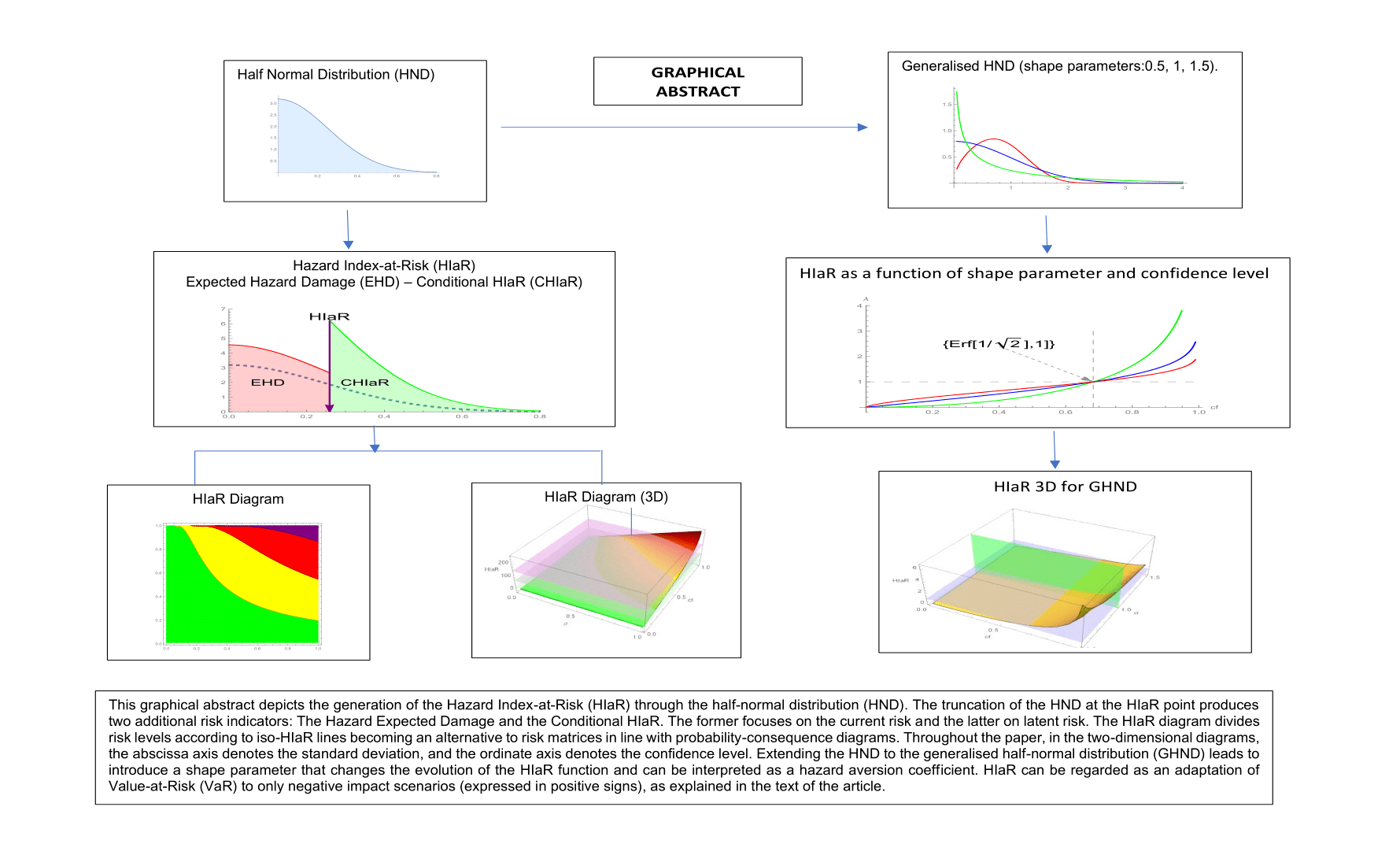Scheme 1 depicts these interactions.

Let us recall that VaR is defined as the maximum loss that an institution faces in the next period with a certain probability, p. This means, in other words, that the institution does not expect a higher loss than the VaR with probability 1 − p (confidence level). For the case of banks, the usual choice is 1% probability (i.e., 99% confidence level) for ten days. VaR is also used in corporate risk with longer horizons and lower confidence levels. A normal distribution of gains is the most usual in VaR calculations, although other distributions are also applied. This distribution includes gains and losses as negative gains ([25] p. 305). The TR model displays a setting where only negative impacts, namely losses, are possible. These losses consist of reductions in the safety index. To incorporate them into the TR model, we define the risk rate $\left(x\right)$ as the relative change in the initial value of the safety index produced by a hazard. The risk rate systematically expresses a reduction in the safety index. Losses are calculated as the product of the initial value of the safety index by the current value of the risk rate. Formally, the loss at the moment $t$ $\left(L_t\right)$ and the value of the safety index after this loss $\left(S{F}_t\right)$ are

$$L_t=S{F}_{t-1}{x}_t$$

(1)

$$S{F}_t=S{F}_{t-1}\left(1-x_t\right)$$

(2)

The TR model assumes that the risk rate follows a half-normal probability distribution because it can take only positive signs under the assumptions previously introduced. Since losses are expressed as the product between the constant initial value of the safety index and this rate, they follow a half-normal distribution as well. Appendix A summarises the main properties of the half-normal probability distribution used in this paper.

We define HIaR as the maximum potential reduction that the safety index can suffer in the next period with a probability equal to or lower than the maximum reasonable probability of the hazard occurrence. HIaR shares with VaR the property of being quantiles. Alexander ([26], p. 13) introduced VaR by writing “Value at risk is a loss that we are fairly sure that will not be exceeded if the current portfolio is held over some period of time”. Paralleling this definition, HIaR can be conceived as the hazards impact that the analyst is reasonably sure will not be exceeded.

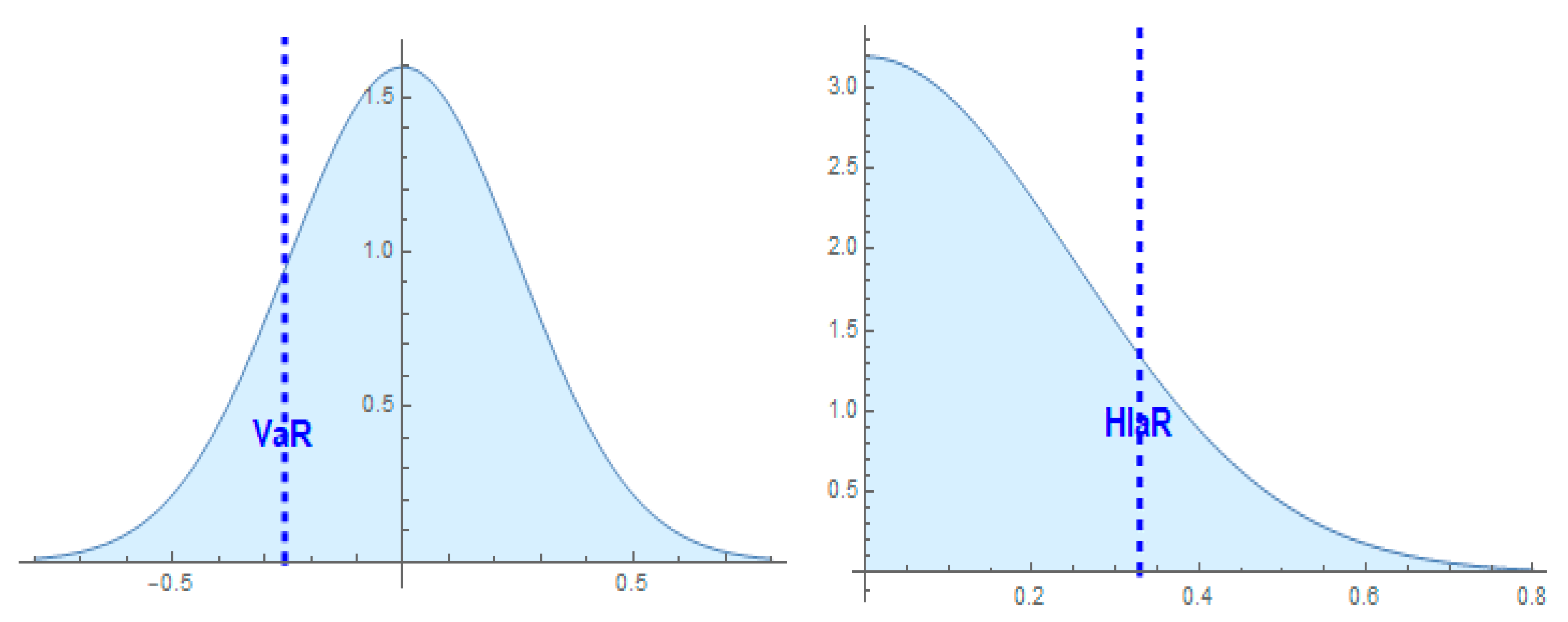
The comparison between the areas of corresponding probability distributions at the left-hand side and at the right-hand side of the quantiles (VaR and HIaR) clarify the meanings, especially the meaning of the confidence levels associated with VaR and HIaR. The area under the probability density function on the left-hand side of VaR expresses the probability of losing more than VaR. The area on the right-hand side of HIaR measures the probability of suffering damage greater than HIaR. Therefore, the corresponding confidence levels are referred to as opposite areas. As known, the confidence level for VaR is measured by the area on its right-hand side.

Conversely, the confidence level for HIaR is measured by the area on its left-hand side. Associating HIaR with the probability expected by the analyst, the area on its left-hand side expresses the maximum expected probability of the occurrence of the hazards. In contrast, the area on its right-hand side expresses the probability of experiencing damage greater than HIaR, i.e., it can be regarded as the surprise probability. For this reason, the probability of having damage equal to or lower than HIaR is a confidence level. Figure 1 represents the comparison between VaR and HIaR. The probability of facing damage greater than HIaR, which generates the CHIaR, is the centre of the analysis presented in Section 6.

Calculation of HIaR requires estimation of the standard deviation of the risk rate and deciding the confidence level. The standard deviation can indistinctively be referred to as the half-normal distribution or its equivalent value for the normal distribution due to the univocal relationship that exists between both (see Appendix A, Equation (A5)). The formulas that follow incorporate the standard deviation of the equivalent normal distribution. As known, the half-normal probability distribution function is as follows:

$$f\left(x\right)=\frac{1}{\sigma }\sqrt{\frac{2}{\pi }}{\mathrm{e}}^{-\frac{x^2}{2{\sigma }^2}}\mathrm{d}x$$

(3)

Designating by ${\gamma }_{\sigma ,cf}$ the value of risk rate $x$ that matches the standard deviation $\sigma$ and the confidence level $cf$, we can write the following:

$$\underset{0}{\overset{{\gamma }_{\sigma ,cf}}{\int }}\frac{1}{\sigma }\sqrt{\frac{2}{\pi }}{\mathrm{e}}^{-\frac{x^2}{2{\sigma }^2}}\mathrm{d}x=cf$$

(4)

Calculating this integral, we obtain

$$Erf\left[\frac{{\gamma }_{\sigma ,cf}}{\sqrt{2}\sigma }\right]=cf$$

(5)

and solve it for $\gamma$:

$${\gamma }_{\sigma ,cf}=\sigma \sqrt{2}Er{f}^{-1}\left[cf\right]$$

(6)

$Er{f}^{-1}\left[cf\right]$ stands for the inverse of the error function of the confidence level, i.e., the inverse of the following:

$$Erf\left[cf\right]=\frac{2}{\sqrt{\pi }}{\displaystyle \underset{0}{\overset{cf}{\int }}{e}^{-x^2}}dx$$

(7)

which is calculated through numerical methods.

At this point, HIaR is obtained straightforwardly by multiplying ${\gamma }_{\sigma ,cf}$ by the initial value of the safety index:

$$HIa{R}_{\sigma ,cf}=SF\cdot {\gamma }_{\sigma ,cf}$$

(8)

Since the notation ${\gamma }_{\sigma ,cf}$ stands for the risk rate that, once multiplied by the initial value of the safety index, generates HIaR, it can be the denominated HIaR rate.

In that the former refers to expected values while the latter expresses actual values. Comparing their dependent variables, $L$ stands for an actual loss whereas HIaR stands for an expected loss. It stems from Equation (6) that the expected value of the HIaR rate is proportional to the standard deviation. Thus, designating by ${\gamma }_{1,cf}$ the expected HIaR rate for standard deviation 1 and confidence level $cf$, we have the following:

$${\gamma }_{\sigma ,cf}=\sigma \cdot {\gamma }_{1,cf}$$

(9)

where

$${\gamma }_{1,cf}=\sqrt{2}\cdot Er{f}^{-1}\left[cf\right]$$

(10)

which is the value of $\gamma$ for $\sigma =1$ and the corresponding $cf$.

Thus, HIaR can be expressed as follows:

$$HIaR=SF\cdot \sigma \cdot {\gamma }_{1,cf}$$

(11)

Switching to the logarithmic scale in Equations (9) and (11), we can immediately separate the effects of the standard deviation and the confidence level.

The expression of the HIaR rate shown in (6) conveys that the HIaR rate turns out to be the product of two effects:

(a)

The severity effect $\sigma$ that associates the HIaR rate to the severity of the hazards impact.

(b)

The probability effect, $\sqrt{2\cdot }Er{f}^{-1}\left[cf\right]$, that expresses the influence of the confidence level on the HIaR rate because it can be interpreted as the normalised HIaR rate for $\sigma =1,$ i.e., ${\gamma }_{1,cf}$.

These effects parallel the traditional approach of risk matrices, where the impact size measures the severity effect and the estimated occurrence probability directly expresses the probability effect. In the TR model, both effects are filtered through the HIaR formula shown in Equation (6). Their product with the safety index in (11) simply means a change of scale. It stems from Equation (6) that the HIaR rate is proportional to the severity effect. Centring on the probability effect, we observe that it is a monotonously increasing function of $cf$ that approaches zero when $cf$ approaches zero as well. It equates 1 when $cf$ equates $Erf\left[1/\sqrt{2}\right]$ (0.6827 approximately) and approaches positive infinity when $cf$ approaches 1. Thus, the probability effect is lower than 1 for $cf$ between zero and $Erf\left[1/\sqrt{2}\right]$ and greater than 1 for probabilities between $Erf\left[1/\sqrt{2}\right]$ and 1. The consequence of these properties for the HIaR rate is that the probability effect reduces HiaR for probabilities lower than $Erf\left[1/\sqrt{2}\right]$ and increases this rate for probabilities higher than $Erf\left[1/\sqrt{2}\right]$.

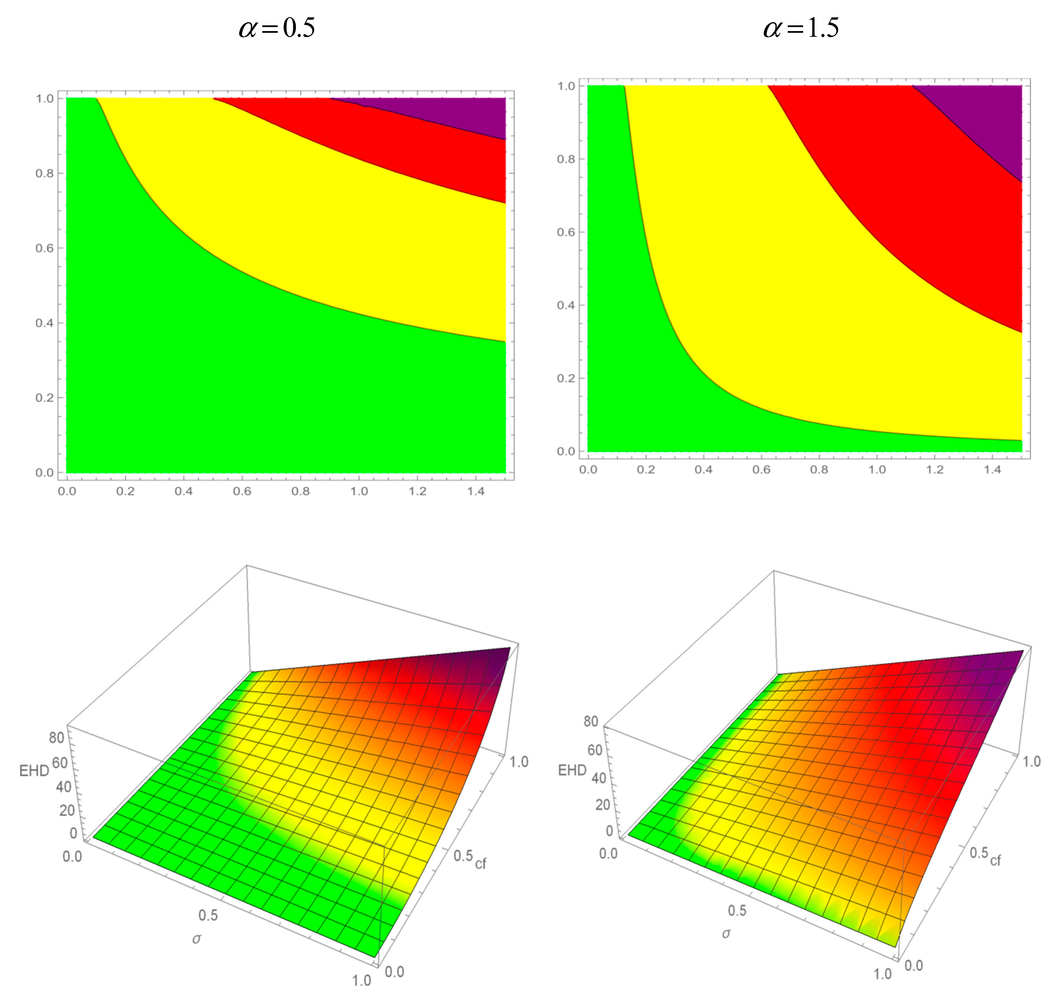
Figure 2 shows the evolution of HIaR as an increasing function of the standard deviation and the confidence level. The colours are scaled according to the traditional risk matrices convention: green for low risk, yellow for medium risk, and red for high risk, with added purple for very high risk. The right-hand-side plot includes a plane, denoted by grey lines, set up at 100 HIaR points to visualise the probability–severity combinations that express damage greater than the initial value of the safety index.

3. HIaR Diagrams vs. Risk Matrices

The conceptual centre of risk matrices consists of estimating the risk levels of the potential hazards under analysis by interacting the probability and severity of their impacts. Often, the numerical values of the probability and the impact level are outcomes of informed but subjective decision-makers’ criteria. The most common estimation of risk levels consists of the product between probability and severity. Next, the expected impacts are gathered into homogeneous categories that receive a similar treatment in the organization’s risk policy. The different risk categories are determined according to the values of probabilities and impacts that managers regard as appropriate for becoming boundaries between the risk categories. The horizontal and vertical boundaries generate the characteristic grid shape of risk matrices. Despite their intuitive appeal, risk matrices cannot achieve a complete homogeneous classification of risk levels as pointed out in the Introduction section. CPCDs are also based on the interaction between probability and severity. Frequently, CPCDs estimate risk levels as the product between both parameters. In this case, the difference between CPCDs and risk matrices consists of the different structures of their diagrams, although they share the same method for estimating risk levels. The HIaR diagrams built up in this section constitute a variant of CPCDs. Equal to CPCDs, HIaR diagrams divide risk zones through continuous iso-risk lines, now iso-HIaR lines. HIaR diagrams incorporate not only the intuition but also the rigour of VaR into CPCD analysis.

A central feature of risk matrices is their division in action zones denoted by different risk categories. In this respect, a risk category is constituted by the values of risk levels that deserve a similar course of action. Any risk matrix is divided at least into three action zones. Each zone recommends a different kind of action. For instance, “wait-and-see”, “short-term-management”, and “structural change”. The TR model replaces the rectangular delimitation of action zones used in risk matrices by introducing iso-HIaR lines as the boundaries of action zones. An iso-HIAR line consists of the combination of confidence levels and standard deviations that generate the same value of HIAR. Designating by $HIa{R}_j$ the constant value of HIaR that determines the iso-HIaR line $j$, by substituting in (11) HIaR by $HIa{R}_j$ and ${\gamma }_{1,cf}$ for its expression according to (10), we obtain the function that determines the pairs of $\sigma$ and $cf$ that generate the iso-HIaR line for $HIa{R}_j$.

Any HIaR diagram needs defining boundary Hia R levels, which become the boundaries that delimit the action zones. The HIaR rate $\left({\gamma }_{\sigma ,cf}\right)$ shown in (6) is proven to be a useful tool for deciding the boundaries of the HIaR diagram because it can be interpreted as the percentage that HIaR represents on the safety index, namely the percentage of the safety index that HIaR would destroy in the case of being real. Then, HIaR boundaries can be decided according to the HIaR rates that justify a change in the action zone, according to the analysts’ criteria. HIaR matrices may complement HIaR diagrams. A HIaR matrix consists of displaying in matrix form the HIaR values that match the chosen combinations of standard deviations, shown in the upper row, and the confidence levels shown in the left-hand-side column. Due to this discrete structure, a HIaR matrix is not appropriate for separating iso-risk zones.

Table 1. HIaR matrix.

	σ	0.01	0.05	0.25	0.5	0.75	1	1.5
cf
0.99		2.58	12.88	64.40	128.80	193.20	257.60	386.40
0.95		1.96	9.80	49.00	98.00	147.00	196.00	294.00
0.75		1.15	5.75	28.76	57.52	86.28	115.00	172.60
0.5		0.67	3.37	16.86	33.72	50.59	67.45	101.20
0.25		0.32	1.59	7.97	15.93	23.90	31.86	47.80
0.05		0.06	0.31	1.57	3.14	4.70	6.27	9.41
0.01		0.01	0.06	0.31	0.63	0.94	1.25	1.88

Table 1 shows the values of HIaR for the given values of the standard deviation and confidence levels.

shows the HIaR matrix for the given standard deviations and confidence levels. These HIaR values can be interpreted as percentages. For instance, for a standard deviation of 0.25 (severity) and a confidence level (probability) of 0.25, the expected damage in the safety index is 7.97%. However, if severity equates 0.75 and probability equates 0.95, then the expected damage goes beyond the current value of the safety index (100 points) reaching 147% of it, which means that the damage exceeds 47% of the value embedded in the safety index. At the same time, the first column shows the probability effect, i.e., ${\gamma }_1$.

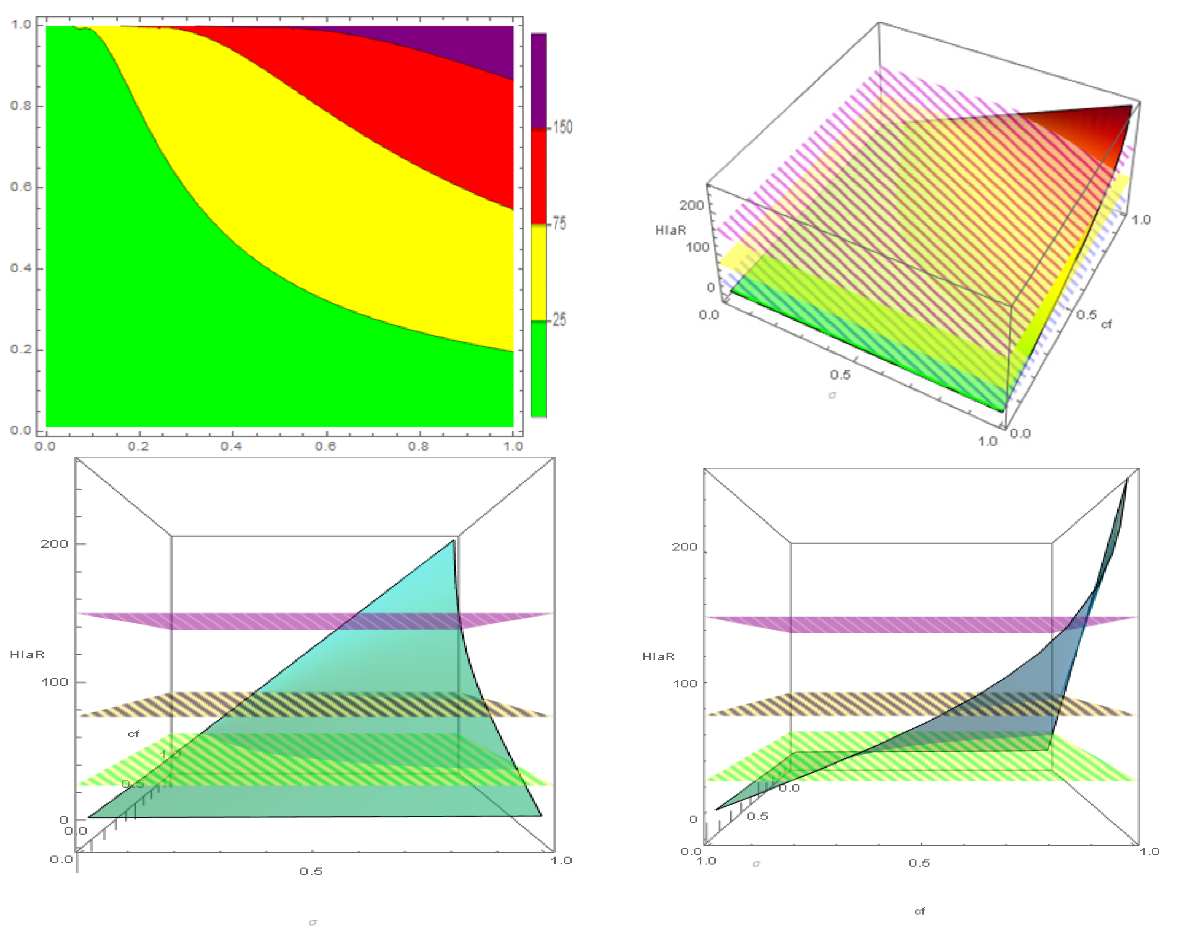
Figure 3 shows the HIaR diagram as a two-dimensional plot and three three-dimensional plots. Their data are the same as that generated by the HIaR matrix in Table 1. As Figure 2 and Figure 3 include four risk levels denoted by green (low risk), yellow (medium risk), red (high risk), and purple (extreme risk) colours. The boundary levels are set up at 25 points for starting the yellow level, 75 for starting the red level, and 150 for starting the purple level. The three three-dimensional plots display the figure from three different points of view on behalf of clarity. In them, iso-HiaR planes have substituted iso-HiaR lines. Throughout the paper, in the two-dimensional diagrams, the abscissa axis denotes the standard deviation and the ordinate axis denotes the confidence level.

4. The Expected Hazards Damage

HIaR would become incomplete without connecting it to the expected loss in case of a hazard taking place. We define the Expected Hazards Damage (EHD) as the expected loss due to the risk under analysis, i.e., the expected loss if the hazard becomes real. Recalling that HIaR expresses maximum loss in the safety index (SF) under the estimated probability $cf$, the EHD can be written as follows:

$$EHD=\frac{1}{cf}SF\underset{0}{\overset{{\gamma }_{\sigma ,cf}}{{\displaystyle \int }}}\frac{1}{\sigma }x\sqrt{\frac{2}{\pi }}{\mathrm{e}}^{-\frac{x^2}{2{\sigma }^2}}\mathrm{d}x$$

(12)

where $1/cf$ adjusts the probability of the half-normal distribution to the area between zero and $cf$.

Solving the integral in Equation (12), we obtain the following:

$$EHD=SF\frac{1}{cf}\left(1-{\mathrm{e}}^{-Er{f}^{-1}{\left[cf\right]}^2}\right)\sqrt{\frac{2}{\pi }}\sigma$$

(13)

Paralleling the breaking down of the HIaR between the probability effect and the severity effect, this equation extends this decomposition to EHD. Now, $\sigma$ continues being the severity effect, while $\frac{1}{cf}\left(1-{\mathrm{e}}^{-Er{f}^{-1}{\left[cf\right]}^2}\right)\sqrt{\frac{2}{\pi }}$ becomes the probability effect.

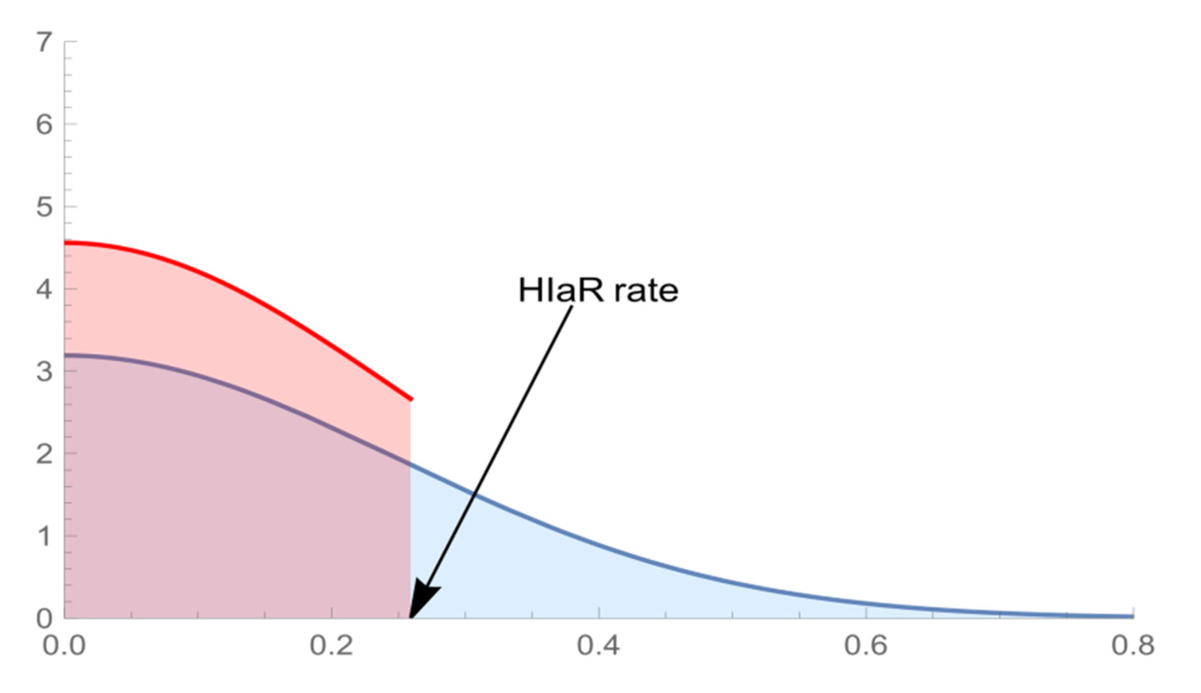
It stems from Equation (12) that EHD consists of the mathematical expectation of the probability distribution of the hazards impacts that do not exceed the maximum expected impact, i.e., do not exceed HIaR. Thus, this distribution is a half-normal truncated at the HIaR point. Equation (12) shows this property by truncating the half-normal distribution of the risk rate $x$ at the HIaR rate ${\gamma }_{\sigma ,cf}$. 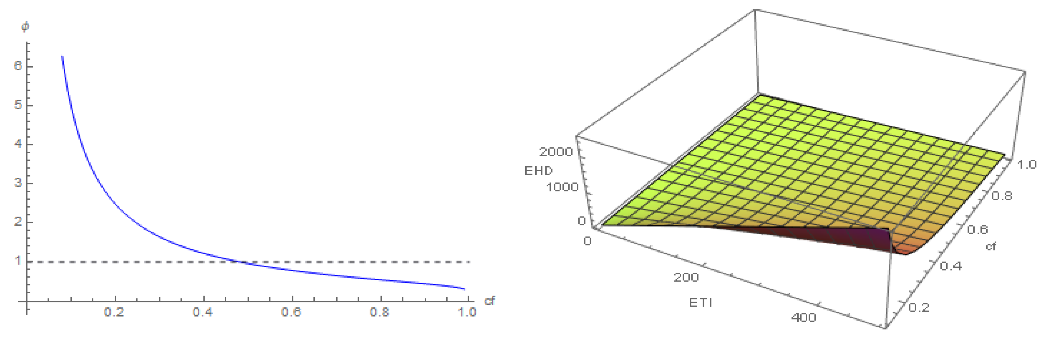Figure 4 illustrates this property. The left-hand side of Figure 5 shows the EHD plot expressing EHD as a function of $\sigma$ and $cf$. Its right-hand side shows the EHD diagrams.

EHD can be expressed as a function of HIaR, which clarifies the relationship between both. Solving (11) for $\sigma$ and substituting ${\gamma }_{1,cf}$ according to (10), we obtain

$$\sigma =\frac{HIaR}{SF\sqrt{2}\cdot Er{f}^{-1}\left[cf\right]}\cdot$$

(14)

and substituting (14) into (13), we obtain

$$EHD=\frac{\left(1-{\mathrm{e}}^{-Er{f}^{-1}{\left[cf\right]}^2}\right)}{\sqrt{\pi }cf\cdot Er{f}^{-1}\left[cf\right]}HIaR$$

(15)

which shows that the relationship between EHD and HIaR is ruled by the function of the HIaR–EHD connector $(\vartheta )$:

$$\vartheta =\frac{\left(1-{\mathrm{e}}^{-Er{f}^{-1}{\left[cf\right]}^2}\right)}{\sqrt{\pi }cf\cdot Er{f}^{-1}\left[cf\right]}$$

(16)

that has the confidence level as the unique independent variable. Figure 6 illustrates the relationship between EHD and HIaR.

5. The Expected Hazards Damage vs. Traditional Risk Matrices Approach

Analysing the traditional risk matrices approach from EHD reveals hidden information of the hazard under analysis. The traditional approach obtains the expected impact through the product between the estimated probability and the size of the impact. Henceforth, we will call this product Expected Traditional Impact (ETI):

$$ETI=p\cdot IS$$

(17)

where p stands for probability and IS stands for impact size.

Both ETI and EHD share being expected values. The difference between them lies in the obtainment processes. The calculation of EHD substitutes the direct product between probability and impact size shown in (17) by expression (13), where the expected value of the half-normal distribution between zero and the HIaR rate is adjusted according to the confidence level. The relationship between ETI and EHD can be explored analytically. The algorithm we present next transforms ETI in EHD, revealing hidden information in the former. The algorithm proceeds as follows:

(1)

The probability and the impact size are accepted as data to obtain ETI according to (17).

(2)

The probability is assimilated to the confidence level $\left(p=cf\right)$.

(3)

The impact size is assimilated to HIAR $(IS=HIaR)$.

(4)

From the confidence level and HIaR, we obtain the standard deviation embedded in the impact size (IS) through Equation (14) by substituting HIaR for IS. The knowledge on this standard deviation is not necessary for relating ETI with EHD, but it can be compared with historical and estimated volatilities to evaluate the soundness of the ETI calculated through the traditional method.

(5)

Having assimilated IS to HIaR, it stems from (17) that HIaR can be equated to the ratio between ETI and cf because cf substitutes p in the TR model.

(6)

Substituting HIaR in (15) by the quotient between ETI and cf, we obtain the relationship between ETI and EHD:

$$EHD=\frac{\left(1-{\mathrm{e}}^{-Er{f}^{-1}{\left[cf\right]}^2}\right)}{\sqrt{\pi }c{f}^{2}Er{f}^{-1}\left[cf\right]}ETI$$

(18)

Thus, the function that links EHD with ETI is as follows:

$$\varphi =\frac{\left(1-{\mathrm{e}}^{-Er{f}^{-1}{\left[cf\right]}^2}\right)}{\sqrt{\pi }c{f}^{2}Er{f}^{-1}\left[cf\right]}$$

(19)

Figure 7 illustrates the relationship between EHD and ETI.

6. On Active and Latent Risks: Conditional HIaR

This section delves into the comparative analysis between the maximum expected probability and the surprise probability introduced in Section 2 when considering damage greater than HIaR. The evolution from the HIAR to the analysis of the expected values associated with it requires precise interpretation of the probability that determines the HIaR, henceforth, the HIaR probability. The binary approach of traditional risk matrices incorporates two probabilities exclusively: the one associated with the occurrence of the hazard and the one that discards the idea that the hazard will take place. In contrast, this paper centres its analysis on a continuous distribution, the half-normal. Obtaining HIaR through the half-normal distribution reveals the existence of three relevant levels of the expected value: the total potential risk, the expected active risk, and the latent risk.

The total potential risk consists of the expected value that stems from the whole probability distribution. Thus, it consists of the mathematical expectation of the potential hazard that the risk under analysis may generate. However, not necessarily, the entire potential risk constitutes an active threat. One part of it may be active, and the rest may be latent. The central feature of the latent part of the risk is that, under the current circumstances, it does not show any sign that it will produce any hazard on the horizon of the analysis. The expected active risk consists of the expected value of hazards that goes from zero to the HIaR probability, i.e., from a null probability to its maximum expected value. Finally, the latent risk is the expected value of the latent part of risk placed on the right-hand side of the HIaR probability. This latent risk is congruent with the risk associated with CVaR and placed on the left-hand side of VaR.

The previous analysis has focused on the area between the origin and the confidence level of the half-normal distribution. The whole area of distribution and the area on the right-hand side of the confidence level complement its information. The total area under distribution can be interpreted as the total mathematical expectation (TME) of a hazard with volatility of the case under analysis. For the half-normal distribution, the unique variable of this area is the standard deviation:

$$TME=S{F}_0\underset{0}{\overset{\infty }{{\displaystyle \int }}}\frac{1}{\sigma }x\sqrt{\frac{2}{\pi }}{\mathrm{e}}^{-\frac{x^2}{2{\sigma }^2}}\mathrm{d}x$$

(20)

Solving the integral in Equation (20), we obtain the following:

$$TME=S{F}_0\sqrt{\frac{2}{\pi }}\sigma$$

(21)

Since $\sqrt{2/\pi }$ is equal to 0.7979, the TME approximately equates to 80% of the standard deviation multiplied by the initial value of the index.

The right-hand-side area expresses the discarded impact, more specifically, the impact that analysts estimate that will not take place and, for this reason, discard it from the study. Paralleling EHD, the expected value on the right-hand side of the distribution leads to the Conditional HiaR (CHIaR), which means the potential impact excluded from the analysis:

$$CHIaR=S{F}_0\frac{1}{1-cf}\underset{{\gamma }_{\sigma ,cf}}{\overset{\infty }{{\displaystyle \int }}}\frac{1}{\sigma }x\sqrt{\frac{2}{\pi }}{\mathrm{e}}^{-\frac{x^2}{2{\sigma }^2}}\mathrm{d}x$$

(22)

Solving the integral in Equation (22), we obtain the following:

$$CHIaR=S{F}_0\frac{1}{1-cf}{\mathrm{e}}^{-Er{f}^{-1}{\left[cf\right]}^2}\sqrt{\frac{2}{\pi }}\sigma$$

(23)

CHIaR can be regarded as the source of unexpected hazards known as black swans. CHIaR has a parallel meaning with CVaR because the former focuses on damage when the HIaR barrier is crossed and the latter focuses on losses when the VaR barrier is crossed.

TME, EHD, and CHIaR fulfil the following properties: when the confidence level approaches 1, EHD approaches TME and CHIaR approaches zero. TME, in turn, is the weighted average of EHD and CHIaR with $cf$ and $\left(1-cf\right)$ as weighting coefficients.

$$\underset{cf\to 1}{\lim }EHD=TME$$

(24)

$$\underset{cf\to 1}{\lim }CHIaR=0$$

(25)

$$cf\cdot EHD+(1-cf)\cdot CHIaR=TME$$

(26)

Figure 8 displays the probability distributions of total risk, active risk, and latent risk.

7. A Subjective Approach to Risk Analysis through the Half-Normal Distribution

The relevant contribution of subjective probabilities to decision-making reasoning is widely acknowledged. Their use in risk analysis is part of this contribution as well. Karni [29] systematised their axiomatic foundations. Andersen et al. [30] studied the joint estimation of subjective probabilities and risk attitudes. Wintle et al. [31] dealt with the numerical translation of verbal probabilities. Aven and Reiners [32] presented an in-depth analysis of the interpretation of probabilities in risk analysis with particular emphasis on the meaning and use of subjective probabilities. Goerlandt and Reiners [33] applied subjective probabilities to probability–consequence diagrams. Flage et al. [34] developed a critical perspective on the use of subjective probabilities in risk analysis, showing how incorporating probability bounds may improve the performance of the analysis. Langdalen et al. [35] dealt with the identification of hidden assumptions in risk studies focusing on the subjective nature of risk assessment.

This section aims to show how the analytical framework created by the TR model can be used also as a tool for subjective reasoning in risk analysis. In this way, generic risk perceptions can be turned into a set of linked variables, the coherence of which can be discussed through the lenses of the logic relationships embedded in the model. In concrete, this section presents an algorithm that, departing from subjective assumptions of the maximum downwards associated with the total risk and the active risk, delivers the values of the standard deviation, the confidence level, and the HIaR embedded in the assumed downwards. The algorithm proceeds as follows:

(1)

The hypothesis for the maximum downward coefficient of total risk leads to obtainment of the standard deviation by applying a property of binomial trees. In effect, binomial trees used in option pricing (Cox, Ross, and Rubinstein [36]) relate in approximate terms the upward and downward coefficients with the standard deviation. For the downward coefficient $\left(d\right)$, the relationship for one-time period is as follows:

$$e^{-\sigma }=d$$

(27)

Based on this relationship, the analyst may obtain the standard deviation after estimating the maximum downward that s/he may expect in the safety index. This estimation includes the active and the latent risk, i.e., it refers to the total risk.

(2)

By introducing a hypothesis for the maximum downward coefficient of the active risk $\left(d^{\prime }\right),$ the analyst identifies the subjective HIaR embedded in this downward coefficient. Since HIaR represents the maximum expected reduction in the safety index, the relationship between $d^{\prime }$, $SF$, and $HIaR$ is

$$SF\cdot (1-d^{\prime })=HIaR$$

(28)

(3)

To unveil the confidence level that stems from the obtained values of HIaR and the standard deviation, we calculate, first, the value of the HIaR rate $\left({\gamma }_{1,cf}\right)$ from Equation (11). Next, substituting it into Equation (10), we obtain the confidence level.

Summarising, through subjective estimations of the downward coefficients for the total risk and the active risk ($d$ and $d^{\prime }$), the analyst obtains the set $\left\{\sigma ,HIaR,cf\right\}$ and starts revising its coherence from his/her criteria and the information available for similar settings. The aim of this algorithm is not to substitute an in-depth analysis of subjective reasoning but to provide a first approach to turning subjective perceptions into a quantitative setting in a straightforward manner grounded on analytical tools. Scheme 2 presents a conceptual map of this algorithm.

8. Exploring the Generalised Half-Normal Distribution

Many probability distributions have been applied to risk analysis. Although this paper has centred on the half-normal distribution, the essence of its methodological proposition has consisted of developing CPCDs through a right-truncated probability distribution applied on a hazards rate. The half-normal distribution brings the advantage of depending only on its scale parameter ($\sigma$), but at the same time, this property limits its capacity for studying scenarios that would be better modelled by changing the shape of the distribution. The generalised half-normal distribution (GHN), proposed by Cooray and Ananda [11], incorporates a shape parameter to the original half-normal distribution, adding flexibility to its analytical capacity. This section explores the main changes that switching from the half-normal to its generalised counterpart produces on the previous results of this paper, focusing on HIaR mainly. The probability density function of the generalised half-normal distribution ([11], p. 1125) is as follows:

$$GHN=\sqrt{\frac{2}{\pi }}\left(\frac{\alpha }{x}\right){\left(\frac{x}{\sigma }\right)}^{\alpha }{\mathrm{e}}^{-\frac{1}{2}{\left(\frac{x}{\sigma }\right)}^{2\alpha }}$$

(29)

if $x>0$ and 0 otherwise.

In (29), $\alpha$ stands for the shape parameter and $\sigma$ stands for the location parameter, substituting the Greek letter theta $\left(\theta \right)$ used by Cooray and Ananda on behalf of homogeneity with the half-normal distribution notations previously used in this paper and in other papers quoted in the Section 1 and in the Appendix. The properties of the generalised half-normal distribution, including its statistical moments, are presented by Cooray and Ananda [11].

Next, we focus on the applicability of the generalised half-normal to HIaR. The basic results for EHD are presented in Appendix B. The HIaR rate for the generalised half-normal $\left(\lambda \right)$ fulfils the following condition:

$$\underset{0}{\overset{\lambda }{\int }}\frac{{\mathrm{e}}^{-\frac{1}{2}{\left(\frac{x}{\sigma }\right)}^{2\alpha }}\sqrt{\frac{2}{\pi }}\alpha {\left(\frac{x}{\sigma }\right)}^{\alpha }}{x}\mathrm{d}x=cf$$

(30)

which parallels (4) for the original half-normal. Calculating this integral and solving it for $\lambda$, we obtain the values of the HIaR rate for $\sigma$, $cf$, and $\alpha$:

$$\lambda =\sigma {\left(\sqrt{2}\cdot Er{f}^{-1}\left[cf\right]\right)}^{\frac{1}{\alpha }}$$

(31)

Taking (10) into account, this equation can be written as follows:

$$\lambda =\sigma \cdot {\gamma }_{1,cf}^{\frac{1}{\alpha }}$$

(32)

As for the notations, $\lambda$ denotes the generalised HIaR rate for the generalised half-normal distribution, henceforth generalised HIaR rate, while $\gamma$ continues designating the same rate for the ordinary half-normal distribution. Both rates become equal for $\alpha =1$ (Pescim et al. [12], p. 946). The parameters $\sigma$, $cf$, and $\alpha$ remain implicit in $\lambda$, the complete notation of which would be ${\lambda }_{\sigma ,cf,\alpha }$.

The generalised HIaR rate, as its ordinary counterpart, embeds the severity effect and the probability effect. The former $\left(\sigma \right)$ remains unchanged. The latter equates the HIaR rate for $\sigma =1$ powered at the inverse of the shape parameter $\alpha$. The comparison between the probability effects of the generalised and the ordinary half-normal distribution explains the changes that the shape parameter introduces in the generalised HIaR rate.

Table 2. Comparing the probability effects (${\lambda }_1$ vs. ${\gamma }_1$).

	$0<\mathit{c}\mathit{f}<\mathit{E}\mathit{r}\mathit{f}\left[1/\sqrt{2}\right]$ ${\mathit{\gamma }}_{1,\mathit{c}\mathit{f}}<1$	$\mathit{c}\mathit{f}=\mathit{E}\mathit{r}\mathit{f}\left[1/\sqrt{2}\right]$ ${\mathit{\gamma }}_{1,\mathit{c}\mathit{f}}=1$	$\mathit{c}\mathit{f}>\mathit{E}\mathit{r}\mathit{f}\left[1/\sqrt{2}\right]$ ${\mathit{\gamma }}_{1,\mathit{c}\mathit{f}}>1$
$\alpha <1$	$\lambda <\gamma$	$\lambda =\gamma =1$	$\lambda >\gamma$
$\alpha =1$	$\lambda =\gamma$	$\lambda =\gamma =1$	$\lambda =\gamma$
$\alpha >1$	$\lambda >\gamma$	$\lambda =\gamma =1$	$\lambda <\gamma$
Region plot: the blue zones denote $\lambda <\gamma$, and the white zones denote $\lambda >\gamma$.

Table 2 compares HIaR rates for the half-normal distribution $\left(\gamma \right)$ and the generalised half-normal distribution $\left(\lambda \right)$. Since both are directly proportional to the severity effect $\left(\sigma \right)$, comparing $\lambda$ and $\gamma$ is equivalent to comparing ${\lambda }_{1,cf,\alpha }$ and ${\gamma }_{1,cf}$. The region plot, built through the Mathematica software, highlights in blue the zones in which ${\lambda }_1<{\gamma }_1$ and in white the zones that fulfil ${\lambda }_1>{\gamma }_1$.

summarises these changes. The first step of this comparison consists of realising that a confidence level, $cf$, equal to $Erf\left[1/\sqrt{2}\right]$ (0.6827 approximately) neutralises the $\alpha$ impact because it equates ${\gamma }_{1,cf}$ to 1. When $cf<Erf\left[1/\sqrt[]{2}\right]$ and, thus, ${\gamma }_1<1$, a shape parameter lower than 1 increases the probability effect, while $cf>Erf\left[1/\sqrt[]{2}\right]$ increases it because now we have ${\gamma }_1>1$. The effects for $cf>Erf\left[1/\sqrt{2}\right]$ are the opposite.

The study of the ratio between the HIaR rates for the generalised and the ordinary half-normal distribution, henceforth denoted by $\varsigma$, enlightens the role of the shape parameter. The expression of this ratio is as follows:

$$\varsigma =\frac{\lambda }{\gamma }={\left(\sqrt{2}\cdot Er{f}^{-1}\left[cf\right]\right)}^{\left(\frac{1}{\alpha }-1\right)}$$

(33)

which, in turn, consists of the ratio of both probability effects, that, recalling (10) and (32), can be written as follows:

$$\varsigma ={\gamma }_{1,cf}^{\left(\frac{1}{\alpha }-1\right)}$$

(34)

Thus, $\left(\varsigma -1\right)$ expresses the percentage in which $\alpha$ changes the probability effect and, at the same time, the HIaR rate. Interestingly, high $\alpha$ values compensate the low probability effect associated with very low probabilities. Often, academic papers on risk analysis have pointed out that scenarios with high severity and low probability should be rated riskier than scenarios with lower severity and higher probability that present the same value of the risk indicator. In this respect, Duijim [21] (p. 27) defined the hazard aversion as “the attitude that a low probability-large consequence event is assigned a higher risk value than a high probability-low consequence event, even when the expected loss for both events is the same”. The capacity of the shape parameter of the generalised half-normal distribution for weighting the probability effect opens the way for increasing its impact of HIaR and EHD in case of low probabilities by assigning to the shape parameter the function of a hazard aversion coefficient in the case of low probabilities and high impacts. The development of this topic needs further research.

Table 3. HIaR rates ratio $\left(\lambda /\gamma \right)$.

	$\mathit{\alpha }$	0.1	0.5	1	1.5	2
cf
0.05		0.0000	0.0627	1	2.5171	3.9934
0.5		0.0289	0.6745	1	1.1403	1.2176
0.6827		1	1	1	1	1
0.75		3.5275	1.1503	1	0.9544	0.9324
0.99		4991.76	2.5758	1	0.7295	0.6231

Table 3 displays the values of the HIaR rates ratio for the given values of the shape parameter ($\alpha$) and the confidence level (cf).

displays the values of $\varsigma$ for different values of $\alpha$ (columns) and $cf$ (rows). Among other data, it shows that, for a 5% probability (cf), $\alpha$ equal to 2 increases the probability effect and the HIaR ratio at the same time, multiplying it by 3.993.

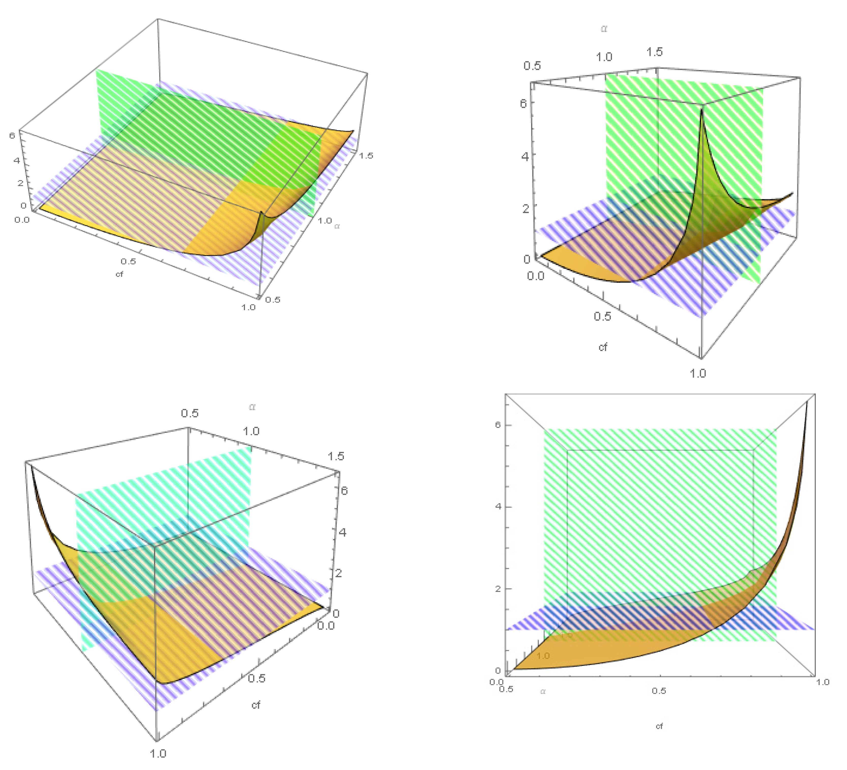
Figure 9 represents the evolution of the generalised HIaR ratio for $\sigma =1$, which is, at the same time, the evolution of the probability effect for the generalised HIaR ratio. The vertical plane is set up at $\alpha =1$, while the horizontal plane is set up at $cf=Erf\left[1/\sqrt{2}\right]$ (0.6827). The intersection between ${\lambda }_1$ (yellow surface) and the vertical plane shows the line of ${\gamma }_1$ because, as stated, ${\lambda }_1$ equates ${\gamma }_1$ for $\alpha =1$. The crossing between ${\lambda }_1$ and the horizontal plane shows how ${\lambda }_1$ evolves from values lower than 1 to values higher than 1 because $cf=Erf\left[1/\sqrt{2}\right]$ equates both ${\gamma }_1$ and ${\lambda }_1$ to 1.

Beyond these applications, the generalised half-normal distribution offers an interesting potential for its use in the analysis of VaR, CVaR, and CPCDs when fat tails and skew become a central point in the analysis, paralleling the developments of the generalised normal distribution made, among others, by Stoyanov et al. [37] and Chen et al. [38].

9. Discussion

Truncated probability distributions embed the essential features for analysing risky scenarios that may produce only negative impacts on the assets related to them. Among these distributions, the half-normal turns out to be the straightforward option for adapting VaR and CVaR to the probability–severity risk analysis performed through CPCDs, which overcome the misclassifications due to the rectangular structure of risk matrices. In effect, the iso-risk lines that separate the risk categories in CPCDs open the way for expressing them through risk indicators based on VaR and CVaR. Switching from the product between probability and severity to VaR and CVaR heightens the information level generated by the analysis. At the same time, it requires adapting VaR and CVaR to a setting characterised by truncated probability distributions. We have called the Truncated Risk (TR) model the outcome of adapting VaR and CVaR to CPCDs.

The methodology of the TR model has departed from defining the safety index and the hazards index analysed through the half-normal distribution. The former is referred to as a generic asset and represents the percentage of not being damaged by hazards. The latter expresses the impact of hazards on the safety index. Since the hazards index only captures negative impacts, although expressed in a positive sign, its random behaviour must be expressed through a truncated probability distribution. In this paper, we have opted for the half-normal distribution as the most straightforward issue. As a risk analysis tool, the half-normal distribution shows the advantage of depending on its standard deviation exclusively, namely, its scale parameter. Thus, for any risk setting that can be represented by a half-normal distribution reasonably, the standard deviation can be taken as an indicator of the severity of hazards. The probability of each hazard is now expressed through the maximum expected probability of the hazard occurrence, which turns out to be the confidence level associated with this probability. As a logical outcome, the probability on the right-hand side of the expected one becomes the surprise probability. It is, in other words, the probability that, in subjective terms, expresses the degree of the analyst believing that the hazard will not take place. The generalised half-normal distribution amplifies the analysis by including a shape parameter that adds flexibility to the model.

As shown, the two central risk indicators of the TR model, HIaR and EHD, can be interpreted as the product between a probability effect and a severity effect. Thus, they hold the original message of risk matrices. The comparison between both approaches enlightens the changes in the probability–severity analysis proposed in this paper. Instead of obtaining the estimated total impact (ETI) as a direct product between probability (p) and impact severity (IS), the TR model filters the information through the half-normal distribution. Now, this distribution embeds all possible impacts and their probabilities. The volatility drives the severity of the impacts because it determines the shape of the half-normal distribution. The probability of the traditional approach is replaced by the confidence level or the half-normal distribution. The HIaR shares with the traditional impact size (IS) the fact of expressing the maximum damage expected by the analyst because it expresses the maximum expected impact under the maximum expected probability. The primary difference between the traditional impact size and HIaR lies in the fact that the traditional impact size is a unique value associated with the hazard in any circumstance in which the hazard becomes real. At the same time, HIaR is based on a probability distribution, not necessarily the half-normal.

EHD is the concept that replaces the traditional total expected impact. In this way, the analysis gains flexibility because the single value of the estimated impact is now replaced by a tripled of values, which includes the total possible mathematical expectation (TME), the EHD, and its complement: the CHIaR. Thus, this approach induces decision-makers to make plans to face not only the expected (HIaR and EHD) but also the unexpected through CHIaR. As a clarification, it is worth pointing out that EHD does not have an equivalent measure in the framework of VaR analysis. HIaR parallels VaR, while CHIaR parallels CVaR, but the mathematical expectation of potential losses lower than VaR is not a standard risk indicator in financial analysis. Nevertheless, in the context of risk analysis through the half-normal distribution, EHD has become central for linking the VaR analysis developed in this paper with the traditional probability–severity approach of risk matrices.

Section 7 has presented a subjective, although analytical, approach to the TR model that stresses its side as a thinking tool for enabling analysts to find the risk parameters hidden on their subjective expectations on downside risk. The extension of the analysis to the generalised half-normal distribution has shown the property of the shape coefficient in modifying the probability effect increasing the weight of lower probabilities and decreasing the weight of the higher ones or in producing the opposite effect, depending on the choice of the shape parameter. The properties of the shape parameter justify interpreting it as the hazard aversion coefficient. Risk aversion and hazard aversion are different indicators: the former determines the required risk premium, while the latter rules by assigning risk levels in the combinations of the probability and severity of different hazards. It is, in particular, relevant for assigning higher risk levels to hazards of high impact and low probability when they are compared with low impact and high probability hazards. Besides, the introduction of the generalised half-normal distribution has shown how the TR model can be adapted to a truncated probability distribution different from the half-normal that has guided its development.

This paper has the limitation of having centred the analysis in the half-normal distribution. Its extension to the generalised half-normal has shown how more complex probability distributions may incorporate additional features than the ones of the half-normal. The risk measures that this paper has adapted to the probability–severity analysis, VaR and CVaR, have been extended also in the financial mathematics literature from the normal distribution to other probability distributions that may fit better to specific cases, fat tails in particular. These extensions take also into account the limitations of VaR in the face of subadditivity. In addition, interweaving the point of view of truncated distributions with some of the advances in risk management mentioned in the Introduction section, such as considering the knowledge dimension of risk, may contribute as well to widening the scope of the analysis presented in this paper.

10. Conclusions

By applying the half-normal distribution as its primary methodological tool, this paper has adapted VaR and CVaR to probability–severity risk analysis by building up a model that we have called the Truncated Risk (TR) model. The two central risk indicators proposed, HIaR and EHD, can be broken down into a severity effect that consists of the risk rate volatility and a probability effect that has the confidence level as its unique independent variable. Both indicators have been related functionally to compare and strengthen their meanings. The EHD truncates at the HIaR point the half-normal distribution that stems from the severity effect expressed by the risk rate volatility, which is, at the same time, the location parameter of the distribution. The part of the half-normal distribution not absorbed by the EHD, i.e., the one on the right-hand side of HIaR, can be interpreted as the unexpected hazards impact, which means the expected hazards damage embedded in the severity parameter but excluded by the estimation of the maximum probability of the hazard occurrence, namely, the confidence level, in the TR model. The division of the total mathematical expectation generated by the severity coefficient between EHD and CHIaR may help to consider surprises in addition to expectations in risk analysis. A simplified model, based on subjective probabilities, shows how the TR model may contribute to turning generic risk appreciations into a set of related parameters, the coherence of which can be revised by decision-makers to improve the outcomes of subjective appreciations.

The extension of the TR model to the generalised half-normal distribution has shown how incorporating a shape parameter enlarges the analytical capacity of the original approach. However, the most relevant conclusion of the extension to the generalised half-normal distribution has been to realise how the basic TR model can be broadened by introducing other truncated probability distributions that may fit better with the scenarios under analysis. Scheme A1 summarises the contents of this paper in a conceptual map.