Article

Topology Optimization of Elastoplastic Behavior Conditions by Selectively Suppressing Plastic Work

1
School of Mechanical Engineering, Sungkyunkwan University, Suwon, Gyeonggi-do 16419, Korea
2
Department of Smart Fab. Technology, Sungkyunkwan University, Suwon, Gyeonggi-do 16419, Korea
*
Author to whom correspondence should be addressed.
Mathematics 2020, 8(11), 2062; https://doi.org/10.3390/math8112062
Submission received: 10 October 2020 / Revised: 10 November 2020 / Accepted: 18 November 2020 / Published: 19 November 2020
(This article belongs to the Special Issue Applied Mathematics and Solid Mechanics)

Abstract

:
This work conducted topology optimization with an implicit analysis of elastoplastic constitutive equation in order to design supporting structures for unexpected heavy loading conditions. In this topology optimization model, plastic work was extracted from strain energy and selectively employed in the objective function according to deformation mode. While strain energy was minimized in elastic deformation areas, in elastoplastic deformation areas, the plastic work was minimized for the purpose of suppressing plastic deformation. This method can focus on suppressing plastic strain in the plastic deformation zone with maintaining elastic stiffness in the elastic deformation zone. These formulations were implemented into MATLAB and applied to three optimization problems. The elastoplastic optimization results were compared to pure elastic design results. The comparison showed that structures designed with accounting for plastic deformation had a reinforced area where plastic deformation occurs. Finally, a finite element analysis was conducted to compare the mechanical performances of structures with respect to the design method.

1. Introduction

Topology optimization is a scheme used to obtain a design with an optimized shape for a specific purpose, and is widely used in engineering problems [1,2,3,4,5,6,7,8,9,10,11]. The principle of topology optimization is to find an optimal distribution of material density within a design domain under constraint conditions. In structure design problems, strain energy is the first priority to be the objective function since minimizing strain energy can give a structure with a maximum stiffness. Under elastic deformation, calculating the strain energy is simple since stress and strain have a simple linear relation. In contrast, when a part of a material undergoes elastoplastic deformation, its material properties change according to the level of plastic strain, resulting in a nonlinear relation between stress and strain. This nonlinear relation leads to difficulties when attempting to determine stress and the material property matrix. Because of this, the majority of topology optimization applications are based on the assumption of elastic deformation [12,13,14,15,16,17,18]. Only a few researchers have tried to consider plastic deformation in topology optimization. Zhang et al. [19] employed enhanced assumed strain (EAS) elements to solve the locking issue, and Wallin et al. [20] made a multiplicative split of the deformation gradient. Schwarz et al. [21] conducted topology optimization for elastoplastic material by maximizing ductility. Blachowski et al. [22] recently proposed a stress intensity-driven elastoplastic topology optimization method to find a minimum weight structure that is able to carry a given load. Herfelt et al., [23] conducted a strength-based optimization resulting in a convex optimization which ensures that any local optimum is the global optimum. Alberdi and Khandelwal [24], Huang et al. [25], and Li et al. [26,27] have tried to design energy absorbing structures in order to absorb plastic energy. These studies are based on maximizing plastic work in order to dissipate plastic energy by using the designed energy absorbing structures.
This work studies a topology optimization method for designing supporting structures with considering elastoplastic deformation by suppressing plastic deformation. Since supporting structures need to withstand external loads for a long time, the structures are typically designed to be employed within a range of elastic deformation. However, when an unexpected load is applied to a part of the structure, that part can go through elastoplastic deformation. When the level of plastic deformation increases, stress is concentrated on the plastic deformation zone. This stress concentration accelerates the collapse of the structure by the plastic hinge phenomenon. For this reason, it is safer to design supporting structures with considering elastoplastic deformation in order to suppress the concentration of plastic deformation. For suppressing the stress concentration on elastoplastic deformation zones, this work separated plastic work from strain energy and selectively applied the plastic work in the objective function. The plastic strain and work are calculated based on the isotropic hardening model. In elastic deformation areas, strain energy was minimized as in general cases. In elastoplastic deformation areas, on the other hand, only the plastic work was employed as the objective function and minimized for the purpose of suppressing plastic deformation. This scheme is able to focus on suppressing plastic deformation in the plastic deformation zone while still maintaining elastic stiffness in the elastic deformation zone. For the optimization process in this work, the global equilibrium and constitutive condition were solved by implicit analysis based on the nonlinear weak form of the finite element method (FEM), which is widely used in structural analysis [28,29]. For topology optimization, the solid isotropic material with penalization (SIMP) [30,31,32] and Optimality Criteria (OC) methods were employed based on the reference of Sigmund’s scheme [18]. All of the formulations were implemented into MATLAB and applied to three optimization problems. Two different optimization methods, optimization under elastic deformation assumption and optimization accounting for elastoplastic deformation, led to different design shapes. A structural analysis with the FEM was also conducted to compare the mechanical performance of the designed shapes with respect to a design method.

2. Formulations

2.1. Implicit Analysis of Global Equilibrium

The weak form of the structural analysis in the topology optimization is given as below:
G ( u ) = F i n t ( u ) F e x t = 0 , where   F i n t ( u ) =   B T σ d ν   and   F e x t =   N T t ¯ d s +   N T b d ν .
G(u) is the global equilibrium function and should be zero to satisfy the equilibrium. Fint(u) is the internal force vector and Fext is the external force vector. u presents the displacement tensor, B is the strain-displacement matrix, so-called the B matrix in the FEM, and N is the shape function matrix. σ is the stress tensor, t ¯ is the traction tensor and b is the body force vector. Since the body force can be negligible in many engineering problems, this work does not account for the body force. In an elastic problem, the mechanical property can be assumed to be a constant and Fint(u) can be simplified as below:
F i n t ( u ) =   B T σ d ν = [   B T D B d ν ] u = K e u .
D means the elastic modulus matrix and Ke is the stiffness matrix of elastic deformation. In this case, G(u) can be easily solved as a linear equation. However, in elastoplastic problems, G(u) is a nonlinear equation because the material property changes with the level of plastic deformation. In this case, a linearization method is required to solve G(u) and this work employs the Newton–Rapson scheme as below:
G ( u ) i + 1 = G u ( u i ) d u i + 1 + G ( u i ) = 0 .
i denotes iteration number in the Newton–Rapson scheme. Substituting Equation (1) into Equation (3) leads to Equation (4) for the implicit analysis of global equilibrium.
G ( u ) i + 1 = K e p ( u i ) d u i + 1 F e x t + F i n t ( u i ) = 0 ,   where   K e p ( u i ) =   B T C t B d ν +   H T σ H d ν .
Kep(ui) is the stiffness matrix of elastoplastic deformation, C t represents the consistent tangent modulus which changes according to plastic strain. H is the partial derivative matrix of the shape function. In order to solve Equation (4), stress and the consistent tangent modulus at i-th iteration should be determined.

2.2. Implicit Stress Integration

In order to determine σ in Fint(ui) and Kep(ui) in Equation (4), the increment of stress ( d σ ) is given as below:
d σ = D d ε e ,     where   d ε e = d ε d ε p .
d ε e is the increment of elastic strain, d ε is the increment of total strain, and d ε p denotes the increment in plastic strain. In the numerical analysis, Equation (5) is accumulated with the return mapping method as below:
σ n + 1 = σ n + d σ n + 1 = σ T D d ε n + 1 p ,     where   σ T = σ n + D d ε n + 1 .
σ T is the trial stress, and n is the step number in the return mapping method. In order to determine d ε n + 1 p , this work employs the associated rule, as below:
d ε n + 1 p = ( σ ¯ σ ) n + 1 d ε ¯ n + 1 p ,
where σ ¯ represents the effective stress, and d ε ¯ p denotes the increment of effective plastic strain. In order to determine d ε ¯ n + 1 p , the following three conditions (yield condition, stress update, and work-hardening) should be satisfied in elastoplastic deformation [33,34].
g 1 = σ ¯ ( σ n + 1 ) φ n + 1 ( ε ¯ n + 1 p ) = 0 ,
g 2 = D 1 ( σ n + 1 σ T ) + ( σ ¯ σ ) n + 1 d ε ¯ n + 1 p = 0 ,
g 3 = d φ n + 1 H 1 d ε ¯ n + 1 p = 0 .
where φ is the flow stress and H is a work-hardening parameter in the stress–strain curve. This work employs the isotropic hardening law defining H as the slope in the stress–strain curve at the respective time. Solving the above equations leads to the equation below.
d ε ¯ n + 1 p = g 1 σ ¯ σ ( E ) g 2 + g 3 H σ ¯ σ ( E ) σ ¯ σ + H , where   E = [ D 1 2 σ ¯ σ 2 ( d 2 ε ¯ n + 1 p ) ] 1 .
With Equations (6) and (11), σ can be determined and substituted into Fint(u) and Kep(ui) terms in Equation (4).

2.3. Consistent Tangent Modulus

The C t term in K(ui) should also be determined in the implicit analysis. The consistency condition brings the following equation:
σ ¯ σ d σ h d ε ¯ p = 0 ,   where   h = d φ d ε ¯ p .
With Equations (6), (7) and (12), it results in the following equation:
d ε ¯ p = σ ¯ σ E σ ¯ σ E σ ¯ σ + h d ε .
With Equations (5) and (13), the relation of the consistent tangent modulus, C t , can be given:
d σ = C t d ε ,   where   C t = [ E E σ ¯ σ E σ ¯ σ σ ¯ σ E σ ¯ σ + h ] .

2.4. Hardening Model and Material Parameters

An appropriate hardening model should be employed to determine ϕ in Equations (8) and (10). This work selected a modified Hockett–Sherby hardening model [35], which has been validated in some engineering problems [36,37,38]:
φ ( ε ¯ p ) = A B e x p ( C ( ε ¯ p ) b ) + D ε ¯ p ,
where A, B, C, b, and D are the constants of the modified Hockett–Sherby model. In this work, a mild steel was selected as the material. The values of the constants in the Hockett–Sherby hardening model for the material are shown in Table 1 and the stress-strain curve of the Hockett–Sherby hardening model for the material is shown in Figure 1. Young’s modulus was 200 GPa and Poisson’s ratio was 0.3 in this work.

2.5. Optimization

Minimizing strain energy is given as below:
(16) m i n   : c ( x ) = e = 1 m ( x e ) p p   ( σ d ε ) d ν e , s u b j e c t   t o   : d = e = 1 m x e m g 1 = 0 G ( u ) k = 0 x m i n x e 1 .
In the optimization, the SIMP [30,31,32] was applied and a standard OC method [18,39] was used to solve Equation (16). c(x) is the objective function, x e represents the density of an element in the topology optimization; the subscript e means an element. x m i n is a minimum value of x e to prevent singularity problem ( x m i n = 0.0001 in this work). m is the total number of elements and pp is the penalization power ( p p = 3 in this work). d is a volume fraction, the ratio of the final volume to the initial volume ( d = 0.5 in this work). Equation (16) is optimized based on the final strain of each time step and repeated until the target time step (details are explained in Figure 2). G(u)k is the global equilibrium equation in the implicit analysis of Equation (4) and the superscript k is the time step number of the global loading time. g 1 = 0 means satisfying the constitutive equation shown in Equation (8). In order to concentrate on suppressing plastic deformation, the strain energy can be separated into two parts, elastic energy ( W e ) and plastically dissipated work ( W p ) as below:
σ d ε = σ ( d ε e + d ε p ) = d W e + d W p .
Then, the objective function can be modified as below:
m i n   : c ( x ) = ( x e ) p p e = 1 m   [ σ d ε e w ( x ) + σ d ε p ] d ν e ,
s u b j e c t   t o   : d = e = 1 m x e m g 1 = 0 G ( u ) K = 0 x m i n x e 1   , where   { w ( x ) = 1        i f   d W p = 0 w ( x ) = 0          o t h e r w i s e .
In elastic deformation elements, minimizing strain energy is applied as in general topology optimization cases. On the other hand, in elastoplastic deformation elements, only plastic work is employed as the objective function in order to concentrate on minimizing plastic work. Then, the sensitivity of the objective function can be determined as below (refer to [18,21]):
c ( x ) x e = x e (   [ ( x e ) p p σ d ε e w ( x ) + ( x e ) p p σ d ε p ] d ν e ) , where   { w ( x ) = 1             i f   d W p = 0 w ( x ) = 0          o t h e r w i s e .
For the mesh-independency filter [18], the sensitivity is modified as below:
c ( x ) x e | m o d i f i e d = 1 x e b = 1 m T b b = 1 m T b x b c ( x ) x b , where   T b = ( r m i n l ( e , b ) ) q ( l ( e , b ) ) , { q ( l ( e , b ) ) = 1        i f   l ( e , b ) r m i n q ( l ( e , b ) ) = 0             o t h e r w i s e .
l(e,b) is the distance between two elements e and b. rmin is the radius of the filter and the radius is 1.5 in this work. The optimization problem is solved with the OC method to find a new density [39]. The formulations were implemented into MATLAB and Figure 2 presents a flow chart of the MATLAB code. At each time step, the FEM simulation is performed first to solve elastoplastic behavior based on Equations (1)–(15). From the FEM result, the optimization process is conducted. In the optimization process, the objective function is obtained and the mesh-independency filter is applied. Then the density of element x e is updated at each iteration, as shown in Figure 2. The steps of the optimization are based on Equations (18)–(20), and details are explained in [18,30,31,32]. When the optimization process converges, it moves to the next time step in order to start the FEM simulation for the increased loading condition. This process is repeated until the target time step.

3. Problems and Results

Figure 3 presents the definition of three design problems. Figure 3a is the well-known Messerschmitt–Bölkow–Blohm (MBB) beam problem, which is problem A in this work, and Figure 3b shows a tip loaded cantilever beam problem—problem B. Figure 3c presents a structure with a spring supporter—problem C. The load increases with the loading time step and reaches the boundary condition shown in Figure 3 at the last time step 1.0. The time increment is set Δt = 0.1 in all the examples. Figure 4, Figure 5 and Figure 6 show the results of the design problems. In Figure 4, Figure 5 and Figure 6, each subfigure (a) is the result based on the assumption of elastic deformation, and (b) represents the result of the presented method, the selectively applied plastic work in elastoplastic deformation. In problem A, the designed structure based on elastic deformation, design A–A in this work, has the well-known shape [18] as shown in Figure 4a. The design with elastoplastic deformation (design A–B) shows a slightly different design with a thicker top part, marked A in Figure 4b, since the part A has more chances to go through plastic deformation. In problem B, the result under elastic deformation (design B–A), shown in Figure 5a, represents the well-known shape [40]. The design with the presented method (design B–B) brings a strengthened design to the area, marked B, as shown in Figure 5b. In problem C, each design has a quite different shape. The design under elastoplastic deformation—design C–B in Figure 6b—strengthens the stick part which adjoins the spring (denoted C in Figure 6b) when it is compared with the design under elastic deformation, design C–A in Figure 6a. In addition, design C–B includes a horizontal bar to make D part stronger, as shown in Figure 6b.

4. Discussion

In order to analyze the mechanical performance of the designed shapes, an FEM model of each design was generated with the four-node linear elements, as shown in Figure 7. The boundary condition was the same for each problem shown in Figure 3. The FEM simulation was conducted with the MATLAB code as mentioned above. Figure 8, Figure 9 and Figure 10 show the plastic strain distribution and the displacement field in each model. Figure 8a, Figure 9a and Figure 10a show that the designed structures, under the elastic deformation assumption, lead to large plastic strain zones in the three problems. Since the plastic deformation zones are generated on narrow load paths, the plastic deformation zone could easily result in a plastic hinge, which is a cause of structure collapse. On the other hand, the designed structures in the elastoplastic deformation can drastically reduce the plastic strain, as shown in Figure 8c, Figure 9c and Figure 10c. In terms of the magnitude of displacement, designs A–A and A–B lead to a similar contour of displacement field in Figure 8b,d; however, the maximum magnitude of displacement of design A–B decreases to less than half compared to that of design A–A, as shown in Figure 11. In the same manner, the displacement magnitude of design B–B is about half of that of design B–A as shown in Figure 11, although the displacement contours are very similar in Figure 9b,d. In problem C, a different tendency appears in the displacement analysis. Design C–B not only has a lower value of displacement (about 97% reduction as shown in Figure 11), but also the contours of the displacement field are different when compared to design C–A, as shown in Figure 10b,d. In design C–A, the maximum displacement is generated on the stick part connected with the spring. However, design C–B has maximum displacement on the top and left part. This is because the stick part of design C–A is strengthened by design C–B.
In order to clearly present the elastic and elastoplastic zones, Figure 12 separates the two zones by two colors for the three examples. The green and red colors present elastic and elastoplastic zones, respectively. In all the examples, the designs based on the elastoplastic deformation, shown in Figure 12b,d,f, clearly reduce the elastoplastic zones compared to the designs based on the pure elastic deformation, as shown in Figure 12a,c,e.
For more discussion, the distribution of plastic strain is analyzed in detail in Figure 13. For the analysis, each section was set on a plastic deformation zone in each problem: section O-O’ for problem A in Figure 8a,c, section P-P’ for problem B in Figure 9a,c, and section Q-Q’ for problem C in Figure 10a,c. As shown in Figure 13, the new designs with elastoplastic deformation result in drastically reduced plastic strain in all of the problems. Through each section line, the level of plastic strain decreases on average more than 80%, and the curve of the plastic strain distribution becomes flatter in the structures designed with the selectively employed plastic work.
Figure 14 shows the dissipated plastic work in the structures caused by plastic deformation according to analysis time. The time is a normalized time, when the time of the final step in the implicit analysis is 1. In all of the problems, the designed structures with elastoplastic deformation can delay and reduce the dissipation of plastic energy. In design C–B, the plastic work in the structure is almost zero. These results mean that the structures designed by selectively applying plastic work have less chances of collapsing by a plastic hinge. In short, the designed structures which account for elastoplastic behavior can suppress plastic deformation and reduce the chances of being collapsed.
In Figure 15, with the MMB design based on the elastoplastic deformation (design A–B), it is checked whether the designed structure behaves well under other loading conditions, than the design condition, by the FEM simulation. In this study, a critical collapse loading condition (fcollapse = 360 N) is defined because this condition leads to that the entire central cross section of the beam undergoes plastic deformation, as shown in Figure 15a. Note that the load is distributed within 3 mm as in the original example in Figure 3. Figure 15a–d present that as the applied load decreased, the elastoplastic zone decreases. When the load is below 0.55fcollapse, almost all regions of the beam are in elastic condition, as shown in Figure 15d. The results show that the designed structure can be used in other loading conditions. Note that the condition of f = 0.83fcollapse (in Figure 15c) is the original condition, as shown in Figure 3.
Finally, the stability of the optimization process is discussed. Since the plastic work is separated from the strain energy in elastoplastic deformation zone, the objective function is not perfectly continuous. The plastic work calculation is affected by the time increment and loading boundary condition, so that the stability of the numerical procedure is also affected by them. Figure 16 compares the change in the normalized objective function for different time increments and loading conditions in the MMB example. In this study, the original time increment used in the MMB example (in Figure 3) is set as the reference time increment (Δt = Δtref.). For the load condition, the collapse loading condition in Figure 15 (fcollapse = 360 N) is also set as the reference loading; the load is distributed within 3 mm as in the original example in Figure 3. Three cases are compared in Figure 16. The first case is the same to the original example (Δt = Δtref. and f = 0.83fcollapse) of Figure 3. The second case has the condition of Δt = 1.5Δtref. and f = 0.83fcollapse to check the time increment effect. The third case is designed by the condition of Δt = Δtref. and f = 0.9fcollapse. The objective function is normalized by the initial value of it for each case, and the normalized time 1.0 is the time to reach the target loading condition. The maximum number of iteration at each time step is limited to 100 in this study. As shown in Figure 16, the different conditions do not lead to significant change in design results. Because the volume fraction constraint and the position of elastoplastic zone are the same. For the stability, at the beginning of the optimization for elastic deformation, the three curves are similar. The optimization of the larger time increment (blue curve) case shows a tendency to be minimized, but has unstable fluctuations during elastoplastic deformation. The orange curve for the larger load condition, close to the collapse load, shows more unstable fluctuations during minimizing the objective function. The black curve of the original condition is reliably optimized in the elastoplastic design process. Based on these results, it is recommended to use the appropriate time step and loading condition in optimization processes.

5. Conclusions

This work conducted topology optimization to design supporting structures using an implicit analysis of elastoplastic deformation. The details are explained below:
(1)
The optimization algorithm was combined with the nonlinear weak form of the finite element method.
(2)
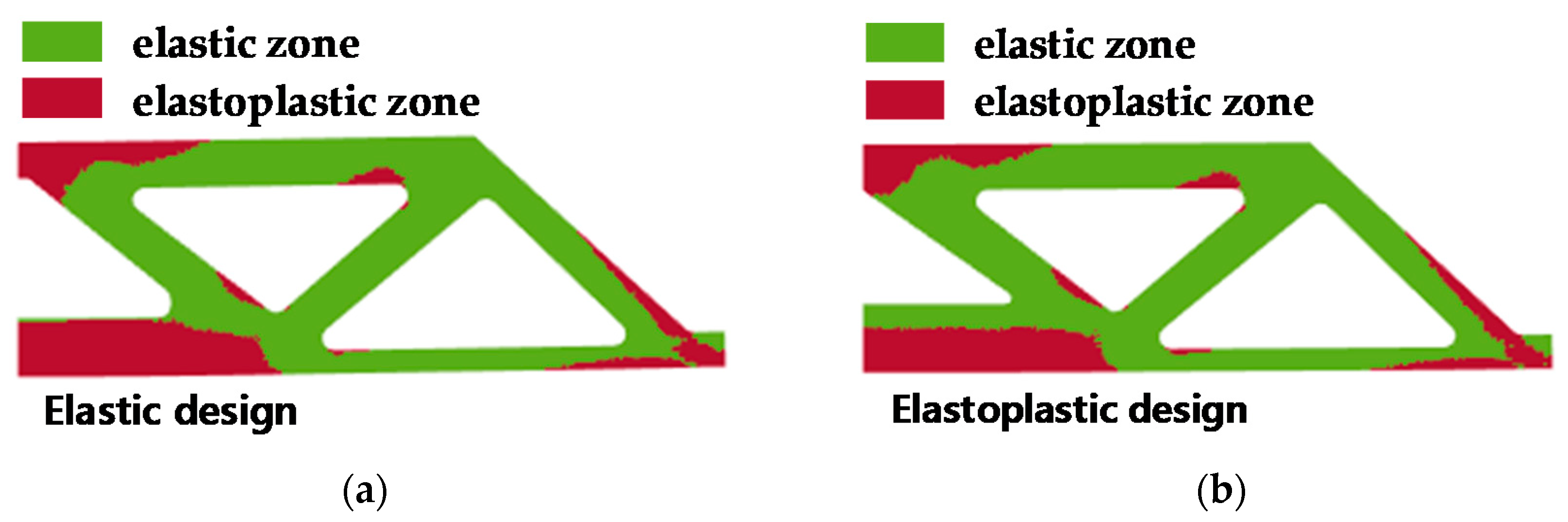
In the objective function, plastic work was separated from stain energy and the separated plastic work was selectively applied according to a deformation mode. In elastic deformation areas, strain energy was minimized, as in general cases. In elastoplastic deformation areas, only the plastic work was minimized for the purpose of suppressing plastic deformation. This method is able to focus on suppressing plastic deformation in the elastoplastic deformation areas while still accounting for elastic stiffness in the elastic deformation areas.
(3)
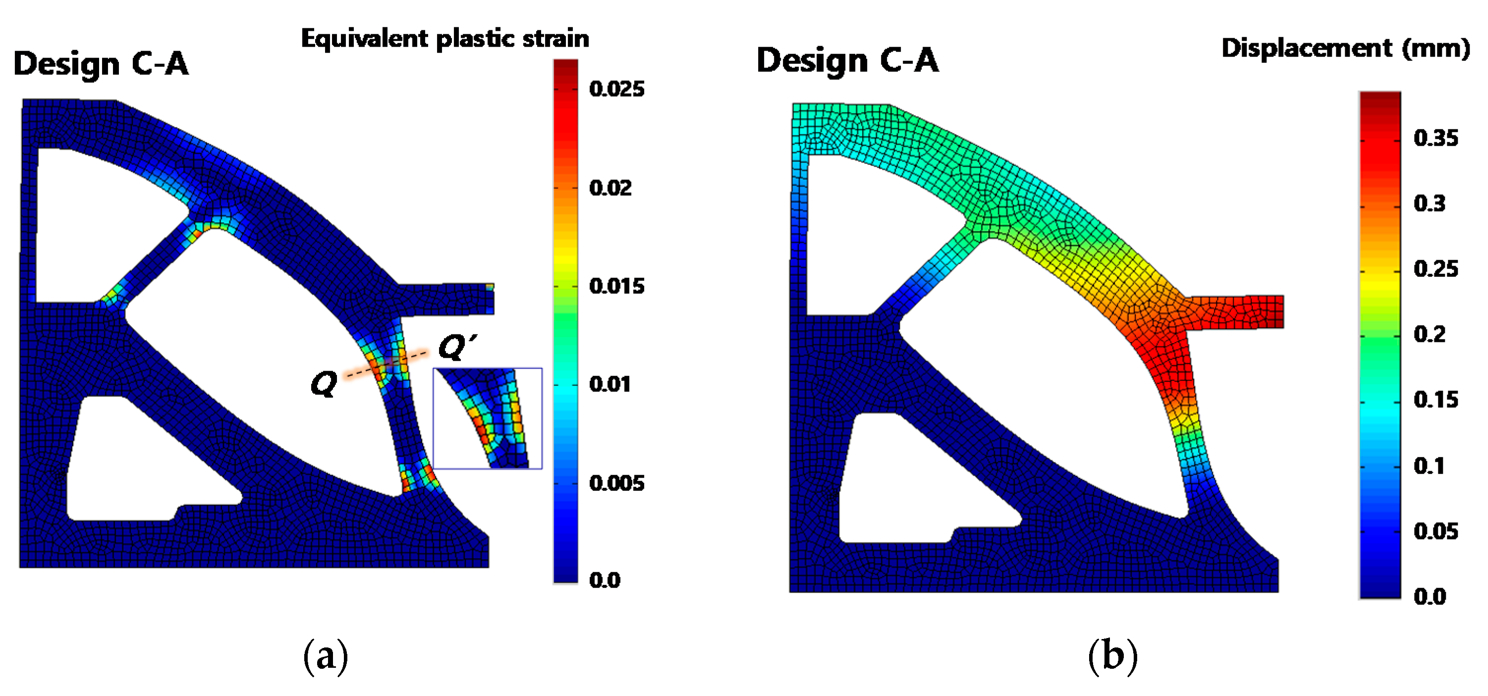
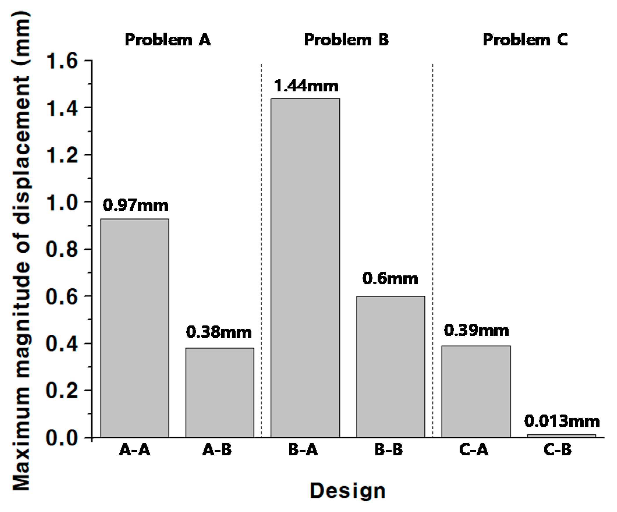
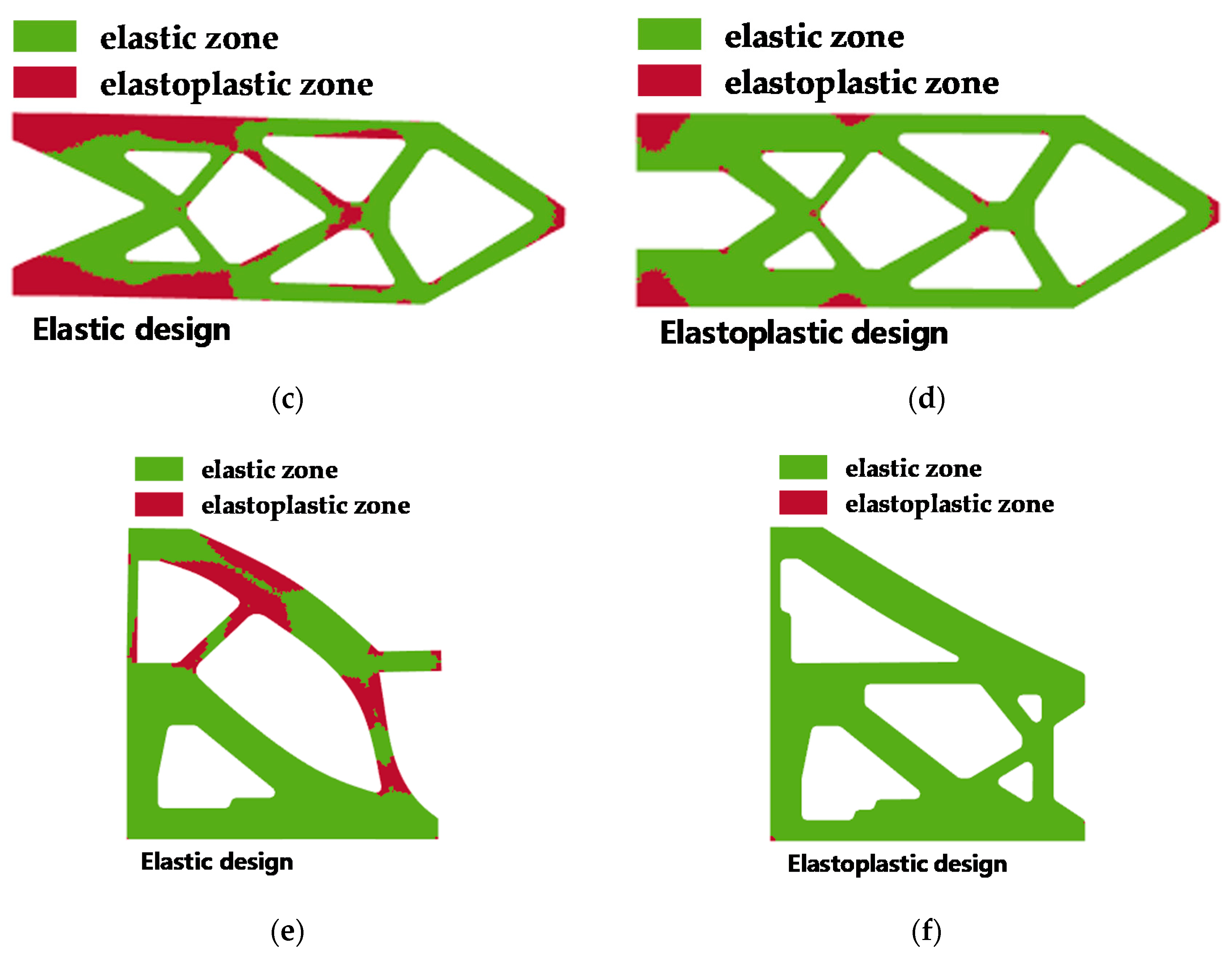
The structures designed while considering elastoplastic deformation strengthened the areas where plastic deformation occurs. The reinforced structures drastically reduced plastic strain and the magnitude of displacement when compared to shapes designed with only elastic deformation.
(4)
The structures designed with elastoplastic deformation can delay the beginning of plastic deformation and reduce plastically dissipated energy in the structures. This reduction and delay of the plastic deforming can decrease chances of plastic collapse.
(5)
The time step and loading condition affects the stability of the optimization. It is recommended to use appropriate time step and loading condition in optimization processes.
Based on the above results, this study shows that the selectively applied plastic work in the objective function can result in the design of safer supporting structures which reduce plastic deformation under conditions of large deformation.

Author Contributions

Conceptualization, E.-H.L.; methodology, E.-H.L.; software, E.-H.L.; validation, E.-H.L.; formal analysis, E.-H.L. and T.-H.K.; investigation, E.-H.L.; resources, T.-H.K.; data curation, T.-H.K.; writing—original draft preparation, E.-H.L. and T.-H.K.; writing—review and editing, E.-H.L. and T.-H.K.; visualization, T.-H.K.; supervision, E.-H.L.; project administration E.-H.L.; funding acquisition, E.-H.L. All authors have read and agreed to the published version of the manuscript.

Funding

This research was funded from the National Research Foundation of Korea (NRF) grant (No. 2020R1F1A1069535) funded by the Korea government.

Conflicts of Interest

The authors declare no conflict of interest.

References

  1. Wu, Y.; Li, Q.; Hu, Q.; Borgart, A. Size and Topology Optimization for Trusses with Discrete Design Variables by Improved Firefly Algorithm. Math. Probl. Eng. 2017, 2017, 1–12. [Google Scholar] [CrossRef] [Green Version]
  2. Liu, L.; Xing, J.; Yang, Q.; Luo, Y. Design of Large-Displacement Compliant Mechanisms by Topology Optimization Incorporating Modified Additive Hyperelasticity Technique. Math. Probl. Eng. 2017, 2017, 1–11. [Google Scholar] [CrossRef]
  3. Hatamizadeh, A.; Song, Y.; Hopkins, J.B. Optimizing the Geometry of Flexture System Topologies Using the Boundary Learning Optimization Tool. Math. Probl. Eng. 2018, 2018, 1–14. [Google Scholar] [CrossRef] [Green Version]
  4. Asadpoure, A.; Valdevit, L. Topology optimization of lightweight periodic lattices under simultaneous compressive and shear stiffness constraints. Int. J. Solids Struct. 2015, 60–61, 1–16. [Google Scholar] [CrossRef]
  5. Belhabib, S.; Guessasma, S. Compression performance of hollow structures: From topology optimization to design 3D printing. Int. J. Mech. Sci. 2017, 133, 728–739. [Google Scholar] [CrossRef]
  6. Bakhtiari-Shahri, M.; Moeenfard, H. Topology optimization of fundamental compliant mechanisms using a novel asymmetric beam flexture. Int. J. Mech. Sci. 2018, 135, 383–397. [Google Scholar] [CrossRef]
  7. Descamps, B.; Coelho, R.F. The nominal force method for truss geometry and topology optimization incorporating stability considerations. Int. J. Solids Struct. 2014, 51, 2390–2399. [Google Scholar] [CrossRef]
  8. Kook, J.; Jensen, J.S. Topology optimization of periodic microstructures for enhanced loss factor using acoustic-structure interaction. Int. J. Solids Struct. 2017, 122–123, 59–68. [Google Scholar] [CrossRef]
  9. Luo, Y.; Li, M.; Kang, Z. Topology optimization of hyperelastic structures with frictionless contact supports. Int. J. Solids Struct. 2016, 81, 373–382. [Google Scholar] [CrossRef]
  10. Tripathi, A.; Bajaj, A.K. Topology optimization and internal resonances in transverse vibrations of hyperelastic plates. Int. J. Solids Struct. 2016, 81, 311–328. [Google Scholar] [CrossRef]
  11. Penadés-Plà, V.; García-Segura, T.; Yepes, V. Robust Design Optimization for Low-Cost Concrete Box-Girder Bridge. Mathematics 2020, 8, 398. [Google Scholar] [CrossRef] [Green Version]
  12. Andreassen, E.; Clausen, A.; Schevenels, M.; Lazarov, B.S.; Sigmund, O. Efficient topology optimization in MATLAB using 88 lines of code. Struct. Multidiscip. Optim. 2011, 43, 1–16. [Google Scholar] [CrossRef] [Green Version]
  13. Andreassen, E.; Lazarov, B.S.; Sigmund, O. Design of manufacturable 3D extremal elastic microstructure. Mech. Mater. 2014, 69, 1–10. [Google Scholar] [CrossRef] [Green Version]
  14. Buhl, T.; Pedersen, C.B.W.; Sigmund, O. Stiffness design of geometrically nonlinear structures using topology optimization. Struct. Multidiscip. Optim. 2000, 19, 93–104. [Google Scholar] [CrossRef]
  15. Eschenauer, H.A.; Olhoff, N. Topology optimization of continuum structures: A review. Appl. Mech. Rev. 2001, 54, 331–390. [Google Scholar] [CrossRef]
  16. Petersson, J.; Sigmund, O. Slope constrained topology optimization. Int. J. Numer. Methods Eng. 1998, 41, 1417–1434. [Google Scholar] [CrossRef]
  17. Suzuki, K.; Kikuchi, N. A homogenization method for shape and topology optimization. Comput. Methods Appl. Mech. Eng. 1991, 93, 291–318. [Google Scholar] [CrossRef] [Green Version]
  18. Sigmund, O. A 99 line topology optimization code written in Matlab. Struct. Multidiscip. Optim. 2001, 21, 120–127. [Google Scholar] [CrossRef]
  19. Zhang, G.; Li, L.; Khandelwal, K. Topology optimization of structures with anisotropic plastic materials using enhanced assumed strain elements. Struct. Multidiscip. Optim. 2017, 55, 1965–1988. [Google Scholar] [CrossRef]
  20. Wallin, M.; Jönsson, V.; Wingren, E. Topology optimization based on finite strain plasticity. Struct. Multidiscip. Optim. 2016, 54, 783–793. [Google Scholar] [CrossRef]
  21. Schwarz, S.; Maute, K.; Ramm, E. Topology and shape optimization for elastoplastic structural response. Comput. Methods. Appl. Mech. Eng. 2001, 190, 2135–2155. [Google Scholar] [CrossRef]
  22. Blachowski, B.; Tauzowski, P.; Lógó, J. Yield limited optimal topology design of elastoplastic structures. Struct. Multidisc. Optim. 2020, 61, 1953–1976. [Google Scholar] [CrossRef]
  23. Herfelt, M.A.; Poulsen, P.N.; Hoang, L.C. Strength-based topology optimisation of plastic isotropic von Mises materials. Struct. Multidisc. Optim. 2019, 59, 893–906. [Google Scholar] [CrossRef] [Green Version]
  24. Alberdi, R.; Khandelwal, K. Topology optimization of pressure dependent elastoplastic energy absorbing structures with material damage constraints. Finite Elem. Anal. Des. 2017, 133, 42–61. [Google Scholar] [CrossRef]
  25. Huang, X.; Xie, Y.M.; Lu, G. Topology optimization of energy-absorbing structures. Int. J. Crashworthiness 2007, 12, 663–675. [Google Scholar] [CrossRef]
  26. Li, L.; Zhang, G.; Khandelwal, K. Topology optimization of energy absorbing structures with maximum damage constraint. Int. J. Numer. Methods Eng. 2017, 112, 737–775. [Google Scholar] [CrossRef]
  27. Li, L.; Zhang, G.; Khandelwal, K. Design of energy dissipating elastoplastic structures under cyclic loads using topology optimization. Struct. Multidiscip. Optim. 2017, 56, 391–412. [Google Scholar] [CrossRef]
  28. Barba, P.D.; Mognaschi, M.E.; Sieni, E. Many Objective Optimization of a Magnetic Micro-Electro-Mechanical (MEMS) Micromirror with Bounded MP-NSGA Algorithm. Mathematics 2020, 8, 1509. [Google Scholar] [CrossRef]
  29. Ziedan, H.A.; Rezk, H.; Al-Dhaifallah, M.; El-Zohri, E.H. Finite Element Solution of the Corona Discharge of Wire-Duct Electrostatic Precipitators at High Temperatures-Numerical Computation and Experimental Verification. Mathematics 2020, 8, 1406. [Google Scholar] [CrossRef]
  30. Bendsøe, M.P. Optimal shape design as a material distribution problem. Struct. Optim. 1989, 1, 193–202. [Google Scholar] [CrossRef]
  31. Mlejnek, H.P. Some aspects of the genesis of structures. Struct. Optim. 1992, 5, 64–69. [Google Scholar] [CrossRef]
  32. Bendsøe, M.P.; Sigmund, O. Material interpolation schemes in topology optimization. Arch. Appl. Mech. 1999, 69, 635–654. [Google Scholar] [CrossRef]
  33. Lee, E.H.; Yang, D.Y.; Yoon, J.W.; Yang, W.H. Numerical modeling and analysis for forming process of dual-phase 980 steel exposed to infrared local heating. Int. J. Solids Struct. 2015, 75–76, 211–224. [Google Scholar] [CrossRef]
  34. Yoon, J.W.; Yang, D.Y.; Chung, K. Elasto-plastic finite element method based on incremental deformation theory and continuum based shell elements for planar anisotropic sheet materials. Comput. Methods. Appl. Mech. Eng. 1999, 174, 23–56. [Google Scholar] [CrossRef]
  35. Hockett, J.E.; Sherby, O.D. Large strain deformation of polycrystalline metals at low homologous temperatures. J. Mech. Phys. Solids. 1975, 23, 87–98. [Google Scholar] [CrossRef]
  36. Lee, E.H.; Stoughton, T.B.; Yoon, J.W. A new strategy to describe nonlinear elastic and asymmetric plastic behaviors with one yield surface. Int. J. Plast. 2017, 98, 217–238. [Google Scholar] [CrossRef]
  37. Lee, E.H.; Choi, H.; Stoughton, T.B.; Yoon, J.W. Combined anisotropic and distortion hardening to describe directional response with Bauschinger effect. Int. J. Plast. 2019, 122, 73–88. [Google Scholar] [CrossRef]
  38. Lee, E.H.; Rubin, M.B. Modeling anisotropic inelastic effects in sheet metal forming using microstructual vectors–Part I: Theory. Int. J. Plast. 2020, 134, 102783. [Google Scholar] [CrossRef]
  39. Bendsøe, M.P. Optimization of Structural Topology: Shape and Material; Springer: Berlin/Heidelberg, Germany; New York, NY, USA, 1995. [Google Scholar]
  40. Bruns, T.E.; Tortorelli, D.A. Topology optimization of non-linear elastic structures and compliant mechanisms. Comput. Methods. Appl. Mech. Eng. 2001, 190, 3443–3459. [Google Scholar] [CrossRef]
Figure 1. Stress-strain curve of the material.
Mathematics 08 02062 g001
Figure 2. Flow chart of the numerical algorithm.
Mathematics 08 02062 g002
Figure 3. Design examples: (a) Messerschmitt–Bölkow–Blohm (MBB) beam problem (problem A); (b) Tip loaded cantilever beam problem (problem B); (c) Structure with a spring supporter (problem C).
Mathematics 08 02062 g003aMathematics 08 02062 g003b
Figure 4. Optimized shape for the MBB beam: (a) Under the elastic deformation assumption (design A–A); (b) Elastoplastic deformation (design A–B).
Mathematics 08 02062 g004
Figure 5. Optimized shape for the cantilever beam: (a) Under the elastic deformation assumption (design B–A); (b) Elastoplastic deformation (design B–B).
Mathematics 08 02062 g005aMathematics 08 02062 g005b
Figure 6. Optimized shape for the structure with a spring: (a) Under the elastic deformation assumption (design C–A); (b) Elastoplastic deformation (design C–B).
Mathematics 08 02062 g006
Figure 7. FEM models: (a) Design A–A; (b) Design A–B; (c) Design B–A; (d) Design B–B; (e) Design C–A; (f) Design C–B.
Mathematics 08 02062 g007
Figure 8. Simulation results of problem A: (a) Plastic strain of design A–A; (b) Displacement of design A–A; (c) Plastic strain of design A–B; (d) Displacement of design A–B.
Mathematics 08 02062 g008aMathematics 08 02062 g008b
Figure 9. Simulation results of problem B: (a) Plastic strain of design B–A; (b) Displacement of design B–A; (c) Plastic strain of design B–B; (d) Displacement of design B–B.
Mathematics 08 02062 g009
Figure 10. Simulation results of problem C: (a) Plastic strain of design C–A; (b) Displacement of design C–A; (c) Plastic strain of design C–B; (d) Displacement of design C–B.
Mathematics 08 02062 g010aMathematics 08 02062 g010b
Figure 11. Maximum magnitude of displacement in each design.
Mathematics 08 02062 g011
Figure 12. Contour of the elastoplastic zone: (a) Design A–A; (b) Design A–B; (c) Design B–A; (d) Design B–B; (e) Design C–A; (f) Design C–B.
Mathematics 08 02062 g012aMathematics 08 02062 g012b
Figure 13. Plastic strain distribution according to a section; (a) Plastic strain of the section O-O’; (b) Plastic strain of the section P-P’; (c) Plastic strain of the section Q-Q’.
Mathematics 08 02062 g013
Figure 14. Plastic work according to time; (a) Plastic work of designs A–A and A–B; (b) Plastic work of designs B–A and B–B; (c) Plastic work of designs C–A and C–B.
Mathematics 08 02062 g014aMathematics 08 02062 g014b
Figure 15. FEM simulation with respect to the difference loading conditions: (a) f = fcollapse; (b) f = 0.9fcollapse; (c) f = 0.83fcollapse; (d) f = 0.55fcollapse.
Mathematics 08 02062 g015
Figure 16. Time increment and loading condition effect.
Mathematics 08 02062 g016
Table 1. Material parameters of the modified Hockett–Sherby model.
Parameters of the Modified Hockett–Sherby Model
A (MPa)B (MPa)CbD (MPa)
568.74368.191.810.6078.1
Publisher’s Note: MDPI stays neutral with regard to jurisdictional claims in published maps and institutional affiliations.

