Article

The Geometry of a Randers Rotational Surface with an Arbitrary Direction Wind

by
Rattanasak Hama
1,*,† and
Sorin V. Sabau
2,†
1
Faculty of Science and Industrial Technology, Surat Thani Campus, Prince of Songkla University, Surat Thani 84000, Thailand
2
Department of Biological Sciences, Sapporo Campus, Tokai University, Sapporo 005-8601, Japan
*
Author to whom correspondence should be addressed.
These authors contributed equally to this work.
Mathematics 2020, 8(11), 2047; https://doi.org/10.3390/math8112047
Submission received: 5 October 2020 / Revised: 5 November 2020 / Accepted: 11 November 2020 / Published: 17 November 2020
(This article belongs to the Special Issue Complex and Contact Manifolds)

Abstract

:
In the present paper, we study the global behaviour of geodesics of a Randers metric, defined on Finsler surfaces of revolution, obtained as the solution of the Zermelo’s navigation problem. Our wind is not necessarily a Killing field. We apply our findings to the case of the topological cylinder R × S 1 and describe in detail the geodesics behaviour, the conjugate and cut loci.

1. Introduction

A Finsler surface ( M , F ) is a geometrical structure defined on a smooth 3-manifold Σ T M whose the canonical projection π : Σ M is a surjective submersion such that for each x M , the π -fiber Σ x = π 1 ( x ) is a strictly convex curve including the origin O x T x M . Here, we denote by T M the tangent bundle of M. This is actually equivalent to saying that ( M , F ) is a surface M endowed with a Minkowski norm in each tangent space T x M that varies smoothly with the base point x M all over the manifold. Obviously, Σ is the unit sphere bundle { ( x , y ) T M : F ( x , y ) = 1 } , also called the indicatrix bundle. Even though the these notions are defined for arbitrary dimension, we restrict to surfaces hereafter [1].
On the other hand, such a Finsler structure ( M , F ) defines a 2-parameter family of oriented curves, or paths, on the surface M, one going in each oriented direction passing through every point. This is a special case of so-called Path Geometry. We recall that, roughly speaking, a path geometry on a surface M is a family of curves on M such that through each point x M there exists a unique curve in the family going in each tangent direction at x (the simplest case is a family of lines in the Euclidean plane).
To be more precise, a path geometry on a surface M is given by a foliation P defined on the projective tangent bundle P T M by contact curves that are transverse to the fibers of the canonical projection π : P T M M . Observe that even though P T M is independent of any norm F, actually there is a Riemannian isometry between P T M and Σ , a fact that allows us to identify them in the Finslerian case [2].
The 3-manifold P T M is naturally endowed with a contact structure. Indeed, for a curve to be a smooth, immersed curve γ : ( a , b ) M , we denote γ ^ : ( a , b ) P T M its canonical lift to the projective tangent bundle P T M . Since the canonical projection is a submersion, it results that, for each line L P T M , the linear map π * , L : T L P T M T x M , is surjective, here π ( L ) = x M . Hence, E L : = π * , L 1 ( L ) T L P T M is a 2-plane in T L P T M that defines a contact distribution and thus a contact structure on P T M . The curve on P T M is called a contact curve if it is tangent to the contact distribution E. Clearly, the canonical lift γ ^ to P T M of the curve γ on M is by definition a contact curve.
If ( M , F ) is a Finsler surface, then the 3-manifold Σ is endowed with a canonical coframe ( ω 1 , ω 2 , ω 3 ) satisfying the structure equations
d ω 1 = I ω 1 ω 3 + ω 2 ω 3 d ω 2 = ω 3 ω 1 d ω 3 = K ω 1 ω 2 J ω 1 ω 3 ,
where the functions I , J and K : T M R are the Cartan scalar, the Landsberg curvature and the Gauss curvature, respectively (see [1] or [3] for details). The 2-plane field D : = e ^ 2 , e ^ 3 defines a contact structure on Σ , where we denote ( e ^ 1 , e ^ 2 , e ^ 3 ) the dual frame of ( ω 1 , ω 2 , ω 3 ) . Indeed, it can be seen that the 1-form η : = A ω 1 is a contact form for any function A 0 on Σ . The structure Equation (1) imply η d η = A 2 ω 1 ω 2 ω 3 0 . Observe that in the Finslerian case, we actually have two foliations on the 3-manifold Σ :
  • P = { ω 1 = 0 , ω 3 = 0 } the geodesic foliation on Σ , that is the leaves are curves in Σ tangent to the geodesic spray e ^ 2 ;
  • Q = { ω 1 = 0 , ω 2 = 0 } the indicatrix foliation of Σ , that is the leaves are indicatrix curves in Σ tangent e ^ 3 .
The pair ( P , Q ) is called sometimes a generalized path geometry (see [3]).
The (forward) integral length of a regular piecewise C -curve γ : [ a , b ] M on a Finsler surface ( M , F ) is given by
L γ : = i = 1 k t i 1 t i F ( γ ( t ) , γ ˙ ( t ) ) d t ,
where γ ˙ = d γ d t is the tangent vector along the curve γ | [ t i 1 , t i ] .
A regular piecewise C -curve γ on a Finsler manifold is called a (forward) geodesic if ( L γ ) ( 0 ) = 0 for all piecewise C -variations of γ keeping its ends fixed (this can be characterized by using the Chern connection or other Finsler connection [1]). Observe that the canonical lift of a geodesic γ to P T M gives the geodesics foliation P described above.
The integral length of a curve allows to define the Finslerian distance between points on M. For two points p , q M , let Ω p , q be the set of all regular piecewise C -curves γ : [ a , b ] M , γ ( a ) = p and γ ( b ) = q . Then the function
d : M × M [ 0 , ) , d ( p , q ) : = inf γ Ω p , q L γ
is called the Finslerian distance on M. Observe that d is not symmetric in general.
A Finsler manifold ( M , F ) is called forward geodesically complete if any geodesic γ : [ a , b ) M can be extended to a geodesic γ : [ a , ) M . The equivalence between forward completeness as metric space and geodesically completeness is given by the Hopf–Rinow Theorem Finsler case (see, e.g., [1], p. 168). Same is true for backward geodesics.
Any geodesic γ starting from a point p in a compact Finsler manifold loses its global minimality at a point q on γ . This point q is called a cut point of p along γ . One can define the cut locus of a point p as the set of all cut points along all geodesics starting from the point p. This kind of point often appears as an obstruction in global theorems in differential geometry, it also appears in analysis as a singular points set. Observe that the cut locus of a point p is actually the closure of the set of non-differentiable points of the distance function from the point p. The structure of the cut locus is important in optimal control problems and quantum dynamics.
The cut locus was discovered by H. Poincaré in 1905. For a 2-dimensional analytical sphere, S. B. Myers has shown that the cut locus of a point is a finite tree for Riemannian and Finsler metrics [4]. For an analytic Riemannian manifold, M. Buchner has proved that the cut locus of a point p is triangulable, and has obtained its local structure [5,6]. It is known that the cut locus may have a quite complex structure. Indeed, H. Gluck and D. Singer have constructed a C Riemannian manifold having a point with non-triangulable cut locus (see [7] or [8] for an exposition). It was also shown that there exist C k -Riemannian and Finsler structures on spheres with a special point whose cut locus is a fractal [9].
In the present paper, we will study the local and global behaviour of the geodesics of a Finsler metric of revolution on topological cylinders. In special, we will determine the structure of the cut locus on the cylinder for such metrics and compare it with the Riemannian case.
We will focus on Finsler metrics of Randers type obtained as solutions of the Zermelo’s navigation problem, for the navigation data ( M , h ) , where h is the canonical Riemannian metric on the topological cylinder h = d r 2 + m 2 ( r ) d θ 2 , and W = A ( r ) r + B θ is a vector field on M. Observe that our wind is more general than a Killing vector field, hence our theory presented here is a generalization of the classical study of geodesics and cut locus for Randers metrics obtained as solutions of the Zermelo’s navigation problem with Killing vector fields studied in [10,11] (see also [12] for another attempt to generalize the Zermelo’s navigation problem). Nevertheless, by taking the wind W in this way, we obtain a quite general Randers metric on M which is a Finsler metric of revolution and whose geodesics and cut locus can be computed explicitly.
Our paper is organized as follows. In Section 2, we recall basics of Finsler geometry using the Randers metrics that we will actually use in order to obtain explicit information on the geodesics behaviour and cut locus structure. We introduce an extension of the Zermelo’s navigation problem for Killing winds to a more general case W ˜ = V + W , where only W is Killing. In Section 3, we show that the geodesics, conjugate locus and cut locus can be determined in this case as well. In Section 3.1 and Section 3.2, we address the cases when β is closed one-form and W is F-Killing field, respectively.
In Section 4, we describe the theory of general Finsler surfaces of revolution. In the case this, Finsler metric is a Riemannian one, we obtain the theory of geodesics and cut locus known already [13,14].
In Section 4.3, we consider the general wind W = A ( r ) r + B θ which obviously is not Killing with respect to h, where A = A ( r ) is a bounded function and B is a constant and determine its geometry here. Essentially, we are reducing the geodesics theory of the Finsler metric F ˜ , obtained from the Zermelo’s navigation problem for ( M , h ) and W ˜ , to the theory of a Riemannian metric ( M , α ) .
Moreover, in the particular case W ˜ = A r + B θ in Section 4.4, where A , B are constants, the geodesic theory of F ˜ can be directly obtained from the geometry of the Riemannian metric ( M , h ) . A similar study can be done for the case W = A ( r ) r . We leave a detailed study of these Randers metrics to a forthcoming research.

2. Finsler Metrics. The Randers Case

Finsler structures are one of the most natural generalization of Riemannian metrics. Let us recall here that a Finsler structure on a real smooth n-dimensional manifold M is a function F : T M [ 0 , ) which is smooth on T M ˜ = T M \ O , where O is the zero section, with the homogeneity property F ( x , λ y ) = λ F ( x , y ) , for all λ > 0 and all y T x M . It is also requested that the Hessian matrix is strongly convex, i.e., the matrix
g i j : = 1 2 2 F 2 y i y j ( x , y )
is positive definite at any point ( x , y ) T M .

2.1. An Ubiquitous Family of Finsler Structures: The Randers Metrics

Originally introduced in general relativity, Randers metrics are the most natural family of Finsler structures [1].
A Randers metric on a surface M is obtained by a rigid translation of an ellipse in each tangent plane T x M such that the origin of T x M remains inside it.
Formally, on a Riemannian manifold ( M , α ) , a Randers metric is a Finsler structure ( M , F ) whose fundamental function F : T M [ 0 , ) can be written as
F ( x , y ) = α ( x , y ) + β ( x , y ) ,
where α ( x , y ) = a i j ( x ) y i y j and β ( x , y ) = b i ( x ) y i , such that the Riemannian norm of β is less than 1, i.e., b 2 : = a i j b i b j < 1 .
It is known that Randers metrics are solutions of the Zermelo’s navigation problem [15] which we recall here.
Consider a ship sailing on the open sea in calm waters. If a mild breeze comes up, how should the ship be steered in order to reach a given destination in the shortest time possible?
The solution was given by Zermelo in the case the open sea is an Euclidean space, by [16] in the Riemannian case and studied in detailed in [17].
Indeed, for a time-independent wind W T M , on a Riemannian manifold ( M , h ) , the minimizing travel-time paths coincide with the geodesics of the Randers metric
F ( x , y ) = α ( x , y ) + β ( x , y ) = λ y h 2 + W 0 λ W 0 λ ,
where W = W i ( x ) x i , y h 2 = h ( y , y ) , λ = 1 W h 2 , and W 0 = h ( W , y ) . Requiring W h < 1 , we obtain a positive definite Finslerian norm. In components, a i j = 1 λ h i j + W i λ W j λ , b i ( x ) = W i λ , where W i = h i j W j (see [18] for a general discussion).
The Randers metric obtained above is called the solution of the Zermelo’s navigation problem for the navigation data ( M , h ) and W.
Remark 1.
Obviously, at any x M , the condition F ( y ) = 1 is equivalent to y W h = 1 fact that assures that, indeed, the indicatrix of ( M , F ) in T x M is obtained from the unit sphere of h by translating it along W ( x ) (see Figure 1).
More generally, the Zermelo’s navigation problem can be considered where the open sea is a given Finsler manifold (see [16]).
We have
Proposition 1.
Let ( M , F ) be a Finsler manifold and W a vector field on M such that F ( W ) < 1 . Then the solution of the Zermelo’s navigation problem with navigation data F , W is the Finsler metric F ˜ obtained by solving the equation
F ( y F ˜ W ) = F ˜ , f o r a n y y T M .
Indeed, if we consider the Zermelo’s navigation problem where the open sea is the Finsler manifold ( M , F ) and the wind W, by rigid translation of the indicatrix Σ F , we obtain the closed, smooth, strongly convex indicatrix Σ F ˜ , where F ˜ is solution of the equation F y F ˜ W = 1 which is clearly equivalent to (3) due to positively of F ˜ and homogeneity of F.
To get a genuine Finsler metric F ˜ , We need for the origin O x T x M to belong to the interior of Σ F ˜ = Σ F + W , that is F ( W ) < 1 .
Remark 2.
Consider the Zermelo’s navigation problem for ( M , F ) and wind W, where F is a (positive-defined) Finsler metric. If we solve the equation
F y F ˜ W = 1 F ( y F ˜ W ) = F ˜
we obtain the solution of this Zermelo’s navigation problem.
In order that F ˜ is Finsler, we need to check:
 (i)
F ˜ is strongly convex, and
 (ii)
the indicatrix of F ˜ includes the origin O x T x M .
Since indicatrix of F ˜ is the rigid translation by W of the indicatrix of F, and this is strongly convex, it follows indicatrix of F ˜ is also strongly convex.
Hence, we only need to check (ii).
Denote
B F ( 1 ) : = { y T x M : F ( y ) < 1 } , B ˜ F ˜ ( 1 ) : = { y T x M : F ˜ ( y ) < 1 }
the unit balls of F and F ˜ , respectively.
The Zermelo’s navigation problem shows
B F ˜ ( 1 ) = B F ( 1 ) + W .
Thus,
O x B F ˜ ( 1 ) O x B F ( 1 ) + W W B F ( 1 ) F ( W ) < 1 .
Hence, indicatrix of F ˜ include O x , i.e., F ( W ) < 1 .
Proposition 2.
Let ( M , F = α + β ) be a Randers space and W = W i ( x ) x i a vector field on M. Then, the solution of the Zermelo’s navigation problem, with navigation data ( M , F ) and W, is also a Randers metric F ˜ = α ˜ + β ˜ , where
a ˜ i j = 1 η a i j b i b j + W i b i [ 1 + β ( W ) ] η W j b j [ 1 + β ( W ) ] η , b ˜ i = W i b i [ 1 + β ( W ) ] η ,
and η = [ 1 + β ( W ) ] 2 α 2 ( W ) , W i = a i j W j .
Proof of Proposition 2.
Let us consider the equation
F y F ˜ W = 1
which is equivalent to
F ( y F ˜ W ) = F ˜
due to positively of F ˜ and 1-positive homogeneity of F.
If we use F = α + β , it follows
α ( y F ˜ W ) = F ˜ β ( y F ˜ W ) ,
hence, by using the linearity of β , i.e., β ( y F ˜ W ) = β ( y ) F ˜ β ( W ) , where β ( y ) = b i y i , β ( W ) = b i W i , and squaring this formula, we get the equation
α 2 ( y F ˜ W ) = [ F ˜ ( 1 + β ( W ) ) β ( y ) ] 2 .
Observe that
α 2 ( y F ˜ W ) = α 2 ( y ) 2 F ˜ y , W α + F ˜ 2 α 2 ( W ) ,
and
[ F ˜ β ( y F ˜ W ) ] 2 = [ 1 + β ( W ) ] 2 F ˜ 2 2 F ˜ β ( y ) [ 1 + β ( W ) ] + β 2 ( y ) ,
substituting (6), (7) in (5) gives the quadratic equation
η F ˜ 2 + 2 F ˜ y , W B [ 1 + β ( W ) ] α [ α 2 ( y ) β 2 ( y ) ] = 0 ,
where · , · α is the scalar product with respect to the Riemannian metric α , B : = b i x i = ( a i j b j ) x i and η : = [ 1 + β ( W ) ] 2 α 2 ( W ) , i.e.,
y , W B [ 1 + β ( W ) ] α = a i j y i ( W j b j [ 1 + β ( W ) ] ) = y , W α β ( y ) [ 1 + β ( W ) ] .
The discriminant of (8) is
D = { y , W α β ( y ) [ 1 + β ( W ) ] } 2 + η [ α 2 ( y ) β 2 ( y ) ] .
Let us observe that F ( W ) < 1 implies η > 0 . Indeed,
F ( W ) = α ( W ) β ( W ) < 1 α 2 ( W ) < [ 1 + β ( W ) ] 2
hence, η > 0 .
Moreover, observe that
D = { η ( a i j b i b j ) + ( W i b i [ 1 + β ( W ) ] ) ( W j b j [ 1 + β ( W ) ] ) } y i y j .
The solution of the quadratic Equation (8) is given by
F ˜ = y , W B [ 1 + β ( W ) ] α 2 + η [ α 2 ( y ) β 2 ( y ) ] η < y , W B [ 1 + β ( W ) ] > α η ,
or, equivalently
F ˜ = { η ( a i j b i b j ) + ( W i b i [ 1 + β ( W ) ] ) ( W j b j [ 1 + β ( W ) ] ) } y i y j η { W i b i [ 1 + β ( W ) ] } y i η ,
that is, F ˜ = α ˜ + β ˜ , where a ˜ i j and b ˜ i are given by (4).
Observe that a ˜ i j is positive defined. Indeed, for any v T M , α ˜ 2 ( v , v ) = a ˜ i j v i v j = η [ α 2 ( v ) β 2 ( v ) ] + v , W B [ 1 + β ( W ) ] α 2 .
On the other hand, since F = α + β is Randers metric, F ( X ) > 0 for any tangent vector X T M , thus for X = v and X = v we get α ( v ) + β ( v ) > 0 and α ( v ) β ( v ) > 0 , respectively; hence, α 2 ( v ) β 2 ( v ) > 0 for any v T M .
This implies a ˜ i j is positive defined. □

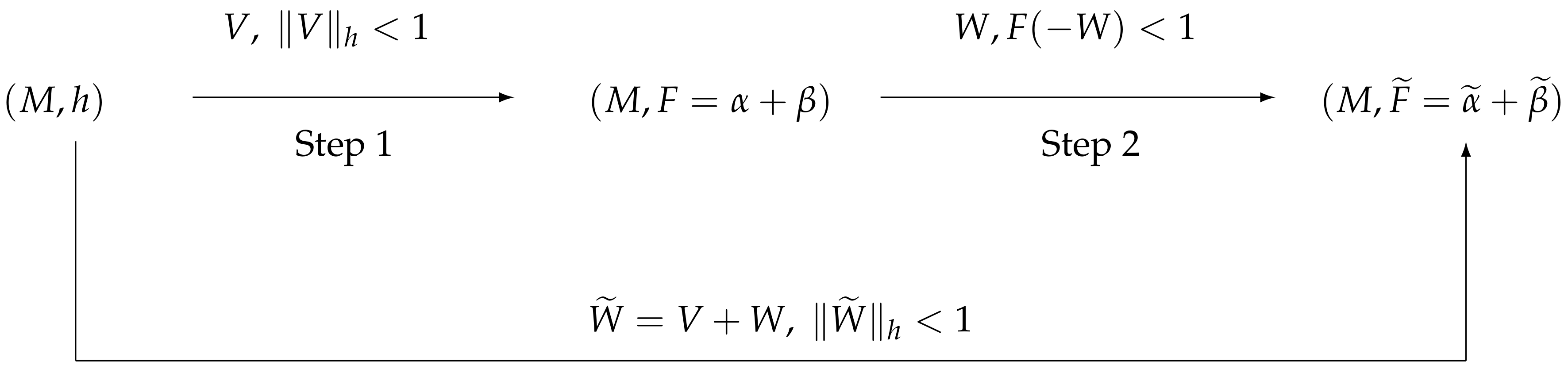
2.2. A Two Steps Zermelo’s Navigation

We have discussed in the previous section the Zermelo’s navigation when the open sea is a Riemannian manifold and when it is a Finsler manifold, respectively.
In order to obtain a more general version of the navigation, we combine these two approaches as in the following diagram (see Figure 2).
Mathematically, we have
Theorem 1.
Let ( M , h ) be a Riemannian manifold and V, W two vector fields on M.
Let us consider the Zermelo’s navigation problems on M with the following data
 (I)
Riemannian metric ( M , h ) with wind V + W and assume condition V + W h < 1 ;
 (II)
Finsler metric ( M , F ) with wind W and assume W satisfies condition F ( W ) < 1 , where F = α + β is the solution of the Zermelo’ s navigation problem for the navigation data ( M , h ) with wind V, such that V h < 1 ,
respectively.
Then, the above Zermelo’s navigation problems (I) and (II) have the same solution F ˜ = α ˜ + β ˜ .
Proof of Theorem 1.
Let us consider case (I), i.e., the sea is the Riemannian metric ( M , h ) with the wind W ˜ : = V + W such that V + W h < 1 . The associated Randers metric through the Zermelo’s navigation problem is given by α ˜ + β ˜ , where
a ˜ i j : = 1 Λ h i j + W ˜ i Λ W ˜ j Λ , b ˜ i : = W ˜ i Λ ,
and Λ = 1 W ˜ h 2 = 1 V + W h 2 , W ˜ i = h i j W ˜ j .
Observe that (9) are actually equivalent to
a ˜ i j : = 1 Λ h i j + V i ( h ) + W i ( h ) Λ V j ( h ) + W j ( j ) Λ , b ˜ i : = W i ( h ) Λ V i ( h ) Λ ,
where V i ( h ) = h i j V j and W i ( h ) = h i j W j .
Next, we will consider the case (II) which we regard as a two steps Zermelo type navigation:
Step 1. Consider the Zermelo’s navigation with data ( M , h ) and wind V, V h 2 < 1 with the solution F = α + β , where
a i j = 1 λ h i j + V i ( h ) λ V j ( h ) λ , b i = V i ( h ) λ ,
and λ = 1 V h 2 , V i ( h ) = h i j V j .
Step 2. Consider the Zermelo’s navigation with data ( M , F = α + β ) obtained at step 1, and wind W such that F ( W ) < 1 , with solution F ˜ = α ^ + β ^ (see Proposition 2), where
a ^ i j = 1 η ( a i j b i b j ) + W i ( α ) b i [ 1 + β ( W ) ] η W j ( α ) b j [ 1 + β ( W ) ] η , b ^ i = W i ( α ) η
with
η = [ 1 + β ( W ) ] 2 α 2 ( W ) , and W i ( α ) = a i j W j .
We will show that a ˜ i j = a ^ i j and b ˜ i = b ^ i , respectively, for all indices i , j { 1 , , n } . It is trivial to see that Λ = λ W h 2 2 V , W h , where · , · h is the scalar product with respect to the Riemannian metric h.
Next, by straightforward computation we get
α 2 ( W ) = a i j W i W j = 1 λ W h 2 + h ( V , W ) λ 2 , β ( W ) = h ( V , W ) λ .
It follows that
η = 1 h ( V , W ) λ 2 1 λ W h 2 h 2 ( V , W ) λ 2 = 1 2 h ( V , W ) λ 1 λ W h 2 ,
hence, we get
η = Λ λ .
In a similar manner,
W i ( α ) b i [ 1 + β ( W ) ] η = 1 η h i j W j λ + V i ( h ) λ V j ( h ) W j λ + V i ( h ) λ 1 h ( V , W ) λ ,
hence, we obtain
W i ( α ) b i ( 1 + β ( W ) ) η = W i ( h ) + V i ( h ) Λ ,
that is b ˜ i = b ^ i .
It can be also seen that
1 η ( a i j b i b j ) = 1 Λ h i j ,
hence, a ˜ i j = a ^ i j and the identity of formulas (9) and (11) is proved. In order to finish the proof we show that the conditions
(i) V + W h 2 < 1 and (ii) V h 2 < 1 and F ( W ) < 1 are actually equivalent.
Geometrically speaking, the 2-steps Zermelo’s navigation is the rigid translation of Σ h by V followed by the rigid translation of Σ F by W. This is obviously equivalent to the rigid translation of Σ h by W ˜ = V + W .
The geometrical meaning of (i) is that the origin O x T x M is in the interior of the translated indicatrix Σ F ˜ (see Figure 3). On the other hand, the relation in (ii) shows that the origin O x is in the interior of the translated indicatrix Σ h by V and Σ F 1 by W.
This equivalence can also be checked analytically.
For initial data ( M , h ) and V, we obtain by Zermelo’s navigation the Randers metric F = α + β , where
a i j = 1 λ h i j + V i λ V j λ , b i = V i λ ,
with V i = h i j V j and λ = 1 V h 2 < 1 .
Consider another vector field W and compute
F ( W ) = 1 λ W h 2 + V i W i λ 2 + V i W i λ = 1 λ λ W h 2 + h 2 ( V , W ) + h ( V , W ) .
Let us assume F ( W ) < 1 , hence
λ W h 2 + h 2 ( V , W ) + h ( V , W ) < λ ,
i.e.,
λ W h 2 + h 2 ( V , W ) < [ λ h ( V , W ) ] 2 W h 2 < λ 2 h ( V , W ) W + V h 2 < 1 .
Conversely, if V + W h 2 < 1 , by reversing the computation above, we obtain F ( W ) < 1 , provided λ h ( V , W ) > 0 .
Indeed, observe that V + W h 2 < 1 actually implies λ h ( V , W ) > 0 , because 1 V h 2 h ( V , W ) = 1 h ( V , V + W ) > 0 h ( V , V + W ) < 1 .
However, using V h < 1 and V + W h < 1 , the Cauchy–Schwartz inequality gives h ( V , V + W ) V h V + W h < 1 . □
Remark 3.
The 2-steps Zermelo’s navigation problem discussed above, can be generalized to k-steps Zermelo’s navigation.
Let ( M , F ) be a Finsler space and let W 0 , W 1 , , W k 1 be k linearly independent vector fields on M. We consider the following k-step Zermelo’s navigation problem.
Step 0. F 1 solution of ( M , F 0 , W 0 ) with F 0 ( W 0 ) < 1 , i.e.,
   solution of F 0 y F 1 W 0 = 1 .
Step 1. F 2 solution of ( M , F 1 , W 1 ) with F 1 ( W 1 ) < 1 , i.e.,
   solution of F 1 y F 2 W 1 = 1 .
Step k 1 . F k solution of ( M , F k 1 , W k 1 ) with F k 1 ( W k 1 ) < 1 , i.e.,
   solution of F k 1 y F k W k 1 = 1 .
Then, F k is the Finsler metric obtained as solution of the Zermelo’s navigation problem with data F 0 , W ˜ : = W 0 + + W k 1 with condition F 0 ( W ˜ ) < 1 .

3. Geodesics, the Conjugate and Cut Loci

We will study the relation between the geodesics behaviour of the Riemannian metrics h, α , F and F ˜ in Figure 2.

3.1. The Case β Closed

We start with the case when β obtained in Step 1 is closed.
Proposition 3.
Let ( M , h ) be a Riemannian manifold, V a vector field such that V h < 1 , and let F = α + β be the solution of the Zermelo’s navigation with data ( M , h ) and V.
Then, d β = 0 if and only if V satisfies the differential equation
d η = d log λ η ,
where η = V i ( x ) d x i , V i = h i j V j , and λ = 1 V h 2 .
Proof of Proposition 3.
Observe that b i = V i λ is equivalent to λ β = η , hence d λ β + λ d β = d η and using d β = 0 we obtain
d λ β = d η .
By using β = 1 λ η , we get (13). The converse is easy to show taking into account that λ 0 . □
Remark 4.
The Equation (13) can be written in coordinates
V i x j V j x i d x i d x j = log λ x i d x i ( V j d x j ) ,
that is,
V i x j V j x i = log λ x i V j log λ x j V i .
In the 2-dimensional case, we get the 1st order PDE
V 1 x 2 V 2 x 1 = 1 λ h i j x 1 V 2 h i j x 2 V 1 V i V j 2 λ V i V i x 1 V 2 V i x 2 V 1 , i , j = 1 , 2 .
It can easily be seen that in the case of a surface of revolution h = d r 2 + m 2 ( r ) d θ 2 the wind V = A ( r ) r is a solution of (13) and of (14).
Theorem 2.
Let ( M , h ) be a simply connected Riemannian manifold and V = V i x i a vector field on M such that V h < 1 , and let F = α + β be the Randers metric obtained as the solution of the Zermelo’s navigation problem with this data.
If V satisfies the differential relation
d η = d ( log λ ) η ,
where η = V i ( x ) d x i , V i = h i j V j , then the followings hold good.
 (i)
There exists a smooth function f : M R such that β = d f .
 (ii)
The Randers metric F is projectively equivalent to α, i.e., the geodesics of ( M , F ) coincide with the geodesics of the Riemannian metric α as non-parameterized curve.
 (iii)
The Finslerian length of any C piecewise curve γ : [ a , b ] M on M joining the points p and q is given by
L F ( γ ) = L α ( γ ) + f ( q ) f ( p ) ,
where L α ( γ ) is the Riemannian length with respect to α of γ.
 (iv)
The geodesic γ is minimizing with respect to α if and only if it is minimizing with respect to F.
 (v)
For any two points p and q, we have
d F ( p , q ) = d α ( p , q ) + f ( q ) f ( p ) ,
where d α ( p , q ) is the Riemannian distance between p and q with respect to α of γ.
 (vi)
For an F-unit speed geodesic γ, if we put p : = γ ( 0 ) and q : = γ ( t 0 ) , then q is conjugate to p along γ with respect to F if and only if q is conjugate to p along γ with respect to α.
 (vii)
The cut locus of p with respect to F coincide with the cut locus of p with respect to α.
Proof of Theorem 2.
(i)
Using Proposition 3, it is clear that the differential Equation (15) is equivalent to β closed 1-form, i.e., d β = 0 .
On the other hand, since M is simply connected manifold, any closed 1-form is exact, hence in this case (15) is equivalent to β = d f .
(ii)
Follows immediately from the classical result in Finsler geometry that a Randers metric α + β is projectively equivalent to its Riemannian part α if and only if d β = 0 (see for instance [1], p. 298).
(iii)
The length of the curve γ [ a , b ] M , given by x i = x i ( t ) is given by
L F ( γ ) = a b F ( γ ( t ) , γ ˙ ( t ) ) d t = a b α ( γ ( t ) , γ ˙ ( t ) ) d t + a b β ( γ , γ ˙ ( t ) ) d t = L α ( γ ) + f ( q ) f ( p )
where we use
a b β ( γ ( t ) , γ ˙ ( t ) ) d t = a b d f ( γ ( t ) , γ ˙ ( t ) ) d t = f ( γ ( b ) ) f ( γ ( a ) ) = f ( q ) f ( p )
(see [19] for more details).
(iv)
It follows from (iii).
(v)
It follows immediately from (ii) and (iii) (see [19] for a detailed discussion on this type of distance).
(vi)
From (ii), we know that α and F = α + β are projectively equivalent, i.e., their non-parameterized geodesics coincide as set points. More precisely, if γ : [ 0 , l ] M , γ ( t ) = ( x i ( t ) ) is an α -unit speed geodesic, and γ ¯ : [ 0 , l ˜ ] M , γ ¯ ( s ) = ( x i ( s ) ) is an F-unit speed geodesic, then there exists a parameter changing t = t ( s ) , d t d s > 0 such that γ ( t ) = γ ¯ ( t ( s ) ) with the inverse function s = s ( t ) such that γ ¯ ( s ) = γ ( s ( t ) ) .
Observe that if q = γ ( a ) then q = γ ¯ ( a ˜ ) , where t ( a ˜ ) = a .
Let us consider a Jacobi field Y ( t ) along γ such that
Y ( 0 ) = 0 Y ( t ) , d γ d t α = 0 ,
and construct the geodesic variation γ : [ 0 , a ] × ( ε , ε ) M , ( t , u ) γ ( t , u ) such that
γ ( t , 0 ) = γ ( t ) γ u | u = 0 = Y ( t ) .
Since the variation vector field γ u | u = 0 is a Jacobi field, it follows that all geodesics γ u ( t ) in the variation are α -geodesics for any u ( ε , ε ) .
Similarly with the case of base manifold, every curve in the variation can be reparametrized as an F-geodesic. In other words, for each u ( ε , ε ) it exists a parameter changing t = t ( s , u ) , t s > 0 such that
γ ( t , u ) = γ ¯ ( t ( s , u ) , u ) .
We will compute the variation vector field of the variation γ ¯ ( s , u ) as follows
γ ¯ u ( s , u ) = γ t | ( t ( s , u ) , u ) t u ( s , u ) + γ u | ( t ( s , u ) , u ) .
If we evaluate this relation for u = 0 we get
γ ¯ u ( s , 0 ) = γ t | ( t ( s , 0 ) , 0 ) t u ( s , 0 ) + γ u | ( t ( s , 0 ) , 0 ) ,
that is
Y ¯ ( s ) = γ t | t ( s , 0 ) , 0 t u | ( s , 0 ) + Y | ( t ( s , 0 ) , 0 ) T γ ¯ ( s ) M T γ ( t ( s ) ) M .
For a point q = γ ( a ) = γ ¯ ( a ˜ ) , this formula reads
Y ¯ ( a ˜ ) = γ t | a ˜ t u | ( a ˜ , 0 ) + Y ( t ( a ˜ ) ) = d γ d t | a t u | ( a ˜ , 0 ) + Y ( a ) T γ ¯ ( a ˜ ) M T γ ( a ) M ,
i.e., the Jacobi field Y ¯ ( a ˜ ) is linear combination of the tangent vector γ t ( a ) and Y ( a ) .
Let us assume q = γ ¯ ( a ˜ ) is conjugate point to p along the F-geodesic γ ¯ , i.e., Y ¯ ( a ˜ ) = 0 . It results d γ d t ( a ) cannot be linear independent, hence Y ( a ) = 0 , i.e., q = γ ( a ) is conjugate to p along the α -geodesic γ .
Conversely, if q = γ ( a ) is conjugate to p along the α -geodesic γ then (18) can be written as
Y ( a ) = Y ¯ ( s ( a ) ) d γ ¯ d s ( s ( a ) ) d s d t d t d u
and the conclusion follows from the same linearly independence argument as above.
(vii)
Observe that C u t α ( p ) C u t F ( p ) .
Indeed, if C u t α ( p ) = all α -geodesics from p are globally minimizing. Assume q C u t F ( p ) and we can consider q end point of C u t F ( p ) , i.e., q must be F-conjugate to p along the geodesic σ ( s ) from p to q. This implies the corresponding point on σ ( t ) is conjugate to p, this is a contradiction.
Converse argument is identical.
Let us assume C u t α ( p ) and C u t F ( q ) are not empty sets.
If q C u t α ( p ) , then we have two cases:
(I)
q is an end point of C u t α ( p ) , i.e., it is conjugate to p along a minimizing geodesic γ from p to q. Therefore q is the closest conjugate to p along the F-geodesic γ ¯ which is the reparameterization of γ (see (vi)).
(II)
q is an interior point of C u t α ( p ) . Since the set of points in C u t α ( p ) founded at the intersection of exactly minimizing two geodesics of same length is dense in the closed set C u t α ( p ) , it is enough to consider this kind of cut point. In the case q C u t α ( p ) such that there are two α -geodesics γ 1 , γ 2 of same length from p to q = γ 1 ( a ) = γ 2 ( a ) , then from the statement (iv) it is clear that the point q = γ ¯ 1 ( a ˜ ) = γ ¯ 2 ( a ˜ ) has the same property with respect to F.
Hence, C u t α ( p ) C u t F ( p ) . This inverse conclusion follows from the same argument as above by changing roles of α with F.
 □
Remark 5.
See [20] for a more general case.

3.2. The Case W Is F-Killing Field

Now we consider the case when the vector field W used in Step 2 is Killing. We recall the following well-known result for later use.
Lemma 1
([21,22]). Let F = α + β be the solution of Zermelo’s navigation problem with navigation data ( h , V ) , V h < 1 .
Then the Legendre dual of F is the Hamiltonian function F * = α * + β * where α * 2 = h i j ( x ) p i p j and β * = V i ( x ) p i . Here, ( x , p ) are the canonical coordinates of the cotangent bundle T * M .
Moreover, g i j ( x , y ) g * i k ( x , p ) = δ j k , where F 2 ( x , y ) = g i j ( x , y ) y i y j and F * 2 ( x , p ) = g * i j ( x , p ) p i p j .
We also recall that a smooth vector field X on a Finsler manifold ( M , F ) is called Killing field if every local one-parameter transformation group { φ t } of M generated by X consists of local isometries, i.e.,
F ( φ t ( x ) , φ t * , x ( y ) ) = F ( x , y ) , for all ( x , y ) T M and any t R ,
where φ t * , x is the tangent map of φ t at x.
This is equivalent with
d F ( φ t ( q 1 ) , φ t ( q 2 ) ) = d F ( q 1 , q 2 ) ,
for any q 1 , q 2 M and any given t, where d F is the Finslerian distance on M.
By straightforward computation we also have
Proposition 4.
Let ( M , F ) be a Finsler manifold (any dimension) with local coordinates ( x i , y i ) T M and X = X i ( x ) x i a vector field on M. The following formulas are equivalent
 (i)
X is Killing field for ( M , F ) ;
 (ii)
L X ^ F = 0 , where L is the symbol for the Lie derivative, and X ^ : = X i x i + y j X i x j y i is the canonical lift of X to T M ;
 (iii)
g i j x p X p + g p j X p x i + g i p X p x j + 2 C i j p X p x q y q = 0 ;
 (iv)
X i | j + X j | i + 2 C i j p X p | q y q = 0 , where “ | ” is the h-covariant derivative with respect to the Chern connection.
The following result is similar in form to the Riemannian counterpart (the case when F is Riemannian), but the proof in the Finsler case is new.
Lemma 2.
With the notation in Lemma 1, the vector field W = W i ( x ) x i on M is Killing field with respect to F if and only if
{ F * , W * } = 0 ,
where W * = W i ( x ) p i and { · , · } is the Poincaré bracket.
Proof of Lemma 2.
Since W is Killing, we will use (19) in Proposition 4. Indeed, observe that the left hand side is 0-homogeneous in the y-variable, hence this relation is actually equivalent to the contracted relation by y i y j , i.e.,
g i j x p W p + g p j W p x i + g i p W p x j y i y j = 0 ,
where we use C i j k y i = 0 . We get the equivalent relation
g i j x p W p y i y j + 2 g p j W p x i y i y j = 0 .
Observe that g i j g * j k = δ i k is equivalent to g i j x p g * i k = g i j g * i k x p , hence (20) reads
g i j x p W p g * i k p k g * j l p l + 2 g p j W p x i g * i k p k g * j l p l = 0
and from here
g i j g * i k x p W p p k g * j l p l + 2 g p j W p x i g * i k p k g * j l p l = 0 .
We finally obtain
g * i k x p W p p i p k + 2 g * j k W i x j p i p k = 0 .
On the other hand, we compute
{ F * 2 , W * } = { g * i j p i p j , W s p s } = ( g * i j p i p j ) p k ( W s p s ) x k ( g * i j p i p j ) x k ( W s p s ) p k = g * i j p k p i p j + 2 g * i k p i W s x k p s g * i j x k p i p j W k = 2 g * i k W s x k p i p s g * i j x k W k p i p j
which is the same with (21). Here, we have used the 0-homogeneity of g * i j ( x , p ) with respect to p.
We also observe that for any functions f , g : T * M R we have { f 2 , g } = 2 f { f , g } .
Conversely, due to the zero-homogeneity of g i j , it can be seen that (20) implies (19).
Therefore, the following are equivalent
(i)
W is Killing field on ( M , F ) ;
(ii)
L W ^ F = 0 ;
(iii)
formula (20);
(iv)
formula (21);
(v)
{ F * 2 , W * } = 0 ;
(vi)
{ F * , W * } = 0 ,
and the lemma is proved. □
We recall the following result.
Proposition 5
([23]). Let ( M , F ) be a Finsler manifold and W = W i ( x ) x i a Killing filed on ( M , F ) with F ( W ) < 1 . If we denote by F ˜ the solution of the Zermelo’s navigation problem with data ( F , W ) , then the following are true
 (i)
The F ˜ -unit speed geodesics P ( t ) can be written as
P ( t ) = φ ( t , ρ ( t ) ) ,
where φ t is the 1-parameter flow of W and ρ is an F-unit speed geodesic.
 (ii)
For any Jacobi field J ( t ) along ρ ( t ) such that g ρ ˙ ( t ) ( ρ ˙ ( t ) , J ( t ) ) = 0 , the vector field J ˜ ( t ) : = φ t * ( J ( t ) ) is a Jacobi field along P and g ˜ P ˙ ( t ) ( P ˙ ( t ) , J ˜ ( t ) ) = 0 .
 (iii)
For any x M and any flag ( y , V ) with flag pole y T x M and transverse edge V T x M , the flag curvatures K and K ˜ of F and F ˜ , respectively, are related by
K ( x , y , V ) = K ˜ ( x , y + W , V )
provided y + W and V are linearly independent.
In the 2-dimensional case, since any Finsler surface is of scalar flag curvature (see for instance [1]), we get
Corollary 1.
In the two-dimensional case, with the notations in Proposition 5, the Gauss curvatures K and K ˜ of F and F ˜ , respectively, are related by K ( x , y ) = K ˜ ( x , y + W ) , for any ( x , y ) T M .
Lemma 3.
Let ( M , F ) be a (forward) complete Finsler manifold, and let W be a Killing field with respect to F. Then, W is a complete vector field on M, i.e., for any x M the flow φ x ( t ) is defined for any t.
Proof of Lemma 3.
Since W is Killing field, it is clear that its flow φ preserves the Finsler metric F and the field W. In other words, for any p M , the curve α : ( a , b ) M , α ( t ) = φ x ( t ) has constant speed.
Indeed, it is trivial to see that
d d t F ( γ ( t ) , W γ ( t ) ) = F x i d γ i d t + F y i W i x k d γ k d t = F x i W i + F y i W i x k W k = L W F ( W ) = 0 .
It means that the F-length of α is b a , i.e., finite, hence by completeness it can be extended to a compact domain [ a , b ] , and therefore α is defined on whole R . It results W is complete. □
Theorem 3.
Let ( M , F ) be a Finsler manifold (not necessary Randers) and W = W i ( x ) x i a Killing field for F, with F ( W ) < 1 .
If F ˜ is the solution of the Zermelo’s navigation problem with data ( M , F ) with the wind W then the followings hold good:
 (i)
The point P ( l ) is F ˜ -conjugate to P ( 0 ) along the F ˜ -geodesic P ( t ) = φ ( t , ρ ( t ) ) if and only if the corresponding point ρ ( l ) = φ ( l , P ( l ) ) is the F-conjugate point to P ( 0 ) = ρ ( 0 ) along ρ.
 (ii)
( M , F ) is (forward) complete if and only if ( M , F ˜ ) is (forward) complete.
 (iii)
If ρ is a F-global minimizing geodesic from p = ρ ( 0 ) to a point q ^ = ρ ( l ) , then P ( t ) = φ ( t , ρ ( t ) ) is an F ˜ -global minimizing geodesic from p = P ( 0 ) to q = P ( l ) , where l = d F ( p , q ^ ) .
 (iv)
If q ^ c u t F ( p ) is a F-cut point of p, then q = φ ( l , q ^ ) c u t F ˜ ( p ) , i.e., it is a F ˜ -cut point of p, where l = d F ( p , q ^ ) .
Proof of Theorem 3.
(i)
Since φ t ( · ) is a diffeomorphism on M (see Lemma 3), it is clear that its tangent map φ t * is a regular linear mapping (Jacobian of φ t is non-vanishing). Then, Lemma 5 shows that J ˜ vanishes if and only if J vanishes, and the conclusion follow easily.
(ii)
Let us denote by exp p : T p M M and exp ˜ p : T p M M the exponential maps of F and F ˜ , respectively. Then, P ( t ) = φ ( t , ρ ( t ) ) implies
exp ˜ p ( t y ) = φ t exp p ( t [ y W ( p ) ] ) .
If ( M , F ) is complete, Hopf–Rinow theorem for Finsler manifolds implies that for any p M , the exponential map exp p is defined on all of M. Taking into account Lemma 3, from (22) it follows exp ˜ p is defined on all of T p M , and again by Hopf–Rinow theorem we obtain that F ˜ is complete. The converse proof is similar.
(iii)
Firstly observe that l = d F ( p , q ^ ) = d F ( p , q ) , since q ^ = ρ ( l ) = φ ( l , P ( l ) ) = φ ( l , q ) and q = P ( l ) = φ ( l , ρ ( l ) ) = φ ( l , q ^ ) .
We will proof this statement by contradiction (see Figure 4).
For this, let us assume that, even though ρ is globally minimizing, the flow-corresponding geodesic P from p to q is not minimizing anymore. In other words, there must exist a shorter minimizing geodesic P s : [ 0 , l 0 ] M from p to q = P s ( l 0 ) such that d F ˜ ( p , q ) = l 0 < l . (We use the subscript s for short).
We consider next, the F-geodesic ρ s : [ 0 , l 0 ] M obtained from P by flow deviation, i.e., ρ s ( t ) = φ ( t , P s ( t ) ) , and denote q 0 = ρ s ( l 0 ) = φ ( l 0 , P ( l 0 ) ) . Then, triangle inequality in p q 0 q ^ shows that
L F ( ρ ) L F ( ρ s ) + L F ( ξ ) ,
where we denote by ξ the flow orbit from W through q oriented from q 0 to q ^ . In other words ξ ˙ ( t ) = W , and using the hypothesis F ( W ) < 1 , it follows
L F ( ξ ) = a b F ( W ) d t < b a = L F ( ρ ) L F ( ρ s ) .
By comparing relations (22) with (23) it can be seen that this is a contradiction, hence P must be globally minimizing.
(iv)
It follows from (iii) and the definition of cut locus.
 □
Remark 6.
Observe that statements (iii) and (iv) are not necessary and sufficient conditions. Indeed, from the proof of (iii) it is clear that for proving ρ global minimizer implies P global minimizer we have used condition F ( W ) < 1 , which is equivalent to the fact that F ˜ -indicatrix includes the origin of T p M , a necessary condition for F ˜ to be positive defined (see Remark 2).
Likewise, if we want to show that P global minimizer implies ρ global minimizer, we need F ( W ) < 1 , that is, the indicatrix Σ F translated by W must also include the origin, i.e., the metric F ˜ 2 defined by F ( y + F ˜ 2 W ) = F ˜ 2 , with the indicatrix Σ F ˜ 2 = Σ F W is also a positive defined Finsler metric.
In conclusion, if we assume F ( W ) < 1 and F ( W ) < 1 , then the statements (iii) and (iv) in Theorem 3 can be written with “if and only if”.
Lemma 4.
Let F = α + β be the solution of Zermelo’s navigation problem with navigation data ( h , V ) .
Then a vector field W on M is Killing with respect to F = α + β if W is Killing with respect to h and [ V , W ] = 0 , where [ · , · ] is the Lie bracket.
Proof of Lemma 4.
The proof is immediate from Lemmas 1 and 2. Indeed, W is Killing on ( M , F ) if and only if { F * , W * } = 0 , hence { α * + β * , W * } = { α * , W * } + { β * , W * } = 0 . If { α * , W * } = 0 , i.e., W is Killing with respect to h and { β * , W * } = { V * , W * } = 0 . Let us observe that { V * , W * } = 0 is actually equivalent to [ V , W ] = 0 . Geometrically, this means that the flows of V and W commute locally, then the conclusion follows. □
Observe that in local coordinates the conditions in Lemma 4 reads
W i : j + W j : i = 0 i = 1 n W k x i V i V k x i W i = 0 ,
where the subscript “:” means the covariant derivative with respect to the Levi–Civita connection of h.
By combining Theorems 2 and 3, we obtain
Theorem 4.
Let ( M , h ) be a simply connected Riemannian manifold and V = V i x i , W = W i x i vector fields on M such that
 (I)
V satisfies the differential relation
d η = d ( log λ ) η ,
where η = V i ( x ) d x i , V i = h i j V j ;
 (II)
W is Killing with respect to h and the Lie bracket [ V , W ] = 0 .
Then
 (i)
The F ˜ -unit speed geodesics P ( t ) are given by
P ( t ) = φ ( t , ρ ( t ) ) ,
where φ is the flow of W and ρ ( t ) is an F-unit speed geodesic.
Equivalently,
P ( t ) = φ ( t , γ ( s ( t ) ) ) ,
where γ ( s ) is an α-unit speed geodesic and s = s ( t ) is the parameter change t = 0 s F γ ( τ ) , d γ d τ d τ .
 (ii)
The point P ( l ) is conjugate to P ( 0 ) = p along the F ˜ -geodesic P ( t ) if and only if the corresponding point q ^ = ρ ( l ) = φ ( l , P ( l ) ) on the F-geodesic ρ is conjugate to p, or equivalently, q ^ is conjugate to p along the α-geodesic from p to q ^ .
 (iii)
If q ^ C u t α ( p ) , then q = φ ( l , q ^ ) C u t F ˜ ( p ) , where l = d F ˜ ( p , q ^ ) = d F ( p , q ^ ) + f ( q ^ ) f ( p ) .
Remark 7.
Informally, we may say that the cut locus of p with respect to F is the W-flow deformation of the cut locus of p with respect to F, that is, the W-flow deformation of the cut locus of p with respect to α, due to Theorem 2, statement (vii).

4. Surfaces of Revolution

4.1. Finsler Surfaces of Revolution

Let ( M , F ) be a (forward) complete oriented Finsler surface, and W a vector field on M, whose one-parameter group of transformations { φ t : t I } consists of F-isometries.
If φ t is not the identity map, then it is known that W must have at most two zeros on M.
We assume hereafter that W has no zeros, hence from Poincaré–Hopf theorem it follows that M is a surface homeomorphic to a plane, a cylinder or a torus. Furthermore, we assume that M is the topological cylinder R × S 1 .
By definition it follows that, at any x M \ { p } , W x is tangent to the curve φ x ( t ) at the point x = φ x ( 0 ) . The set of points O r b W ( x ) : = { φ t ( x ) : t R } is called the orbit of W through x, or a parallel circle and it can be seen that the period τ ( x ) : = min { t > 0 : φ t ( x ) = x } is constant for a fixed x M .
Definition 1.
A (forward) complete oriented Finsler surface ( M , F ) homeomorphic to R × S 1 , with a vector field W that has no zero points, is called a Finsler cylinder of revolution, and φ t a rotation on M.
It is clear from our construction above that W is Killing field on the surface of revolution ( M , F ) .

4.2. The Riemannian Case

The simplest case is when the Finsler norm F is actually a Riemannian one.
A Riemannian cylinder of revolution ( M , h ) is a complete Riemannian manifold M = R × S 1 = { ( r , θ ) : r R , θ [ 0 , 2 π ) } with a warped product metric
h = d r 2 + m 2 ( r ) d θ 2 .
of the real line ( R , d r 2 ) and the unit circle ( S 1 , d θ 2 ) .
Suppose that the warping function m is a positive-valued even function.
Recall that the equations of an h-unit speed geodesic γ ( s ) : = ( r ( s ) , θ ( s ) ) of ( M , h ) are
d 2 r d s 2 m m d θ d s 2 = 0 d 2 θ d s 2 + 2 m m d r d s d θ d s = 0 ,
with the unit speed parameterization condition
d r d s 2 + m 2 d θ d s 2 = 1 .
It follows that every profile curve { θ = θ 0 } , or meridian, is an h-geodesic, and that a parallel { r = r 0 } is geodesic if and only if m ( r 0 ) = 0 , where θ 0 [ 0 , 2 π ) and r 0 R are constants. It is clear that two meridians do not intersect on M and for a point p M , the meridian through p does not contain any cut points of p, that is, this meridian is a ray through p and hence d h ( γ ( 0 ) , γ ( s ) ) = s , for all s 0 .
We observe that (26) implies
d θ ( s ) d s m 2 ( r ( s ) ) = ν , ν is constant ,
that is, the quantity d θ d s m 2 is conserved along the h-geodesics.
If γ ( s ) = ( r ( s ) , θ ( s ) ) is a geodesic on the surface of revolution ( M , h ) , then the angle ϕ ( s ) between γ ˙ and the profile curve passing through a point γ ( s ) satisfy Clairaut relation m ( r ( s ) ) sin ϕ ( s ) = ν .
The constant ν is called the Clairaut constant (see Figure 5).
We recall the Theorem of cut locus on cylinder of revolution from [13].
Theorem 5.
Let ( M , h ) be a cylinder of revolution with the warping function m : R R being a positive valued even function, and the Gaussian curvature G h ( r ) = m ( r ) m ( r ) is decreasing along the half meridian. If the Gaussian curvature of M is positive on r = 0 , then the structure of the cut locus C q of a point θ ( q ) = 0 in M is given as follows:
  • The cut locus C q is the union of a subarc of the parallel r = r ( q ) opposite to q and the meridian opposite to q if | r ( q ) < r 0 | : = sup { r > 0 | m ( r ) < 0 } and φ ( m ( r ( q ) ) ) < π , i.e.,
    C q = θ 1 ( π ) ( r 1 ( r ( q ) ) θ 1 [ φ ( m ( r ( q ) ) ) , 2 π φ ( m ( r ( q ) ) ) ] ) .
  • The cut locus C q is the meridian θ 1 ( π ) opposite to q if φ ( m ( r ( q ) ) ) π or if | r ( q ) | r 0 .
Here, the function φ ( ν ) on ( inf m , m ( 0 ) ) is defined as
φ ( ν ) : = 2 ξ ( ν ) 0 ν m m 2 ν 2 d r = 2 0 ξ ( ν ) ν m m 2 ν 2 d r ,
where ξ ( ν ) : = min { r > 0 | m ( r ) = ν } .
Remark 8.
  • It is easy to see that if the Gauss curvature G h < 0 everywhere, then h-geodesics cannot have conjugate points. It follows that in the case the h-cut locus of a point p M is the opposite meridian to the point.
  • See [14] for a more general class of Riemannian cylinders of revolution whose cut locus can be determined.

4.3. Randers Rotational Metrics, the Case W ˜ = A ( r ) r + B θ

In the present section, we will consider the two steps Zermelo’s navigation on the topological cylinder for some special vector fields V and W. The diagram in Figure 2 becomes now
Let ( M , h ) be the Riemannian metric (25) on the topological cylinder M = { ( r , θ ) : r R , θ [ 0 , 2 π ) } such that the Gaussian curvature G h 0 , i.e., m ( r ) is not linear function. We will make this assumption all over the paper.
Let us start by computing explicitly the Randers metrics F and F ˜ appearing in Figure 6.
Proposition 6.
Let ( M , h ) be the topological cylinder R × S 1 with its Riemannian metric h and let W ˜ = A ( r ) r + B θ , be a vector filed on M where A = A ( r ) is smooth function on R , B constant, such that A 2 ( r ) B 2 m 2 ( r ) < 1 . Then
 (i)
The solution of the Zermelo’s navigation problem for ( M , h ) and wind W ˜ is the Randers metric F ˜ = α ˜ + β ˜ , where
( a ˜ i j ) = 1 Λ 2 1 B 2 m 2 ( r ) B A ( r ) m 2 ( r ) B A ( r ) m 2 ( r ) ) m 2 ( r ) ( 1 A 2 ( r ) ) , ( b ˜ i ) = 1 Λ A ( r ) B m 2 ( r ) ,
and Λ : = 1 W ˜ h 2 = 1 A 2 ( r ) B 2 m 2 ( r ) > 0 .
 (ii)
The solution of Zermelo’s navigation problem for the data ( M , h ) and wind V = A ( r ) r , such that A 2 ( r ) < 1 , is the Randers metric F = α + β , where
( a i j ) = 1 λ 2 1 0 0 λ m 2 ( r ) , ( b i ) = 1 λ A ( r ) 0 ,
and λ : = 1 V h 2 = 1 A 2 ( r ) > 0 .
 (iii)
The solution of Zermelo’s navigation problem for ( M , F = α + β ) , with α and β given in (30), and wind W = B θ , such that F ( W ) < 1 , is the Randers metric F ˜ = α ˜ + β ˜ given in (29).
Proof of Proposition 6.
(i)
The solution of Zermelo’s navigation problem with ( M , h ) and W ˜ = ( W ˜ 1 , W ˜ 2 ) = ( A ( r ) , B ) is obtained from (9) with Λ = 1 W ˜ h 2 = 1 A 2 ( r ) B 2 m 2 ( r ) .
Taking into account that W ˜ i = h i j W ˜ j , it follows ( W ˜ 1 , W ˜ 2 ) = ( A ( r ) , B m 2 ( r ) ) and a straightforward computation leads to (29).
(ii)
Similar with (i) using ( M , h ) and V = ( V 1 , V 2 ) = ( A ( r ) , 0 ) , hence ( V 1 , V 2 ) = ( A ( r ) , 0 ) and λ = 1 V h 2 = 1 A 2 ( r ) .
(iii)
Follows from Theorem 1. We observe that Λ = 1 A 2 ( r ) B 2 m 2 ( r ) > 0 is actually equivalent to A 2 ( r ) < 1 and F ( W ) < 1 .
Indeed,
1 A 2 ( r ) B 2 m 2 ( r ) > 0 1 A 2 ( r ) > B 2 m 2 ( r ) > 0 A 2 ( r ) < 1 ,
and
B 2 m 2 ( r ) < 1 A 2 ( r ) B m ( r ) 1 A 2 ( r ) < 1 F ( W ) < 1 ,
where we use F ( W ) = a 22 ( B ) 2 = B m ( r ) 1 A 2 ( r ) .
 □
Remark 9.
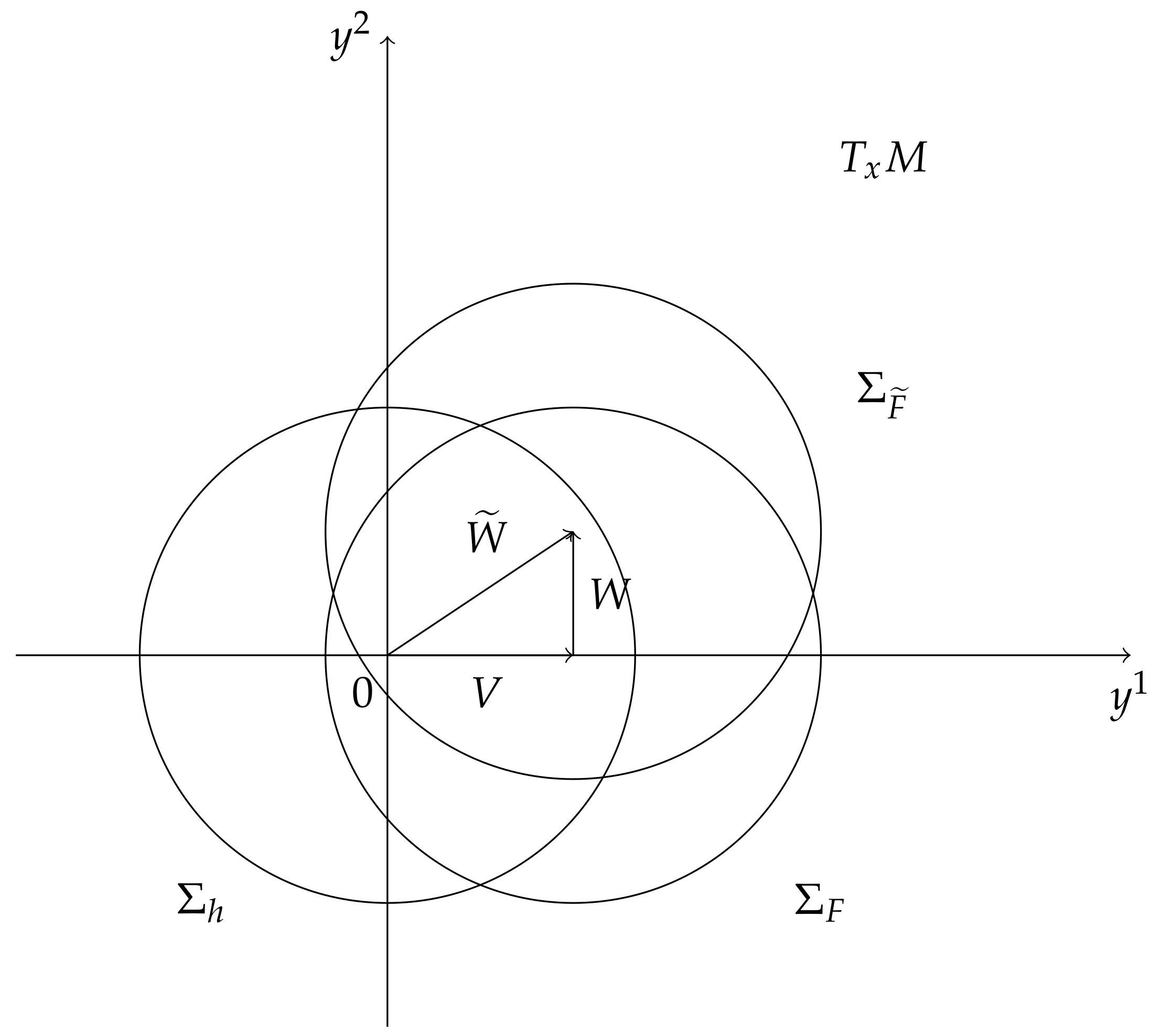
  • Observe that we actually perform a rigid translation of the Riemannian indicatrix Σ h by W ˜ , which is actually equivalent to translating Σ h by V followed by the translation of Σ F by W (see Remark 2).
  • Observe that the Randers metric given by (29) on the topological cylinder R × S 1 is rotational invariant, hence ( M , α ˜ + β ˜ ) is a Finslerian surface of revolution. This type of Randers metrics are called Randers rotational metrics. Indeed, let us denote m F ( r ) : = F ( θ | ( r , θ ) ) . Observe that in the case A ( r ) is an odd or even function, the function m F ( r ) is an even function such that m F ( 0 ) > 0 .
Theorem 4 implies
Theorem 6.
Let ( M , h ) be the topological cylinder R × S 1 with the Riemannian metric h = d r 2 + m 2 ( r ) d θ 2 and W ˜ = A ( r ) r + B θ , A 2 ( r ) + B 2 m 2 ( r ) < 1 . If we denote by F ˜ = α ˜ + β ˜ the solution of Zermelo’s navigation problem for ( M , h ) and W ˜ , then the followings are true.
 (i)
The F ˜ -unit speed geodesics P ( t ) are given by
P ( t ) = ( r ( s ( t ) ) , θ ( s ( t ) ) + B · s ( t ) ) ,
where γ ( s ) = ( r ( s ) , θ ( s ) ) is α-unit speed geodesic and t = t ( s ) is the parametric change t = 0 s F ( γ ( τ ) , γ ˙ ( τ ) ) d τ .
 (ii)
The point q = P ( l ) is conjugate to P ( 0 ) = p along the F ˜ -geodesic P if and only if q ^ = ( r ( q ) , θ ( q ) B · l ) is conjugate to p with respect to α along the α-geodesic from p to q ^ .
 (iii)
The point q ^ C u t α ( p ) is an α-cut point of p if and only if q = ( r ( q ^ ) , θ ( q ^ ) + B · l ) C u t F ˜ ( p ) , where l = d F ˜ ( p , q ) .
Proof of Theorem 6.
First of all, observe that V = A ( r ) r and W = B θ satisfy conditions (i), (ii) in the hypothesis of Theorem 4.
Indeed, since ( M , h ) is surface of revolution and V = ( A ( r ) , 0 ) , it results that η = A ( r ) d r is closed form, hence (24) is satisfied.
Moreover, W = B θ is obviously Killing field with respect to h, and it is trivial to see that [ V , W ] = A ( r ) r , B θ = 0 .
The statements (i)–(iii) follow now from Theorem 4 and the fact that the flow of W = B θ is just φ t ( r , θ ) = ( r , θ + B t ) for any ( r , θ ) M , t R .
In this case, β ( W ) = 0 , hence F ( W ) = F ( W ) = α ( W ) < 1 , hence (iii) is necessary and sufficient condition. □
We have reduced the geometry of the Randers type metric ( M , F ˜ ) to the geometry of the Riemannian manifold ( M , α ) , obtained from ( M , h ) by (30).
Example 1.
Let us observe that there are many cylinders ( M , h ) and winds W ˜ satisfying the condition A 2 ( r ) + B 2 m 2 ( r ) < 1 in Theorem 6.
For instance, let us consider the topological cylinder R × S 1 with the Riemannian metric h = d r 2 + m 2 ( r ) d θ 2 defined using the warp function m ( r ) = e r 2 .
Consider the smooth function A : R 1 2 , 1 2 , A ( r ) = 1 2 r r 2 + 1 and any constant B 1 2 , 1 2 .
Then, A 2 ( r ) + B 2 m 2 ( r ) < 1 2 + B 2 m 2 ( r ) 1 2 + B 2 < 1 .
In this case, F ˜ = α ˜ + β ˜ is given by
( a ˜ i j ) = 1 Λ 2 1 B 2 e 2 r 2 B 2 r e 2 r 2 r 2 + 1 B 2 r e 2 r 2 r 2 + 1 1 2 ( r 2 + 2 ) e 2 r 2 r 2 + 1 , ( b ˜ i ) = 1 Λ 1 2 r r 2 + 1 B e 2 r 2 ,
where Λ = 1 2 r 2 + 2 r 2 + 1 B 2 e 2 r 2 .
Observe that F = α + β is given by
( a i j ) = 1 λ 1 0 0 λ e 2 r 2 , ( b i ) = 1 λ 1 2 r r 2 + 1 0 ,
where λ = 1 2 r 2 + 2 r 2 + 1 .
Moreover, we have
Corollary 2.
 (i)
With notations in Theorem 6, if there exist a smooth function A : R ( 1 , 1 ) and a constant B such that A 2 ( r ) + B 2 m 2 ( r ) < 1 and if G α ( r ) < 0 everywhere, then the α-cut locus and the F = α + β cut locus of a point p M is the opposite meridian to the point p.
Moreover, the F ˜ = α ˜ + β ˜ cut locus of p = ( r 0 , θ 0 ) is the deformed opposite meridian by the flow of the vector field W = B θ .
 (ii)
With the notations in Theorem 6, if there exist a smooth function A : R ( 1 , 1 ) and a constant B such that A 2 ( r ) + B 2 m 2 ( r ) < 1 , G α ( r ) is decreasing along any half meridian and G α 0 , then the α-cut locus and the F-cut locus of a point p = ( r 0 , θ 0 ) are given as in Theorem 5.
Moreover, the F ˜ -cut locus of p is obtained by the deformation of the cut locus described in Theorem 5 by the flow of W = B θ .
Proof Corollary 2.
(i)
It follows from Proposition 6 and Theorem 6.
(ii)
Likewise, it follows by combining Proposition 6 and Remark 8, part 1.
 □
Remark 10.
It is not trivial to obtain concrete examples satisfying conditions (I) and (II) in Corollary 2 in the case A not constant. We conjecture that such examples exist leaving the concrete construction for a forthcoming research. The case A = constant is treated below.

4.4. The Case Special W ˜ = A r + B θ

Consider the case W ˜ = ( W ˜ 1 , W ˜ 2 ) = ( A , B ) , where A and B are constants, on the topological cylinder M = { ( r , θ ) : r R , θ [ 0 , 2 π ) } . Here, m : R [ 0 , ) is an even bounded function such that m 2 < 1 A 2 B 2 , | A | < 1 , B 0 .
Proposition 6 and Theorem 6 can be easily rewritten for this case by putting A ( r ) = A = constant. We will not write them again here.
Instead, let us give some special properties specific to this case. A straightforward computation gives:
Proposition 7.
Let ( M , h ) be the Riemannian metric of the cylinder R × S 1 , and let W ˜ = A r + B θ , with A , B real constants such that m 2 < 1 A 2 B 2 , | A | < 1 , B 0 .
Then, the followings are true.
 (i)
The Gauss curvatures G h and G α of ( M , h ) and ( M , α ) , respectively, are proportional, i.e.,
G h ( r ) = 1 λ 2 G α ( r ) ,
where α is the Riemannian metric obtained in the solution of the Zermelo’s navigation problem for ( M , h ) and V = A r .
 (ii)
The geodesic flows S h and S α of ( M , h ) and ( M , α ) , respectively, satisfy
S h = S α + Δ ,
where Δ = A 2 m m ( y 2 ) 2 y 1 is the difference vector field on T M endowed with the canonical coordinates ( r , θ ; y 1 , y 2 ) .
Indeed, observe that since h = d r 2 + m 2 ( r ) d θ 2 and α 2 = 1 λ 2 d r 2 + m 2 ( r ) λ d θ 2 , with λ = 1 A 2 , the non-vanishing Christoffel symbols γ j k i and Γ α j k i of h and α are
γ 22 1 = m m , γ 12 2 = m m , a n d Γ α 22 1 = m m + A 2 m m , Γ α 12 2 = m m ,
respectively. The Gauss curvatures of h and α follows by direct computation using the usual formulas and (i) follows.
From here it also follows that the geodesic spray coefficients of h and α are
G h 1 = γ j k 1 y j y k = m m ( y 2 ) 2 , G h 2 = γ j k 2 y j y k = 2 m m y 1 y 2 a n d G α 1 = Γ α j k 1 y j y k = ( m m + A 2 m m ) ( y 2 ) 2 , G α 2 = Γ α j k 2 y j y k = 2 m m y 1 y 2 ,
respectively, hence the geodesic spray coefficients of h and α are
S h = y i x i G h i y i = y 1 x 1 + y 2 x 2 + m m ( y 2 ) 2 y 1 2 m m y 1 y 2 y 2 a n d S α = y i x i G α i y i = y 1 x 1 + y 2 x 2 + m m ( y 2 ) 2 y 1 2 m m y 1 y 2 y 2 A 2 m m ( y 2 ) 2 y 1 ,
respectively, hence the formula for Δ in (ii). Here, we denote ( r , θ ; y 1 , y 2 ) the canonical coordinates of T ( R × S 1 ) .
Moreover, from Theorem 6 we have
Theorem 7.
In this case, if ( M , h ) is a Riemannian metric on the cylinder M = R × S 1 with bounded warp function m ( r ) < 1 A 2 B , where A , B are constants, | A | < 1 , B 0 , and wind W ˜ = A r + B θ , then the following hold good.
 (I)
If G h ( r ) < 0 everywhere, then
 (i)
the α-cut locus of a point p is the opposite meridian.
 (ii)
the F-cut locus of a point p is the opposite meridian, where F = α + β ,
( a i j ) = 1 λ 2 1 0 0 λ m 2 ( r ) , ( b i ) = 1 λ A 0 ,
and λ : = 1 V h 2 = 1 A 2 > 0 ,
 (iii)
the F ˜ -cut locus of a point p is the twisted opposite meridian by the flow action φ t ( r , θ ) = ( r , θ + B t ) .
 (II)
With the notations in Theorem 6 let us assume that ( M , h ) has Gaussian curvature satisfying G h ( r ) is decreasing along any half meridian [ 0 , ) and G h ( 0 ) 0 . Then, in this case, the cut locus of F ˜ = α ˜ + β ˜ is a subarc of the opposite meridian is of the opposite parallel deformed by the flow of W = B θ .
Example 2.
There are many examples satisfying this theorem. For instance, the choice m ( r ) = e r 2 1 gives G h ( r ) = 4 r 2 + 2 which is decreasing on [ 0 , ) and G h ( 0 ) = 2 > 0 . Any choice of constants A , B such that 1 < 1 A 2 B , i.e., A 2 + B 2 < 1 is suitable.
Remark 11.
A similar study can be done for the case B = 0 .
Remark 12.
The extension to the Randers case of the Riemannian cylinders of revolution and study of their cut loci [14] can be done in a similar manner.

5. Conclusions

Finsler structures are more general than the Riemannian ones in the sense that the lengths of opposite vectors (for instance X and X ) are not equal, the distance between two points is not symmetric, and the geodesics are not reversible. These basic differences induce other differences in the study of the conjugate and cut loci, respectively. Despite of the difficulties in studying the geodesics theory on an arbitrary Finsler manifold, we have shown that in the case of a Finsler surface of revolution, things simplify. Especially in the Randers case, we are able to obtain a quite detailed description of geodesics, their local and global behaviour, conjugate and cut loci due to the Zermelo’s navigation description of Randers spaces. Nevertheless, we have shown that the control of all these geometrical objects is possible in a more general case than the classical Killing wind case appearing in [18], for example.

Author Contributions

Conceptualization, R.H. and S.V.S.; supervision, R.H. and S.V.S.; writing—original draft, R.H. and S.V.S.; writing—review and editing, R.H. and S.V.S. All authors have read and agreed to the published version of the manuscript.

Funding

The second author is partially supported by the JSPS grant number 20K03595.

Acknowledgments

We express our gratitude to H. Shimada for continuous support. We thanks to V. Matveev for useful discussion and to M. Tanaka for bringing this topic to our attention. We are also indebted to the anonymous referees whose criticism helped us to improve the exposition.

Conflicts of Interest

The authors declare no conflict of interest.

References

  1. Bao, D.; Chern, S.S.; Shen, Z. An Introduction to Riemann Finsler Geometry; Graduate Texts in Mathematics; Springer: New York, NY, USA, 2000. [Google Scholar]
  2. Bao, D. On two curvature-driven problems in Riemann-Finsler geometry. Adv. Stud. Pure Math. 2007, 48, 19–71. [Google Scholar]
  3. Bryant, R. Projectively flat Finsler 2-spheres of constant flag curvature. Sel. Math. 1997, 3, 161–203. [Google Scholar] [CrossRef] [Green Version]
  4. Myers, S.B. Connections between differential geometry and topology I. Duke Math. J. 1935, 1, 376–391. [Google Scholar] [CrossRef]
  5. Buchner, M. Simplicial structure of the real analytic cut locus. Proc. Am. Math. Soc. 1977, 64, 118–121. [Google Scholar] [CrossRef]
  6. Buchner, M. The structure of the cut locus in dimension less than or equal to six. Compos. Math. 1978, 37, 103–119. [Google Scholar]
  7. Gluck, H.; Singer, D. Scattering of geodesic fields I. Ann. Math. 1978, 108, 347–372. [Google Scholar] [CrossRef]
  8. Shiohama, K.; Shioya, T.; Tanaka, M. The Geometry of Total Curvature on Complete Open Surfaces; Cambridge Tracts in Mathematics 159; Cambridge University Press: Cambridge, UK, 2003. [Google Scholar]
  9. Itoh, J.; Sabau, S.V. Riemannian and Finslerian spheres with fractal cut loci. Diff. Geom. Its Appl. 2016, 49, 43–64. [Google Scholar] [CrossRef] [Green Version]
  10. Hama, R.; Chitsakul, P.; Sabau, S.V. The geometry of a Randers rotational surface. Publ. Math. Debr. 2015, 87, 473–502. [Google Scholar] [CrossRef] [Green Version]
  11. Hama, R.; Kasemsuwan, J.; Sabau, S.V. The cut locus of a Randers rotational 2-sphere of revolution. Publ. Math. Debr. 2018, 93, 387–412. [Google Scholar] [CrossRef]
  12. Kopacz, P. On generalization of Zermelo navigation problem on Riemannian manifolds. Int. J. Geom. Methods Mod. Phys. 2019, 16, 1950058. [Google Scholar] [CrossRef]
  13. Chitsakul, P. The structure theorem for the cut locus of a certain class of cylinders of revolution I. Tokyo J. Math. 2014, 37, 473–484. [Google Scholar] [CrossRef] [Green Version]
  14. Chitsakul, P. The structure theorem for the cut locus of a certain class of cylinders of revolution II. Tokyo J. Math. 2015, 38, 239–248. [Google Scholar] [CrossRef] [Green Version]
  15. Zermelo, E. Über das Navigationsproblem bei ruhender oder veränderlicher Windverteilung. Z. Angew. Math. Mech. 1931, 11, 114–124. [Google Scholar] [CrossRef]
  16. Shen, Z. Finsler metrics with K=0 and S=0. Canad. J. Math. 2003, 55, 112–132. [Google Scholar] [CrossRef]
  17. Bao, D.; Robles, C.; Shen, Z. Zermelo navigation on Riemannian manifolds. J. Differ. Geom. 2004, 66, 377–435. [Google Scholar] [CrossRef]
  18. Robles, C. Geodesics in Randers spaces of constant curvature. Trans. Amer. Math. Soc. 2007, 359, 1633–1651. [Google Scholar]
  19. Sabau, S.V.; Shibuya, K.; Shimada, H. Metric structures associated to Finsler metrics. Publ. Math. Debr. 2014, 84, 89–103. [Google Scholar] [CrossRef]
  20. Innami, N.; Nagano, T.; Shiohama, K. Geodesics in a Finsler surface with one-parameter group of motions. Publ. Math. Debr. 2016, 89, 137–160. [Google Scholar] [CrossRef]
  21. Hrimiuc, D.; Shimada, H. On the L-duality between Lagrange and Hamilton manifolds. Nonlinear World 1996, 3, 613–641. [Google Scholar]
  22. Miron, R.; Hrimiuc, D.; Shimada, H.; Sabau, S.V. The Geometry of Hamilton and Lagrange Spaces; Fundamental Theories of Physics; Kluwer Academic Publishers Group: Dordrecht, The Netherlands, 2001. [Google Scholar]
  23. Foulon, P.; Matveev, V.S. Zermelo deformation of Finsler metrics by Killing vector fields. Electron. Res. Announc. Math. Sci. 2018, 25, 1–7. [Google Scholar] [CrossRef] [Green Version]
Figure 1. Randers metrics: a rigid displacement of an ellipse.
Mathematics 08 02047 g001
Figure 2. The two steps Zermelo’s navigation.
Mathematics 08 02047 g002
Figure 3. The h-indicatrix, F 1 -indicatrix and F-indicatrix.
Mathematics 08 02047 g003
Figure 4. Riemannian and Finsler geodesics in Zermelo’s navigation problem.
Mathematics 08 02047 g004
Figure 5. The angle ϕ between γ ˙ and a meridian for a cylinder of revolution.
Mathematics 08 02047 g005
Figure 6. The two steps Zermelo’s navigation.
Mathematics 08 02047 g006
Publisher’s Note: MDPI stays neutral with regard to jurisdictional claims in published maps and institutional affiliations.

