Comparison between Single and Multi-Objective Evolutionary Algorithms to Solve the Knapsack Problem and the Travelling Salesman Problem

Abstract

One of the main components of most modern Multi-Objective Evolutionary Algorithms (MOEAs) is to maintain a proper diversity within a population in order to avoid the premature convergence problem. Due to this implicit feature that most MOEAs share, their application for Single-Objective Optimization (SO) might be helpful, and provides a promising field of research. Some common approaches to this topic are based on adding extra—and generally artificial—objectives to the problem formulation. However, when applying MOEAs to implicit Multi-Objective Optimization Problems (MOPs), it is not common to analyze how effective said approaches are in relation to optimizing each objective separately. In this paper, we present a comparative study between MOEAs and Single-Objective Evolutionary Algorithms (SOEAs) when optimizing every objective in a MOP, considering here the bi-objective case. For the study, we focus on two well-known and widely studied optimization problems: the Knapsack Problem (KNP) and the Travelling Salesman Problem (TSP). The experimental study considers three MOEAs and two SOEAs. Each SOEA is applied independently for each optimization objective, such that the optimized values obtained for each objective can be compared to the multi-objective solutions achieved by the MOEAs. MOEAs, however, allow optimizing two objectives at once, since the resulting Pareto fronts can be used to analyze the endpoints, i.e., the point optimizing objective 1 and the point optimizing objective 2. The experimental results show that, although MOEAs have to deal with several objectives simultaneously, they can compete with SOEAs, especially when dealing with strongly correlated or large instances.

1. Introduction

Evolutionary Algorithms (EAs) [1] were initially developed for unconstrained Single-Objective Optimization Problems (SOPs). However, extensive research has been conducted to adapt them to other types of problems. In recent years, many Multi-Objective Evolutionary Algorithms (MOEAs) have been proposed in the literature [2,3] to adapt EAs to dealing with Multi-Objective Optimization Problems (MOPs). One of the main components of most modern MOEAs is the ability to maintain genetic diversity within a population of individuals [4]. Maintaining proper diversity is decisive for the behavior of EAs, since a loss of diversity could lead to premature convergence, which is a frequent drawback, especially for single-objective optimization. Most MOEAs implicitly manage diversity by considering the objective function space [5] and, in some cases, the decision variable space. Several mechanisms have been proposed in the literature to deal with the above, such as fitness sharing [6], clustering [7], and entropy [8], among others [4]. Promoting diversity is a key feature of an efficient and reliable MOEA. In fact, it is an intrinsic component in many MOEAs. Because of this, some authors have claimed that the application of MOEAs might be useful when dealing with single-objective problems. Furthermore, several theoretical and empirical studies have shown that multi-objective optimizers can even provide better solutions than single-objective optimizers [4,9,10,11].

MOEAs have been applied to SOPs using various guidelines. Usually, the mechanisms proposed in the literature for solving SOPs by means of MOEAs consist of transforming the original SOP into a MOP so that MOEAs can be applied to the transformed problem. This transformation can be done by either replacing the original objective with a set of new objectives, or by adding new, additional objectives to the original one [4,12]. Among these approaches, the best known and most widespread in the literature are: transforming constraints into objectives [13], considering diversity as an explicit objective function [14] and multiobjectivization schemes, which transform a SOP into a MOP by modifying its fitness landscape [12]. In any case, these new objectives are included in order to promote the exploration of different regions, since multi-objective approaches try to simultaneously optimize several objectives. This might make it possible to escape from sub-optimal regions, thus providing a suitable balance between exploration and exploitation. The analysis presented in [15] lists the benefits of using additional objectives, named helper-objectives. The main ones are [12]: avoiding stagnation in local optima and maintaining diversity within a population.

In this paper, we present a comparative study of MOEAs and SOEAs when both types of schemes are separately applied to optimize each objective function of a bi-objective optimization problem. The study is not intended to provide a novel algorithm or to compare a new proposal with state-of-the-art algorithms. The main goal of this work is to investigate the effectiveness—or at least the opportunities—of applying multi-objective approaches to single-objective optimization. This study relies on comparisons of standard MOEAs and some general SOEAs when they seek to optimize—independently—every objective in a bi-objective problem. In this study, we consider the Knapsack Problem [16] and the Travelling Salesman Problem [17]. Both problems have been considered in numerous theoretical and experimental studies in the literature, so many effective solvers are known to perform successfully for a wide range of benchmarks.

Although there are many contributions that have been made in the field of mathematical optimization, in this work we are interested in the analysis of a particular set of approximated algorithms—named evolutionary algorithms—for both, single and multi-objective formulations of the problems. For this reason, our literature review deepens the field of evolutionary computation and not in other research areas that could also have great impact and interest nowadays. As an alternative, some experts have advocated for pushing further the integration of machine learning and combinatorial optimization [18]. Some operations research communities are introducing machine learning as a modeling tool for discrete optimization [19] or to extract intuition and knowledge in order to dynamically adapt the optimization process [20]. Despite the existence of such a huge amount of alternatives to face these optimization problems, it is important to note that we are interested in the comparative analysis of single and multi-objective evolutionary algorithms. Thus, the selected optimization problems can be understood as simple use cases for our experimental study.

For the experiments, we have selected an extensive and diverse set of problem instances that consider different features, sizes and complexities. However, all the instances have two optimization objectives, meaning they can be used to apply multi-objective approaches. For the optimization process, three MOEAs and two SOEAs have been analyzed. Each SOEA is applied twice for each problem instance (one for each objective), so that the optimized values for each of the two objectives can be compared to the multi-objective solutions offered by the MOEAs in question. The rest of this paper is organized as follows: Section 2 describes the formulation of the two problems selected for this study, as well as the set of instances solved during the experimental process. Then, Section 3 provides an overview of the approaches—MOEAs and SOEAs— applied during this study. A detailed description of the experimental analysis and some underlying results, as well as their discussion, are presented in Section 4 Finally, the conclusions and some lines for future work are presented in Section 5.

2. Problems: Formulation and Instances

This section presents two well-known problems, the Knapsack Problem (KNP) [16] and the Travelling Salesman Problem (TSP) [17], which we have selected to conduct out experimental study. For each problem, a formulation involving two objectives is described, as well as the corresponding set of instances. Note that all instances presented below are bi-objective instances. This means that all instances have information that allow the calculation of two different objective functions to be carried out. Anyway, for the single-objective approaches, we can use only one of the objectives and discard the other, depending on the objective being analyzed at a particular moment.

2.1. The Bi-Objective Knapsack Problem (BOKNP)

We consider the one-dimensional 0/1 knapsack problem with two objectives, where fractional items are not allowed and each item is available only once. This multi-objective one-dimensional binary knapsack problem can be defined as follows. Given a set of items $J=\{1,\dots ,n\}$, each with an associated weight $w_j\in {\mathbb{N}}^{*}$ and a profit $c_j^k\in {\mathbb{N}}_0$ for each objective $k\in K=\{1,\dots ,p\}$, the problem seeks to select the subset of J whose total weight does not exceed a fixed capacity $W\in {\mathbb{N}}^{*}$, while simultaneously maximizing the accumulated profit according to each objective in K. Mathematically, the problem can be formulated as follows [21]:

$$\begin{array}{l}{\displaystyle \begin{array}{cc}{\displaystyle max{f}_1\left(x\right)}& \sum _{j=1}^n{c}_j^1{x}_j\hfill \\ ⋮& ⋮\hfill \\ {\displaystyle max{f}_p\left(x\right)}& \sum _{j=1}^n{c}_j^p{x}_j\hfill \end{array}}\\ \mathrm{subject}\mathrm{to}\sum _{j=1}^n{w}_j{x}_j\le W,x_j\in \{0,1\}\end{array}$$

(1)

Moreover, and without loss of generality, we assume that $c_j^k\ge 0$ and $w_j\le W:\forall j\in \{1,\dots ,n\},\forall k\in \{1,\dots ,p\}$. Since, in this work, we are interested in a bi-objective formulation of this problem, we let $p=2$, such that the set K contains two functions ($f_1$ and $f_2$) to be optimized, $K=\{1,2\}$.

For this bi-objective knapsack problem, we propose using the subset benchmark “MOKP” data sets available in the MOCOlib project [22]. MOCOlib is a collection of data sets and links for a variety of multi-objective combinatorial optimization problems. In this collection, we found three different sets of instances that are suitable for the bi-objective 0/1 unidimensional knapsack problem defined herein.

The data files themselves contain a description of the instances. Table 1 is attached in order to summarize the main features of the different sets of instances as well as their original references. Some of the key points for each data set are briefly broken down here:

1.

Data set 1A: consists of five data files (instances) for the bi-objective 0/1 unidimensional knapsack problem. The values for the profits and weights have been uniformly generated. The number of items in the instances range from 50 to 500. The tightness ratio (Equation (2)) is in the range $[0.11,0.92]$.

$$\begin{array}{c}{\displaystyle \begin{array}{cc}\hfill {\displaystyle }& r=\frac{W}{{\sum }_{i=1}^n{w}_i}\hfill \end{array}}\end{array}$$

(2)

2.

Data set 1B: consists of 40 data files (instances) corresponding to the 10 bi-objective 0/1 unidimensional knapsack problems. Every instance has a tightness ratio $r=0.5$. For each problem, four variants (class A, B, C and D) are given:

• 1B/A: the weights and profits are uniformly distributed within the range $[1,100]$.
• 1B/B: these instances are created starting from data set 1B/A by defining the objectives in reverse order.
• 1B/C: the profits are generated with plateaus of values of length $\le 0.1\times n$.
• 1B/D: these instances are created starting from data set 1B/C by defining the objectives in reverse order.

3.

Data set 2: consists of 50 data files (instances) that also correspond to the bi-objective 0/1 unidimensional knapsack problem. For each data set the value for W is computed as the nearest integer value of $(P/100){\sum }_{j=1}^n{w}_j$ (where P is a percentage of ${\sum }_{j=1}^n{w}_j$). All these instances have a tightness ratio $r=0.5$. Two types of correlated instances (WEAK and STRONG), as well as uncorrelated instances (UNCOR) were generated as follows [21]:

• UNCOR: 20 uncorrelated instances of 50 items. The profit vectors $c_j^1$, $c_j^2$ and the weight vector $w_j$ are uniformly generated at random in the range $[1,300]$ for ten items, while for the remaining ones the range $[1,1000]$ is considered.
• WEAK: 15 weakly correlated instances ranging in size from 50 to 1000 items, where $c_j^1$ is correlated with $c_j^2$, i.e., $c_j^2\in [111,1000]$, and $c_j^1\in [c_j^2-100,c_j^2+100]$. The weight values $w_j$ are uniformly generated at random in the range $[1,1000]$.
• STRONG: 15 strongly correlated instances with the number of items ranging between 50 and 1000. The weights $w_j$ are uniformly generated at random and are correlated with $c_j^1$, i.e., $w_j\in [1,1000]$, and $c_j^1=w_j+100$. The value of $c_j^2$ is uniformly generated at random in the range $[1,1000]$.

Table 1. Bi-objective KNP instances. The instance number (s), the number of items (n) and tightness ratio (r) refer to the parameters of the instances.

Set	Source	Name	Parameters
Set 1A	Gandibleux and Freville [23]	2KNP50-r	$n=50;r\in \{0.11,0.50,0.92\}$
		2KNP100-50	$n=100;r=0.50$
		2KNP500-41	$n=500;r=0.41$
Set 1B/A	Visée et al. [24]	2KNPn-1A	$n\in \{100,200,300,400,500\};r=0.5$
Set 1B/B,C,D	Degoutin and Gandibleux [25]	2KNPn-1B	$n\in \{100,200,300,400,500\};r=0.5$
		2KNPn-1C	$n\in \{100,200,300,400,500\};r=0.5$
		2KNPn-1D	$n\in \{100,200,300,400,500\};r=0.5$
Set 2 (UNCORR)	Captivo et al. [21]	F5050Ws	$s\in \{01,02,03,\dots ,10\};n=50;r=0.5$
		K5050Ws	$s\in \{01,02,03,\dots ,10\};n=50;r=0.5$
Set 2 (WEAK)	Captivo et al. [21]	W4C50W01	$n=50;r=0.5$
		W4100W1	$n=100;r=0.5$
		4WnW1	$n\in \{150,200,\dots ,1000\};r=0.5$
Set 2 (STRONG)	Captivo et al. [21]	S1C50W01	$n=50;r=0.5$
		S1nW1	$n\in \{100,150,200\};r=0.5$
		1SnW1	$n\in \{250,300,\dots ,1000\};r=0.5$

Table 1. Bi-objective KNP instances. The instance number (s), the number of items (n) and tightness ratio (r) refer to the parameters of the instances.

Set	Source	Name	Parameters
Set 1A	Gandibleux and Freville [23]	2KNP50-r	$n=50;r\in \{0.11,0.50,0.92\}$
		2KNP100-50	$n=100;r=0.50$
		2KNP500-41	$n=500;r=0.41$
Set 1B/A	Visée et al. [24]	2KNPn-1A	$n\in \{100,200,300,400,500\};r=0.5$
Set 1B/B,C,D	Degoutin and Gandibleux [25]	2KNPn-1B	$n\in \{100,200,300,400,500\};r=0.5$
		2KNPn-1C	$n\in \{100,200,300,400,500\};r=0.5$
		2KNPn-1D	$n\in \{100,200,300,400,500\};r=0.5$
Set 2 (UNCORR)	Captivo et al. [21]	F5050Ws	$s\in \{01,02,03,\dots ,10\};n=50;r=0.5$
		K5050Ws	$s\in \{01,02,03,\dots ,10\};n=50;r=0.5$
Set 2 (WEAK)	Captivo et al. [21]	W4C50W01	$n=50;r=0.5$
		W4100W1	$n=100;r=0.5$
		4WnW1	$n\in \{150,200,\dots ,1000\};r=0.5$
Set 2 (STRONG)	Captivo et al. [21]	S1C50W01	$n=50;r=0.5$
		S1nW1	$n\in \{100,150,200\};r=0.5$
		1SnW1	$n\in \{250,300,\dots ,1000\};r=0.5$

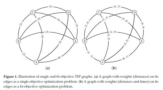
2.2. The Bi-Objective Travelling Salesman Problem (BOTSP)

In this work we consider a generalization of the classical Travelling Salesman Problem (TSP), which is defined as follows. Given a complete graph—or fully connected network—$G=(V,E)$ with vertex set V (cities), edge set E (paths between any two cities $i,j\in \{1,\dots ,n\})$, and edge values $c_{ij}^k$ with $k\in K=\{1,\dots ,p\}$ (objective cost—it could be distance, time, energy, etc.—between city i and city j), the problem is to find the Hamiltonian path [26] (tour), which is a single and cyclic circuit, along the edges of G, such that each vertex (city) is visited exactly once and the total tour for each objective k, defined as the sum of costs $c_{ij}^k$, is minimized. A more detailed description of this multi-objective formulation of TSP can be found in [27].

Given a graph $G=(V,E)$, where $V=\{1,2,\dots ,n\}$ and $E=\{(i,\pi \left(i\right)),i\in V\}$, ${\Pi }_n$ denotes the set of all possible permutations of n cities. For a permutation $\pi \in {\Pi }_n$, $\pi \left(i\right)$ represents the city that follows city i on the tour represented by permutation $\pi$. A permutation whose graph is a Hamiltonian path is called a cyclic permutation. We denote by ${\Pi }^c$ the set of all cyclic permutations of n cities. Therefore, a TSP tour can be represented by a permutation $\pi =(\pi \left(1\right),\dots ,\pi \left(n\right))\in {\Pi }^c$. Thus, the formulation of the multi-objective TSP is given by:

$$\begin{array}{c}{\displaystyle \begin{array}{cc}\hfill {\displaystyle \underset{\pi \in {\Pi }^c}{min}\sum _{i=1}^{n-1}{c}_{\pi \left(i\right),\pi (i+1)}^k+c_{\pi \left(n\right),\pi \left(1\right)}^k}& k=\{1,\dots ,p\}\hfill \end{array}}\end{array}$$

(3)

Since in this work we are interested in multi-objective problems with two optimization objectives, we have considered the bi-objective TSP formulation. Thus, the general Equation (3) is considered, in which $k=\{1,2\}$. Figure 1 is provided to better clarify the differences between a single and a bi-objective formulation of the TSP. Figure 1a illustrates a single-objective formulation of the TSP where there is only one set of costs (one for each edge), thus defining a single optimization function. As a result, the single-objective formulation of the TSP consists of a list of n cities and a set of costs—a single cost for each pair of cities—which are all stored in a cost matrix D with elements $c_{ij}$, with $i,j\in \{1,\dots ,n\}$, and diagonal elements $c_{ii}=0$. However, Figure 1b shows the differences between a single and a bi-objective instance of the TSP. As shown in the example, a bi-objective formulation considers instances with two different costs for each edge: one cost for objective 1 and another for objective 2. Instead of having a single cost matrix, in a multi-objective formulation, we need to manage a cost matrix for each objective function considered.

For this bi-objective formulation of the problem, we need a suitable set of problem instances: different types, sizes and costs between cities. Two types of instances are selected for the experimental study that is presented in this work. First, in the Euclidean instances, the costs between edges correspond to the Euclidean distance between two points on a plane, randomly sampled from a uniform distribution. Meanwhile, in the clustered instances, the points are randomly clustered on a plane, and the costs between edges correspond to the Euclidean distance. Then, the bi-objective instances are obtained by combining a pair of single-objective instances. Table 2 shows the information for the 19 problem instances of symmetric bi-objective TSPs with 100, 300 and 500 cities (these instances are available at http://www-desir.lip6.fr/~lustt/). These instances have been used in several related works [28,29,30], so they have been successfully solved in the literature. In fact, their exact fronts were already published by K. Florios (optimal fronts are available at https://sites.google.com/site/kflorios/motsp). More details on the selected instances are given below:

• The TSPLIB Euclidean Instances [31] (files with prefix kro, from the authors Krolak/Felts/Nelson) consist of 13 instances with two objectives which are generated on the basis of the single-objective TSP instances from TSPLIB [32] (Library of Traveling Salesman Problems). The TSPLIB is a library of sample instances for the TSP (and related problems) from various sources and with different features.
• The DIMACS Clustered Instances [33] (files with prefix clus) are three instances that have been created using the random instance generator available from the 8th DIMACS implementation challenge site (the generator is available at http://dimacs.rutgers.edu/archive/Challenges/TSP/index.html).
• The DIMACS Euclidean Instances [30] (files with prefix eucl) are a set of three instances which were also generated using the DIMACS code.

Table 2. Bi-objective TSP instances.

Name	Origin	Type	Source	Num. of Variables	Combinations
clusABn	DIMACS	Clustered	Lust et al. [33]	$n\in \{100,300,500\}$	clusAn and clusBn
euclABn	DIMACS	Euclidean	Paquete et al. [30]	$n\in \{100,300,500\}$	euclAn and euclBn
kroABn	TSPLIB	Euclidean	Paquete et al. [30]	$n\in \{100,150,200,300,400,500,750,1000\}$	kroAn and kroBn
kroACn					kroAn and kroCn
kroADn					kroAn and kroDn
kroBCn	TSPLIB	Euclidean	Paquete et al. [30]	$n\in \{100\}$	kroBn and kroCn
kroBDn					kroBn and kroDn
kroCDn					kroCn and kroDn

Table 2. Bi-objective TSP instances.

Name	Origin	Type	Source	Num. of Variables	Combinations
clusABn	DIMACS	Clustered	Lust et al. [33]	$n\in \{100,300,500\}$	clusAn and clusBn
euclABn	DIMACS	Euclidean	Paquete et al. [30]	$n\in \{100,300,500\}$	euclAn and euclBn
kroABn	TSPLIB	Euclidean	Paquete et al. [30]	$n\in \{100,150,200,300,400,500,750,1000\}$	kroAn and kroBn
kroACn					kroAn and kroCn
kroADn					kroAn and kroDn
kroBCn	TSPLIB	Euclidean	Paquete et al. [30]	$n\in \{100\}$	kroBn and kroCn
kroBDn					kroBn and kroDn
kroCDn					kroCn and kroDn

3. Optimization Approaches

This section provides a description of all the algorithmic approaches selected, and thus considered in the experimental study. We also attempt to justify the selection and design decisions made.

3.1. Multi-Objective Evolutionary Algorithms

Evolutionary Multi-Objective Optimization (EMO) [34] is a collection of research, applications and algorithms in the field of Multi-Objective Optimization (MO) paradigms using Evolutionary Algorithms (EAs). In the related literature, several Multi-Objective Evolutionary Algorithms (MOEAs) have been proposed for solving MOPs, and these can be classified based on different features. A widely accepted classification for MOEAs is one that considers the following families:

• Pareto-dominance-based algorithms use the Pareto dominance relationship, where the partner of a non-dominated individual is chosen from among the individuals of the population that it dominates. Some widely known algorithms from this type are: Non-Dominated Sorting Genetic Algorithm II (NSGA-II) [35], Strength Pareto Evolutionary Algorithm 2 (SPEA2) [36] and Pareto Envelope-based Selection Algorithm II (PESA-II) [37].
• Decomposition-based algorithms transform a MOP into a set of SOPs using scalarizing functions. The resulting single-objective problems are then solved simultaneously. Some examples of algorithms that fall under this approach are Multi-Objective Genetic Local Search algorithm (MOGLS) [38], Cellular Multi-Objective Genetic Algorithm (C-MOGA) [39] and Multi-Objective Evolutionary Algorithm based on Decomposition (MOEA/D) [40], as well as their many other variants.
• Indicator-based algorithms use an indicator function to assess the quality of a set of solutions, combining the degree of convergence and/or the diversity of the objective function space with a metric. These algorithms attempt to find the best subset of Pareto non-dominated solutions based on the performance indicator. Their many variants include: Indicator Based-Selection Evolutionary Algorithm (IBEA) [41], S-Metric Selection Evolutionary Multi-Objective Optimization Algorithm (SMS-EMOA) [42], Fast Hypervolume Multi-Objective Evolutionary Algorithm (FV-MOEA) [43] and Many-Objective Metaheuristic Based on R2 Indicator (MOMBI-II) [44].

The No Free Lunch Theorem in optimization [45] states that any algorithm that searches for an optimal cost or fitness solution is not universally superior to any other algorithm. Therefore, for experimental studies, at least one algorithm of each type is usually selected as part of the state of the art. In this work, we apply a Pareto-dominance-based algorithm (NSGA-II), a decomposition-based approach (MOEA/D) and an indicator-based algorithm (SMS-EMOA), which guides the search by means of the hypervolume metric. A brief description of said multi-objective approaches is provided below:

• NSGA-II [35] is a generational genetic algorithm and is one of the most popular multi-objective optimization algorithms, having been widely and successfully applied in many real-world applications. It is one of the first multi-objective algorithms to introduce elitism, i.e., the elites of a population are given the opportunity to be carried to the next generation. It uses a fast non-dominated sorting procedure based on Pareto front ranking in an effort to promote convergence, meaning it emphasizes non-dominated solutions. In addition to the reasons given above, we have selected this algorithm because it uses an explicit diversity preservation mechanism (crowding distance).
• MOEA/D [40] is probably the most representative decomposition-based multi-objective algorithm. It processes a multi-objective problem by decomposing it into a set of single-objective subproblems and then performing a heuristic search in order to optimize—simultaneously and cooperatively—said subproblems. Generally, a MOEA needs to maintain diversity in its population to produce a set of representative solutions. MOEAs, such as NSGA-II, use crowding distances to maintain diversity. In MOEA/D, a MOP is decomposed into a number of scalar optimization subproblems. Different solutions in the current population are associated with different subproblems. The diversity among these subproblems will naturally lead to diversity in the population [40], which could reinforce the rationale for selecting this algorithm in the context of this study.
• SMS-EMOA [42] is an indicator-based algorithm that implements a special selection operator that combines the hypervolume metric with the concept of Pareto dominance. Since the hypervolume is a measure frequently applied for comparing the results of MOEAs, the underlying idea is to explicitly manage and maximize the dominated hypervolume within the optimization process. Hypervolume, which is also used for comparison purposes, measures convergence, as well as diversity. The SMS-EMOA keeps a population of non-dominated and dominated individuals at a constant size. Keeping only non-dominated individuals might lead to small or even single-membered populations, and thus to a crucial loss of diversity. To avoid losing diversity, defining a lower bound for the population size was suggested in [42]. These are the reasons that make SMS-EMOA a good candidate for this study, especially to test the effectiveness of the diversity of this algorithm to improve results in MOPs.

3.2. Single-Objective Evolutionary Algorithms

In the context of SOEAs, some of the most frequently used approaches are Evolution Strategies (ESs) and Genetic Algorithms (GAs). The main differences between these types of EAs lie in the calculation of the fitness and the application of operators (mutation, recombination and selection). In contrast to GAs, where the main role of the mutation operator is simply to avoid the problem of premature convergence, mutation is the primary operator of ESs. Furthermore, in contrast to GAs, selection in the case of ESs is absolutely deterministic. For the experimental study conducted in this work, we considered the following approaches:

• Generational Genetic Algorithm (gGA) [46]: two parents are selected from the population in order to be crossed, yielding two offspring, which are later mutated and evaluated. These newly generated individuals are placed in an auxiliary population that will replace the current population when it is completely full.
• Steady-State Genetic Algorithm (ssGA) [47]: two parents are selected and crossed, yielding two offspring that are later crossed. Then one of the resulting offspring is mutated. The mutated individual is evaluated and then inserted into the population, usually replacing the worst individual in the population (if the new one is better). Hence, the parents and offspring can co-exist in the population for the next iteration.
• Elitist Evolution Strategy ($\mu$ + $\lambda$) (eES) [48]: the elitist feature allows for the best solution to be always kept. The algorithm starts with a population of size $\mu$. Each generation $\lambda$ of mutated individuals is created from the current population. After the generation of the mutated individuals, there are a total of ($\mu +\lambda$) individuals, including the parents and the new individuals generated from them. From these ($\mu +\lambda$) individuals, the best $\mu$ ones are kept—as parents—for the next generation.
• Non-Elitist Evolution Strategy ($\mu$, $\lambda$) (neES) [48]. in this case the best $\mu$ mutated individuals from among the new generated $\lambda$ are selected as parents for the next generation, i.e., none of the $\mu$ parents survive the next generation, meaning $\lambda \ge \mu$ must hold.

3.3. Comparison of Single and Multi-Objective Approaches

For the comparison we will use the same set of bi-objective instances for the single-objective and multi-objective algorithms here considered. Our aim will be to analyze the objectives independently, i.e., first comparing the values of MOEAs and SOEAs for objective 1 in the whole set of instances considered, and then, in a similar way, by comparing objective 2. The multi-objective approaches directly address the bi-objective instances selected for the KNP and the TSP. The above means that they obtain, at every execution, an extreme—best—value for objective 1, and another extreme—best—value for objective 2. We note that both values—for the two optimization objectives—are obtained at the same time, i.e., in one single execution of the algorithm. However, the single-objective approaches cannot deal with several objectives simultaneously, and therefore, they need to be executed twice: once to optimize objective 1 and another to optimize objective 2.

During the experimental evaluation we will focus on solution quality when comparing the different approaches, i.e., we will not perform any analysis on the execution time for each approach. Due to their stochastic nature, the time complexity analysis of EAs is not an easy task [49]. Many experimental results have been reported on all types of EAs but only a few results have been proved on a theoretical context [50]. Besides, when the complexity analysis is about MOEAs, the development of a theoretical study is even more complicated [51]. Since MOEAs implicitly deal with objectives that are in conflict one with each other, they need to manage a set of trade-off solutions instead of one single (optimal) solution. When tackling MOPs is necessary to distinguish the quality of solutions consisting of multiple objective values. In many MOEAs, it is common to use the concepts of Pareto dominance in order to sort a set of solutions: non-dominated sorting. This sorting procedure aims to divide a solution set into a number of disjoint subsets or ranks, by means of comparing their values of the same objective. After the sorting process, solutions in the same rank are viewed equally important, and solutions in a smaller rank are better than those in a larger rank. Since a wide range of the existing MOEAs have adopted this sorting strategy, they all involve a high computational cost [52]. Some studies have shown that in an approach such as NSGA-II applied to a bi-objective DTLZ1 benchmark problem, the non-dominated sorting consumes more than 70% of the run-time for a population size of 1000 individuals and a maximum number of generations equal to 500 [52]. In our study, the execution times of the multi-objective approaches range from 5 to 10 times greater in comparison to the time required by the two executions–one for each objective–of the corresponding single-objective alternatives. These values depend on the problem (KNP or TSP) and on the instance type or size. When dealing with many-objective optimization problems (three or more objectives) this aspect of efficiency becomes even more critical. Bearing the above in mind, some authors have actively worked on reducing the number of objective functions by eliminating those that are not essential to describe the Pareto-optimal front [53].

4. Experimental Results

As noted in previous sections, for the experimental study we considered the bi-objective KNP and TSP formulations. Moreover, we have described the set of instances that could be used in the context of these formulations. Regarding the type of approaches to apply, as mentioned previously, we are interested in evaluating the possibilities offered by a multi-objective optimization mechanism where we analyze, from the resulting Pareto front, the end points in each objective independently. The optimization approaches compared herein consist of three MOEAs (NSGA-II, MOEA/D, and SMS-EMOA) and two single-objective algorithms (gGA and eES). Note that, initially, we checked the behavior of four single-objective approaches, but two of them (ssGA and neES) were discarded for the exhaustive study presented here. This is because the results output by these algorithms were not at all competitive when compared to the single-objective algorithms finally selected for our comparisons (gGA and eES).

4.1. Parameter Setting

Since our focus is to conduct an experimental comparison between different MOEAs and different SOEAs, it was necessary to carry out an exhaustive process to adjust and analyze the ideal parameters for each algorithm. This section provides all the details on the algorithm configurations and the experimental set-up. It is important to note that all the algorithms were implemented in Java using the jMetal [54] framework (the source code used in the current work, as well as the results and graphics extracted from them, can be found through https://github.com/Tomas-Morph/knp-tsp-journal-mathematic). We also used the irace package [55] to set the automatic parameters in all of the algorithms implemented. For each problem—KNP and TSP—we defined a common solution encoding for all the algorithms implemented. We also decided to apply some standard and basic operators for all the algorithms implemented (and in the same way for all of them). To set the automatic parameters, a personalized adjustment was made for each approach. The set of configuration parameters that were automatically tuned—for each algorithm—are as follows:

• Common operator parameters: mutation and crossover probabilities.
• Algorithm parameters: population sizes and other algorithm-specific parameters.
• Other parameters: selection, crossover, and mutation operators. These parameters were set for each optimization problem, using the same operators for all the single and multi-objective approaches.

As previously indicated, the parameters listed were automatically tuned using the irace package. We first ran irace with the set of input parameters described in

Table 3. Input parameter set for irace auto-configuration.

Input Parameter	Possible Values	NSGA	MOEA/D	SMS-EMOA	gGA	eES
Crossover probability	[0.0, 1.0]	√	√	√	√
Mutation probability	[0.0, 1.0]	√	√	√	√	√
Population size	{10, 20, 50, 100, 200, 300}	√	√	√	√	($\mu$)
Offspring population size	{1, 2, 5, 10, 20, 50, 100, 200, 300}	√			√	($\lambda$)
Selection tournament size	[2, 10]	√		√	√
Hypervolume offset	{10, 20, 50, 100, 200, 500}			√
Neighborhood size	{10, 20, 50, 100}		√
Neighbor select probability	[0.0, 1.0]		√

. For this initial tuning process, we selected a subset of representative instances (different type and sizes) for each problem. The best configuration obtained by this automatic process for each pair problem-algorithm after training for a few hours is shown in

Table 4. Parameter settings for each problem-algorithm pair.

Parameter	KNP					TSP
Encoding	Binary strings					Permutation of integers
Initial solutions	random					random
Mutation operator	Bit-flip					Permutation swap
Crossover operator	Single point					PMX
Selection	Tournament					Tournament
	NSGA	MOEA/D	SMS-EMOA	gGA	eES	NSGA	MOEA/D	SMS-EMOA	gGA	eES
Crossover probability	0.9784	0.9578	0.9512	0.8795	_	0.9843	0.9421	0.9754	0.7895	_
Mutation probability	0.0485	0.0578	0.0358	0.0081	0.2239	0.0163	0.0105	0.0093	0.1116	0.3806
Population size	20	200	20	20	1	20	300	20	20	1
Offspring population size	20	_	_	20	4	20	_	_	100	2
Tournament size	5	_	2	2	_	6	_	2	4	_
Hypervolume offset	_	_	200	_	_	_	_	200	_	_
Neighborhood size	_	20	_	_	_	_	50	_	_	_
Neighbor probability	_	0.8895	_	_	_	_	0.9354	_	_	_

. Considering these parameter settings and in order to achieve statistically significant results, a total of 100 independent runs were executed for each pair (algorithm, problem instance) . In order to statistically support the conclusions, the following statistical testing procedure, which was used in a previous work by the authors [56], was applied to compare the results obtained by the different algorithmic schemes. First, a Shapiro–Wilk test was performed to check whether the values of the results followed a normal (Gaussian) distribution. If so, the Levene test checked for the homogeneity of the variances. If the samples had equal variance, an anova test was done; if not, a Welch test was performed. For non-Gaussian distributions, the non-parametric Kruskal–Wallis test was used. For all the tests, a significance level of $\alpha =0.05$ was considered.

Finally, it is important to note that this study is not intended to offer a comparison of the best-performing algorithms existing in the related literature; the main goal is to analyze the suitability of MOEAs for optimizing single-objective problems.

4.2. Performance

The first set of experiments focused on studying how the algorithms evolved over the course of the executions. Figure 2 and Figure 3 show the evolution—over the number of evaluations—of the mean fitness values for both objectives, for the KNP and TSP, respectively. For this set of experiments, the stopping criterion was set to a large number of function evaluations in order to analyze the convergence of the different approaches studied. This will allow us to set the stopping criteria for all the approaches and instances in subsequent experiments. Finally, we note that this preliminary experiment was not applied to the complete set of instances. Instead, a representative set of instances of different types and sizes was chosen for this preliminary overview.

For the KNP (see Figure 2), we solved a total of nine instances: three instances of size 50 and type UNCOR, three instances of different sizes (300, 600, 900) and type WEAK; and finally three of type STRONG with sizes of 300, 600, and 900. Each set of three instances of the same type (UNCOR, WEAK, or STRONG) is shown in the same row. For each instance, two graphs are shown; at the top, the one for objective 1, and the one for objective 2 below it. Note that, in most cases, the algorithms converge quickly for the initial evaluations. The convergence is only slower for the last instances, i.e., those that are strongly correlated. In general, we can see that all the algorithms yield a sharp increase in solution quality in the early generations of the search. We note that, from approximately $50·{10}^3$ evaluations, the difference in performance remains constant during almost the entire run; as a result, we used this point as the stopping criterion for the next experiment.

Based on the behavior among the different instances, we can state the following. For the uncorrelated instances (first two rows; six graphs in total), we note that the SOEAs dominate for both objectives at all times, although the MOEAs are very close, with a relatively constant difference. However, for the weakly correlated instances, there is no apparent difference among the approaches, although the gGA appears to be slightly superior. Finally, for the strongly correlated instances, we see a clear dominance of the MOEAs for objective 1, with a notable difference between eES and the remaining approaches.

For the TSP (see Figure 3), we notice that the size of the instances is directly related to the behavior of the algorithms: regardless of the type of instance and the objectives, we can differentiate three types of behaviors. For the small instances (with 100 cities), the SOEAs predominate at the beginning of the runs, but we see how NSGA-II always achieves better objective values from the middle of the runs until the end. There is also a noticeable difference in SMS-EMOA, which stagnates from the beginning and fails to converge in all the small instances. However, in the case of medium-size instances (with 300 cities), the SMS-EMOA converges rapidly, together with NSGA-II, exhibiting better performance and surpassing the other algorithms, but only up to $2·{10}^6$ evaluations approximately, where again SMS-EMOA stagnates and is overtaken by SOEAs, which eventually outperforms the other algorithms. For large instances (with 500 cities), once more, SMS-EMOA converges very quickly, in this case accompanied by the other two MOEAs, NSGA-II and MOEA/D, until almost the end of the runs, by which point the SOEAs manage to catch up to the other algorithms. Finally, as concerns the convergence and stagnation of the approaches, we have set the stopping criterion of subsequent experiments to $10·{10}^6$ evaluations, in the case of the TSP.

Since, as we noted, the performance of the MOEAs in the TSP improves with the instance size—especially for SMS-EMOA—we decided to run the two largest instances in the TSP data set. These instances have 750 and 1,000 cities. Figure 4 shows that, for both objectives, MOEAs were able to provide better mean objective values than SOEAs during the entire run. In particular, SMS-EMOA yields the best results, despite being the algorithm that obtained the worst results in the small instances.

4.3. Optimization Behavior

Based on the previous results, for this experiment, we selected $50·{10}^3$ and $10·{10}^6$ function evaluations as the stopping criteria for the KNP and the TSP, respectively. As shown before, since the solutions stop improving by that point for any of the approaches, we can reduce the computational effort without losing generality in the analysis to be performed. Moreover, in this second experiment, we ran the complete set of instances and did the comparison at the end of the executions, once the corresponding stopping criterion was reached. Note that all the algorithms were executed 100 times. In order to compare the results obtained by the multi-objective approaches with those achieved by the single-objective optimizers, we calculated the extreme solutions in the Pareto optimal set, which correspond to the best solution attained for each objective function.

The results shown in

Table 5. Results for KNP instances (objective 1).

	Problem		Multi-Objective									Single-Objective						Test
			NSGAII			MOEA/D			SMSEMOA			GA			ES
			Mean	Median		Mean	Median		Mean	Median		Mean	Median		Mean	Median
Set 1/A	2KP100-50		76.1%	76.1%		81.1%	81.6%		77.3%	77.8%		96.1%	96.3%		93.5%	93.6%		S
	2KP50-11		85.3%	87.5%		89.0%	91.3%		88.9%	88.4%		99.1%	100.0%		96.3%	100.0%		S
	2KP50-50		83.4%	84.9%		92.0%	93.3%		84.0%	85.1%		97.8%	98.3%		95.4%	97.0%		S
	2KP50-92		100.0%	100.0%		100.0%	100.0%		100.0%	100.0%		99.7%	100.0%		98.0%	100.0%		M
	2KP500-41		63.1%	63.4%		63.3%	63.6%		62.4%	62.4%		94.3%	94.4%		88.9%	88.9%		S
Set 1/B	2KP100-1A		70.2%	70.9%		78.4%	78.0%		73.4%	73.5%		96.1%	96.5%		90.7%	90.6%		S
	2KP100-1B		70.1%	70.2%		80.1%	79.8%		72.5%	72.7%		96.7%	96.6%		90.4%	90.8%		S
	2KP100-1C		82.1%	82.6%		85.4%	85.4%		82.6%	83.3%		96.5%	96.6%		93.1%	93.3%		S
	2KP100-1D		83.1%	84.4%		88.0%	87.8%		83.8%	84.8%		96.5%	97.0%		93.4%	93.8%		S
	2KP200-1A		69.6%	70.2%		76.4%	76.6%		71.3%	71.7%		95.7%	95.9%		89.2%	89.6%		S
	2KP200-1B		70.7%	70.7%		76.7%	76.6%		71.6%	71.8%		96.1%	96.4%		90.2%	90.4%		S
	2KP200-1C		65.7%	65.9%		77.2%	77.3%		66.6%	67.3%		96.5%	96.4%		91.0%	91.2%		S
	2KP200-1D		65.2%	65.7%		73.4%	73.7%		67.8%	68.6%		96.4%	96.1%		90.6%	90.8%		S
	2KP300-1A		68.4%	68.4%		73.1%	73.6%		68.7%	69.1%		95.4%	95.4%		89.7%	90.1%		S
	2KP300-1B		69.8%	70.3%		73.7%	73.4%		68.8%	68.9%		95.9%	96.0%		90.5%	90.8%		S
	2KP300-1C		71.1%	71.7%		81.7%	82.2%		71.5%	71.4%		95.2%	95.5%		90.9%	91.2%		S
	2KP300-1D		80.5%	80.3%		82.2%	82.4%		77.3%	77.4%		95.1%	95.3%		89.9%	90.1%		S
	2KP400-1A		68.0%	68.2%		69.4%	69.1%		67.3%	67.7%		95.8%	96.1%		87.8%	87.9%		S
	2KP400-1B		66.2%	65.9%		68.2%	68.0%		66.1%	66.5%		95.5%	95.3%		87.5%	87.4%		S
	2KP400-1C		65.6%	65.2%		69.6%	69.2%		65.4%	65.1%		97.4%	97.6%		85.3%	85.8%		S
	2KP400-1D		55.6%	55.7%		59.2%	59.8%		56.3%	56.4%		96.9%	96.9%		87.1%	87.0%		S
	2KP500-1A		63.9%	64.4%		67.2%	66.8%		63.3%	63.5%		93.4%	93.7%		85.4%	85.4%		S
	2KP500-1B		64.0%	63.8%		66.8%	66.6%		62.7%	62.4%		94.1%	94.2%		86.6%	87.0%		S
	2KP500-1C		75.8%	75.9%		81.4%	81.7%		74.4%	74.7%		95.2%	95.1%		88.3%	88.5%		S
	2KP500-1D		72.3%	72.7%		71.3%	71.4%		69.3%	69.7%		95.0%	94.9%		88.8%	88.3%		S
Set 2/UNCOR	F5050W01		82.9%	84.0%		90.7%	91.9%		80.7%	83.3%		96.9%	97.7%		94.0%	93.7%		S
	F5050W02		90.4%	90.9%		94.8%	94.8%		86.3%	87.0%		99.0%	99.3%		97.2%	98.2%		S
	F5050W03		89.4%	90.0%		95.6%	96.4%		84.2%	82.2%		99.5%	100.0%		97.9%	100.0%		S
	F5050W04		94.1%	95.3%		96.1%	95.3%		89.4%	92.4%		98.8%	99.5%		97.2%	98.8%		S
	F5050W05		86.2%	84.6%		91.1%	93.4%		85.1%	84.6%		98.6%	100.0%		95.2%	94.2%		S
	F5050W06		87.9%	88.1%		93.1%	92.6%		84.7%	85.7%		97.1%	97.0%		93.8%	93.8%		S
	F5050W07		88.6%	89.9%		93.8%	94.9%		86.7%	87.8%		99.1%	99.7%		97.9%	97.9%		S
	F5050W08		90.0%	91.8%		94.0%	94.2%		83.7%	83.9%		98.6%	99.3%		94.9%	97.4%		S
	F5050W09		97.2%	98.9%		98.8%	99.2%		95.5%	96.5%		99.0%	99.5%		98.8%	99.5%		S
	F5050W10		93.3%	94.6%		97.2%	98.6%		90.2%	89.9%		98.8%	100.0%		97.4%	100.0%		S
	K5050W01		87.0%	88.2%		92.0%	93.9%		80.3%	82.1%		95.5%	94.4%		92.6%	93.9%		S
	K5050W02		88.0%	88.1%		91.6%	93.1%		83.5%	84.1%		98.6%	99.2%		95.0%	95.5%		S
	K5050W03		96.3%	97.9%		97.7%	98.5%		94.4%	94.4%		99.1%	99.0%		96.7%	97.9%		S
	K5050W04		92.4%	93.0%		95.9%	97.4%		86.5%	86.5%		99.5%	99.7%		97.0%	99.1%		S
	K5050W05		79.8%	79.9%		89.2%	88.1%		76.7%	76.8%		98.7%	100.0%		93.5%	91.5%		S
	K5050W06		87.4%	87.0%		93.5%	93.7%		83.5%	84.3%		97.5%	97.0%		96.2%	96.0%		S
	K5050W07		84.6%	85.3%		92.5%	94.1%		79.0%	80.3%		98.8%	98.9%		97.6%	98.4%		S
	K5050W08		93.0%	91.3%		93.9%	94.3%		89.7%	90.9%		96.6%	97.2%		95.3%	97.2%		S
	K5050W09		91.3%	91.6%		94.4%	94.2%		85.8%	87.8%		98.6%	99.4%		96.1%	96.1%		S
	K5050W10		87.8%	87.6%		95.2%	95.6%		81.5%	82.5%		97.9%	97.8%		97.4%	97.4%		S
Set 2/WEAK	4W150W1		98.2%	98.3%		98.2%	98.3%		98.1%	98.1%		98.5%	98.5%		97.8%	97.8%		S
	4W1W1		94.1%	94.1%		96.3%	96.5%		95.2%	95.3%		97.7%	97.7%		93.8%	93.9%		S
	4W200W1		97.8%	97.9%		97.7%	97.7%		97.7%	97.7%		98.1%	98.2%		96.9%	97.1%		-
	4W250W1		90.9%	90.6%		91.1%	91.5%		89.6%	89.7%		92.9%	92.9%		88.1%	88.3%		S
	4W300W1		92.7%	92.7%		93.9%	94.1%		91.7%	92.1%		95.3%	94.9%		89.9%	90.1%		S
	4W350W1		91.9%	92.0%		93.2%	93.0%		91.4%	91.5%		95.8%	96.1%		90.0%	90.2%		S
	4W400W1		92.0%	92.1%		93.6%	94.2%		91.9%	91.8%		96.5%	96.8%		89.2%	88.8%		S
	4W450W1		88.0%	88.1%		90.1%	90.0%		88.2%	88.2%		93.2%	93.5%		85.9%	85.8%		S
	4W500W1		88.9%	88.9%		91.3%	91.8%		89.4%	89.5%		95.0%	95.3%		87.2%	87.5%		S
	4W600W1		86.5%	86.9%		89.9%	89.8%		87.5%	87.5%		93.3%	93.2%		84.5%	84.1%		S
	4W700W1		84.0%	84.0%		87.2%	87.3%		85.7%	85.8%		91.3%	91.5%		81.5%	81.7%		S
	4W800W1		84.9%	84.7%		89.7%	89.7%		87.4%	87.9%		93.6%	93.8%		83.6%	83.6%		S
	4W900W1		83.3%	83.5%		89.3%	89.4%		86.9%	86.9%		93.0%	93.4%		83.1%	83.2%		S
	W4100W1		94.2%	94.5%		94.4%	94.8%		93.5%	93.7%		94.7%	95.0%		92.2%	92.6%		-
	W4C50W01		98.9%	98.8%		99.1%	98.8%		98.7%	98.8%		99.7%	100.0%		98.9%	98.8%		S
Set 2/STRONG	1S1W1		84.9%	85.2%		77.2%	76.3%		78.4%	77.8%		66.7%	66.9%		18.8%	18.5%		M
	1S250W1		88.1%	88.8%		86.0%	85.5%		79.9%	80.7%		76.4%	77.6%		27.6%	27.1%		M
	1S300W1		87.3%	88.3%		85.9%	85.7%		79.5%	79.4%		78.3%	78.8%		32.7%	31.4%		M
	1S350W1		85.0%	85.2%		81.7%	82.4%		78.1%	78.2%		70.8%	70.6%		16.7%	17.9%		M
	1S400W1		88.6%	88.1%		86.2%	85.7%		79.0%	79.8%		72.2%	73.2%		21.0%	19.6%		M
	1S450W1		86.3%	85.8%		83.9%	85.5%		78.4%	79.5%		69.9%	68.9%		19.4%	18.7%		M
	1S500W1		87.8%	87.6%		85.5%	85.4%		79.6%	80.8%		71.8%	71.6%		21.9%	22.2%		M
	1S600W1		87.3%	87.5%		85.0%	84.3%		80.3%	80.6%		73.0%	73.1%		21.1%	20.6%		M
	1S700W1		84.9%	85.0%		82.6%	82.7%		77.3%	77.6%		70.2%	70.3%		19.9%	20.2%		M
	1S800W1		86.5%	86.3%		80.8%	81.5%		79.4%	80.5%		69.0%	69.6%		14.0%	13.1%		M
	1S900W1		82.9%	83.0%		79.3%	80.8%		75.3%	76.7%		66.4%	66.9%		17.6%	17.4%		M
	S1100W1		82.5%	86.7%		80.3%	80.4%		76.1%	75.5%		77.9%	75.6%		44.6%	50.5%		M
	S1150W1		82.5%	82.0%		82.5%	82.0%		75.6%	73.0%		74.0%	73.0%		26.3%	27.5%		M
	S1200W1		84.5%	85.7%		81.5%	80.7%		76.8%	75.7%		72.1%	70.6%		30.4%	30.1%		M
	S1C50W01		67.9%	74.4%		62.4%	51.4%		60.3%	51.4%		62.9%	70.5%		29.8%	26.3%		M

and

Table 6. Results for KNP instances (objective 2).

	Problem		Multi-Objective									Single-Objective						Test
			NSGAII			MOEA/D			SMSEMOA			GA			ES
			Mean	Median		Mean	Median		Mean	Median		Mean	Median		Mean	Median
Set 1A	2KP100-50		76.4%	77.2%		86.6%	87.4%		79.5%	80.4%		97.0%	97.1%		95.1%	95.5%		S
	2KP50-11		81.8%	84.7%		82.2%	86.4%		88.6%	90.4%		98.5%	100.0%		93.7%	100.0%		S
	2KP50-50		85.9%	86.6%		90.9%	90.9%		87.3%	88.3%		97.3%	97.7%		94.1%	93.9%		S
	2KP50-92		100.0%	100.0%		100.0%	100.0%		100.0%	100.0%		99.6%	100.0%		98.1%	100.0%		M
	2KP500-41		63.4%	64.2%		57.1%	57.2%		61.3%	61.9%		97.2%	97.3%		91.6%	91.9%		S
Set 1B	2KP100-1A		74.6%	74.9%		84.2%	84.8%		75.3%	75.8%		97.1%	97.4%		92.5%	93.6%		S
	2KP100-1B		74.3%	75.1%		83.4%	83.4%		77.0%	77.7%		97.3%	97.7%		93.1%	93.5%		S
	2KP100-1C		82.2%	82.3%		86.9%	86.5%		82.7%	82.1%		97.4%	97.9%		94.1%	94.3%		S
	2KP100-1D		76.4%	76.5%		81.3%	81.5%		76.8%	77.0%		96.4%	96.4%		92.0%	92.3%		S
	2KP200-1A		69.9%	70.3%		77.1%	76.5%		70.0%	70.5%		96.4%	96.5%		91.7%	91.6%		S
	2KP200-1B		69.8%	70.5%		75.9%	76.3%		70.4%	70.6%		96.7%	97.0%		91.0%	91.2%		S
	2KP200-1C		60.9%	61.1%		65.3%	65.4%		63.3%	63.4%		97.4%	97.4%		89.5%	89.8%		S
	2KP200-1D		63.6%	63.8%		71.4%	71.0%		64.1%	63.8%		96.8%	96.9%		90.3%	90.4%		S
	2KP300-1A		67.1%	67.2%		71.2%	71.5%		66.8%	66.7%		95.6%	95.6%		89.0%	88.5%		S
	2KP300-1B		68.5%	68.8%		73.0%	73.1%		68.3%	68.6%		96.6%	96.5%		90.8%	90.9%		S
	2KP300-1C		67.1%	67.3%		64.5%	64.4%		66.8%	66.0%		96.4%	96.4%		87.1%	87.0%		S
	2KP300-1D		82.9%	83.1%		84.7%	84.8%		80.7%	80.5%		96.7%	97.0%		92.2%	92.6%		S
	2KP400-1A		66.2%	66.7%		73.3%	73.4%		66.1%	66.1%		94.8%	94.8%		88.6%	88.5%		S
	2KP400-1B		67.6%	67.9%		73.7%	73.8%		66.7%	67.4%		94.6%	94.6%		89.3%	89.8%		S
	2KP400-1C		69.2%	69.3%		73.6%	73.6%		67.8%	68.1%		96.2%	96.1%		88.9%	88.9%		S
	2KP400-1D		54.4%	54.2%		58.3%	58.3%		54.4%	54.1%		97.3%	97.3%		86.7%	86.4%		S
	2KP500-1A		67.0%	66.8%		70.7%	70.6%		66.3%	66.2%		97.2%	97.6%		88.5%	88.6%		S
	2KP500-1B		65.1%	65.6%		69.2%	68.7%		64.5%	64.0%		95.0%	94.9%		86.9%	87.0%		S
	2KP500-1C		72.1%	72.1%		70.0%	70.7%		70.1%	70.7%		96.1%	96.0%		86.2%	85.6%		S
	2KP500-1D		71.7%	71.9%		72.5%	72.4%		70.0%	69.9%		94.0%	94.3%		87.3%	87.2%		S
set 2/UNCOR	F5050W01		86.9%	87.8%		93.4%	93.5%		82.7%	83.4%		97.2%	98.0%		95.3%	95.9%		S
	F5050W02		89.1%	89.5%		93.7%	94.0%		85.1%	86.2%		97.7%	98.9%		93.1%	92.8%		S
	F5050W03		88.6%	89.1%		95.0%	94.7%		86.6%	87.2%		98.1%	100.0%		95.8%	95.1%		S
	F5050W04		84.7%	85.2%		89.9%	90.5%		82.8%	83.9%		94.6%	94.5%		91.8%	91.9%		S
	F5050W05		91.8%	91.7%		96.2%	98.7%		84.1%	86.7%		98.7%	99.0%		97.4%	98.7%		S
	F5050W06		88.0%	88.6%		90.8%	91.2%		86.5%	86.7%		98.4%	100.0%		93.8%	94.4%		S
	F5050W07		91.4%	91.7%		98.6%	99.9%		89.6%	91.3%		99.7%	100.0%		99.3%	99.9%		S
	F5050W08		93.4%	94.7%		96.8%	97.4%		91.9%	93.9%		98.6%	98.9%		97.1%	97.7%		S
	F5050W09		94.9%	95.4%		98.2%	98.6%		93.0%	94.3%		98.4%	99.5%		97.0%	97.1%		-
	F5050W10		90.0%	90.6%		92.4%	91.0%		88.1%	89.8%		98.0%	99.3%		94.3%	93.1%		S
	K5050W01		87.0%	86.0%		92.9%	93.4%		84.7%	85.8%		97.3%	97.1%		95.0%	96.1%		S
	K5050W02		91.0%	89.3%		95.3%	100.0%		87.3%	87.2%		98.1%	100.0%		96.1%	96.0%		S
	K5050W03		89.9%	91.0%		92.6%	91.1%		86.3%	86.7%		98.1%	99.6%		93.0%	92.9%		S
	K5050W04		85.7%	87.2%		93.7%	93.8%		83.3%	84.7%		98.7%	98.9%		96.8%	99.3%		S
	K5050W05		87.0%	87.3%		93.7%	94.7%		84.5%	84.4%		98.8%	99.2%		97.2%	98.1%		S
	K5050W06		90.5%	91.3%		94.2%	93.5%		88.1%	88.5%		97.1%	99.8%		91.8%	92.1%		S
	K5050W07		84.2%	85.6%		91.9%	92.3%		81.4%	82.9%		97.7%	98.5%		95.6%	94.6%		S
	K5050W08		94.1%	94.3%		96.8%	97.0%		92.3%	93.5%		97.8%	97.8%		95.3%	96.1%		S
	K5050W09		90.2%	91.7%		95.2%	98.7%		85.1%	86.7%		99.6%	100.0%		97.7%	99.9%		S
	K5050W10		81.1%	80.8%		87.4%	87.5%		78.2%	79.0%		97.5%	97.5%		95.1%	96.1%		S
set 2/WEAK	4W150W1		95.5%	95.6%		95.7%	96.0%		94.9%	95.2%		96.1%	96.6%		93.4%	93.5%		-
	4W1W1		86.5%	86.4%		93.1%	93.5%		89.6%	90.0%		94.5%	94.7%		85.7%	85.9%		S
	4W200W1		93.6%	93.9%		93.4%	93.8%		93.3%	93.6%		93.8%	94.2%		89.9%	89.9%		-
	4W250W1		91.9%	91.9%		92.4%	92.3%		90.6%	90.7%		93.2%	93.3%		89.2%	89.6%		S
	4W300W1		93.6%	93.5%		94.6%	94.4%		92.1%	92.1%		95.3%	95.4%		91.4%	91.2%		-
	4W350W1		93.3%	93.7%		94.4%	94.4%		92.7%	92.4%		96.2%	96.5%		90.9%	90.9%		S
	4W400W1		90.8%	91.4%		92.5%	92.4%		90.7%	90.3%		94.0%	94.3%		88.4%	88.4%		S
	4W450W1		89.8%	89.9%		92.0%	92.0%		90.0%	90.3%		94.2%	94.2%		87.2%	87.5%		S
	4W500W1		90.9%	90.5%		93.2%	93.9%		91.1%	90.6%		95.9%	96.1%		88.4%	88.8%		S
	4W600W1		89.0%	89.2%		92.6%	92.5%		90.1%	90.1%		95.2%	95.2%		87.3%	87.5%		S
	4W700W1		88.3%	88.6%		92.1%	92.2%		90.5%	90.3%		95.0%	95.4%		86.2%	86.0%		S
	4W800W1		87.8%	87.8%		92.8%	93.1%		90.2%	90.1%		95.7%	95.8%		86.6%	86.9%		S
	4W900W1		83.0%	83.2%		89.2%	89.1%		86.5%	86.5%		91.7%	91.7%		82.8%	83.3%		S
	W4100W1		95.5%	96.1%		95.7%	96.2%		94.9%	95.1%		95.7%	96.0%		93.8%	94.0%		-
	W4C50W01		98.6%	98.3%		98.7%	98.3%		98.7%	100.0%		99.2%	100.0%		98.5%	100.0%		S
set 2/STRONG	1S1W1		48.4%	48.4%		30.6%	29.8%		41.0%	41.4%		96.4%	96.5%		86.6%	86.8%		S
	1S250W1		68.4%	68.7%		52.0%	52.4%		54.2%	55.2%		95.1%	95.1%		86.9%	87.0%		S
	1S300W1		65.1%	66.7%		52.8%	52.2%		49.6%	50.5%		94.6%	94.9%		86.3%	86.6%		S
	1S350W1		62.1%	63.4%		47.2%	47.1%		47.3%	47.5%		95.1%	95.1%		87.0%	87.0%		S
	1S400W1		66.9%	66.7%		56.6%	57.5%		54.4%	54.4%		94.5%	94.6%		87.2%	87.1%		S
	1S450W1		61.3%	61.2%		48.8%	49.0%		47.8%	47.9%		95.2%	95.3%		86.6%	86.3%		S
	1S500W1		54.0%	54.2%		39.6%	38.9%		41.2%	41.3%		94.2%	94.0%		84.7%	84.9%		S
	1S600W1		54.9%	55.6%		40.1%	40.7%		42.6%	43.1%		95.0%	95.1%		85.4%	85.1%		S
	1S700W1		58.7%	59.4%		48.2%	47.8%		50.7%	51.6%		95.9%	95.9%		87.4%	87.5%		S
	1S800W1		53.0%	52.5%		38.1%	36.6%		44.6%	44.7%		95.9%	96.1%		86.4%	86.1%		S
	1S900W1		50.8%	50.9%		35.5%	34.2%		40.7%	40.8%		95.4%	95.5%		85.4%	85.7%		S
	S1100W1		76.0%	76.3%		68.3%	68.5%		64.5%	66.5%		94.2%	94.5%		85.9%	86.5%		S
	S1150W1		78.3%	79.7%		70.7%	72.7%		65.6%	67.0%		95.8%	96.1%		91.2%	92.0%		S
	S1200W1		67.7%	68.5%		56.9%	59.5%		51.7%	52.1%		92.5%	92.6%		85.9%	86.4%		S
	S1C50W01		84.8%	87.3%		81.6%	81.8%		79.6%	82.6%		92.5%	92.6%		87.9%	90.9%		S

correspond to the KNP problem, considering objective 1 and objective 2, respectively. Similarly, the results in

Table 7. Results for TSP instances (objective 1).

Problem		Multi-Objective									Single-Objective						Test
		NSGA-II			MOEA/D			SMS-EMOA			gGA			eES
		Mean	Median		Mean	Median		Mean	Median		Mean	Median		Mean	Median
clusAB100		71.3%	72.0%		59.7%	60.3%		22.5%	20.8%		65.6%	67.3%		62.2%	61.2%		M
clusAB300		64.3%	64.5%		56.4%	55.7%		31.2%	32.0%		64.8%	66.2%		63.0%	63.9%		-
clusAB500		62.1%	62.5%		66.2%	68.5%		71.2%	72.9%		31.7%	31.2%		29.5%	30.3%		M
euclAB100		83.2%	82.5%		77.2%	77.2%		29.2%	29.3%		82.6%	82.8%		81.8%	82.45%		-
euclAB300		72.2%	72.3%		68.8%	68.8%		29.8%	30.8%		79.2%	79.2%		78.3%	78.6%		S
euclAB500		72.7%	72.7%		74.0%	73.2%		61.9%	63.3%		42.5%	43.8%		45.7%	45.7%		M
kroAB100		83.1%	83.9%		71.2%	71.1%		27.3%	26.5%		79.0%	78.3%		77.7%	79.1%		M
kroAB1000		69.3%	69.4%		74.3%	74.7%		93.0%	92.7%		11.8%	11.7%		10.9%	10.9%		M
kroAB150		72.7%	73.1%		61.9%	61.6%		20.7%	20.5%		79.1%	80.2%		77.7%	78.2%		S
kroAB200		67.3%	68.8%		58.5%	57.7%		21.9%	22.1%		77.9%	77.2%		78.6%	79.4%		S
kroAB300		69.9%	70.3%		65.2%	64.9%		30.4%	28.6%		76.8%	77.5%		77.6%	79.0%		S
kroAB400		73.7%	73.5%		64.4%	65.0%		39.1%	39.6%		58.2%	57.4%		59.2%	58.4%		M
kroAB500		68.8%	68.4%		68.8%	67.8%		62.8%	63.5%		38.0%	37.8%		38.1%	39.2%		M
kroAB750		67.2%	67.4%		71.7%	71.7%		84.7%	85.4%		19.9%	19.9%		18.8%	18.3%		M
kroAC100		82.6%	83.1%		74.8%	75.4%		31.6%	31.6%		80.1%	79.4%		78.9%	80.2%		M
kroAD100		80.9%	81.0%		72.6%	73.1%		27.4%	25.8%		77.0%	76.4%		75.8%	77.1%		M
kroBC100		81.1%	81.3%		74.2%	73.9%		31.6%	32.3%		77.9%	77.2%		77.1%	76.1%		M
kroBD100		80.8%	81.1%		71.7%	72.9%		26.9%	27.1%		76.5%	75.7%		75.6%	74.6%		M
kroCD100		79.4%	79.9%		70.1%	71.8%		28.0%	29.0%		74.5%	73.9%		76.3%	76.9%		M

and

Table 8. Results for TSP instances (objective 2).

Problem		Multi-Objective									Single-Objective						Test
		NSGA-II			MOEA/D			SMS-EMOA			gGA			eES
		Mean	Median		Mean	Median		Mean	Median		Mean	Median		Mean	Median
clusAB100		78.3%	79.0%		69.7%	69.3%		31.6%	33.5%		70.9%	71.1%		70.1%	71.9%		M
clusAB300		61.7%	61.5%		54.4%	55.4%		27.0%	24.4%		63.9%	64.9%		61.6%	62.4%		-
clusAB500		68.2%	68.8%		69.4%	69.6%		72.8%	73.6%		38.5%	37.7%		38.2%	38.4%		M
euclAB100		84.3%	84.0%		76.4%	75.6%		28.3%	29.7%		81.4%	81.5%		80.0%	81.3%		M
euclAB300		71.2%	72.3%		63.1%	62.5%		23.0%	23.6%		79.5%	80.2%		76.1%	76.7%		S
euclAB500		67.3%	67.1%		67.7%	67.1%		58.1%	58.2%		32.9%	33.2%		33.1%	33.3%		M
kroAB100		81.6%	82.3%		72.0%	73.6%		24.5%	23.9%		77.2%	76.5%		76.3%	75.3%		M
kroAB1000		67.4%	67.2%		72.6%	72.0%		91.7%	91.4%		11.1%	11.2%		10.0%	10.0%		M
kroAB150		74.7%	74.8%		66.5%	66.2%		24.5%	25.0%		78.5%	79.4%		77.4%	78.7%		S
kroAB200		72.2%	72.2%		63.9%	64.0%		24.1%	24.6%		81.8%	82.0%		80.9%	81.2%		S
kroAB300		71.5%	71.7%		65.3%	65.5%		31.6%	31.9%		75.1%	74.2%		76.0%	77.0%		S
kroAB400		70.2%	69.5%		66.9%	67.7%		43.0%	41.5%		62.3%	61.0%		60.7%	60.1%		M
kroAB500		65.2%	66.1%		64.1%	64.1%		54.6%	53.0%		30.9%	33.1%		28.8%	29.8%		M
kroAB750		65.9%	66.2%		70.6%	70.8%		85.3%	85.1%		16.8%	16.9%		16.6%	16.3%		M
kroAC100		76.6%	77.0%		65.5%	66.0%		21.2%	20.0%		71.1%	70.6%		73.0%	73.6%		M
kroAD100		81.2%	81.6%		69.3%	70.0%		21.8%	21.7%		76.4%	76.2%		72.3%	73.5%		M
kroBC100		83.0%	83.0%		74.4%	75.0%		29.6%	29.0%		77.3%	76.7%		79.0%	79.6%		M
kroBD100		79.1%	79.6%		72.3%	74.3%		20.0%	19.7%		77.4%	77.1%		72.9%	74.2%		-
kroCD100		82.3%	82.8%		72.6%	73.4%		28.7%	28.9%		75.3%	74.7%		77.1%	77.7%		M

correspond to the TSP. To facilitate the analysis, the mean and median solution values for each problem-instance-algorithm have been normalized as relative measures. Such relative solution values are expressed as a percentage with respect to the best corresponding solution. For each problem instance we fixed the best solution as the best value found for a particular objective across the complete set of related executions. For each instance and objective, we have performed a total of 500 executions (5 algorithms × 100 executions each). From this total of 500 values, we fixed the best one as our reference to calculate the percentage of solution quality obtained by each proposal (as shown in the tables). Furthermore, for each instance, the cells containing the best median results have a gray background. Finally, the last column shows, for each instance considered, whether statistically significant differences arose when comparing the best-performing multi-objective approach against the best single-objective method by using the statistical comparison procedure described at the beginning of this section. The best-performing schemes are those that exhibit the best mean and median of the objective function for each test case. If any statistically significant differences exist, i.e., the p-value obtained from the statistical comparison procedure is lower than the significance level, an ‘S’ if shown if the corresponding single-objective algorithm provides a better mean and median of the corresponding objective function. If the best mean and median are provided by the corresponding multi-objective approach, an ‘M’ is shown. Finally, for those test cases where the two algorithms exhibit no statistically significant differences, a ‘-’ is shown.

In the case of the KNP, we see that, in most test cases, the SOEAs obtain the best results, especially gGA, for both objective functions (see Table 5 and Table 6). In fact, for those cases, gGA is statistically superior to the corresponding multi-objective algorithms. However, the results of the best-performing MOEAs are very close to those obtained by the best-performing SOEAs. Particularly, we should note the behavior of NSGA-II when optimizing objective 1 of the strongly correlated instances Set2/STRONG (see Table 5). NSGA-II not only provides the best solutions, but it is also statistically superior to gGA in all instances belonging to that group. For those instances, NSGA-II is followed by MOEA/D and SMS-EMOA in the ranking.

With regard to objective 1, Figure 5 shows more information on this ranking, and also that gGA is close to the SMS-EMOA but never exceeds it, ranking fourth. We see that eES is ranked last, well behind the remaining algorithms. In general, for objective 1, the SOEAs are statistically superior in 79% of the instances, the MOEAs in 19%, while in 2% of the instances, the algorithms did not exhibit statistically significant differences between the two approaches. Table 5 also shows that MOEA/D ranks second, with 38%, surpassing the eES in these cases. Table 6 shows the KNP results for objective 2, where we can see that gGA again yielded the best results in 93% of the instances, 1% for MOEAs, while 6% present no statistically significant differences.

In this case, eES swapped the second position in the ranking with MOEA/D (for the Set2/UNCOR and Set2/WEAK instances), where MOEA/D ranks second in 27% of the cases. As a result, we can conclude that, when dealing with strongly correlated instances of the KNP, NSGA-II provides the best results, and in fact has to be executed only once, rather than the multiple executions required with a single-objective approach, like gGA, which would have to be executed twice, one run per objective function being optimized. The above would result in significant savings in terms of the computational resources required to solve this type of instance.

Regarding the TSP, the results for objective 1 (Table 7) and objective 2 (Table 8), show hardly any differences. In both cases, NSGA-II was the best-performing approach, not only considering almost all small instances, but also some large ones. Furthermore, in those cases where NSGA-II was superior, the differences were statistically significant compared the corresponding best-performing single-objective approach. As in the case of the strongly correlated instances of the KNP, for those particular instances of the TSP, it is better to run a multi-objective approach, such as NSGA-II, instead of running a single-objective algorithm. As a first approach, decision makers usually tend to perform a transformation of a multi-objective problem into a single-objective one, in the case they are interested in a particular objective of a multi-objective problem. The said transformation is carried out either by performing a scalarization of the different objective functions or by redefining objective functions as constraints. Bearing the above in mind, although practitioners are only focused on one of the objective functions of a multi-objective problem, the quality of the solutions attained by the direct application of a multi-objective optimizer could be higher in comparison to the quality of the solutions achieved by a single-objective algorithm executed for each of the objective functions independently. As a result, from the practical point of view, the application of a multi-objective solver to a multi-objective problem could be a much better option rather than performing a transformation of the multi-objective problem into a single-objective one to solve it through a single-objective approach.

Finally, we note that for most instances with a size between 150 and 300, MOEAs are dominated by SOEAs. In larger instances, the SMS-EMOA tends to be superior to the other approaches. In general, and considering both objective functions, the MOEAs are statistically superior in 69% of the instances, SOEAs in 21%, while 10% exhibit no statistically significant differences, with the NSGA-II being the best-ranked algorithm, followed by gGA, and finally by SMS-EMOA, eES, and MOEA/D. Moreover, if we consider how MOEAs behave with the TSP problem, we see that for problem instances with sizes of 100, 300, 500, 750 and 1000 (see Figure 3 and Figure 4, Table 6 and Table 7), MOEAs—especially SMS-EMOA— can perform better than SOEAs as the size of the instances increases. Figure 6 provides more statistical information. For example, note the significant difference in the behavior of SMS-EMOA between small and large instances.

5. Conclusions

In this work, we have studied the assessment of multi-objective optimization approaches when trying to optimize single-objective problems. From our point of view, it is interesting to analyze the differences between the solutions provided by these multi-objective techniques (when considering each objective value separately) and those reached by algorithms that are specifically designed to optimize single and independent objectives. For this reason, in this paper, we presented a comparative study between Multi-Objective Evolutionary Algorithms and Single-Objective Evolutionary Algorithms. For the experimental analysis, we focused on two well-known and widely studied optimization problems: the Knapsack Problem and the Travelling Salesman Problem. We considered bi-objective formulations of the aforementioned problems. These bi-objective optimization problems were directly—in a single run—processed using the multi-objective approaches, thus yielding a Pareto front, from which we only are interested in two values: the point optimizing objective 1 and, separately, the point optimizing objective 2. Meanwhile, the single-objective approaches must be executed twice: once to optimize objective 1, defined in the bi-objective formulation of the problem, and again to optimize objective 2.

The computational study carried out allows us to conclude that although MOEAs have to deal with several objectives simultaneously, in some cases they have proven to be more effective than single-objective approaches. In particular, the multi-objective approaches exhibited better behavior when dealing with larger instances or with instances where the objectives are strongly correlated. For those specific cases, the direct application of a multi-objective solver to a multi-objective problem is a better choice in comparison to the transformation of the multi-objective problem into a single-objective one to be solved by means of a single-objective algorithm. This conclusion can be explained by the intrinsic capacity of MOEAs to maintain diversity within a population. MOEAs need conflicting objectives and more time to converge, thus performing a larger exploration of the solution space. The more negatively correlated the objectives, the more they conflict one with each other. Otherwise, if we consider a context with non-conflicting objective functions, the Pareto front converges to a single point. Hence, in these cases, it is better to address the problem by optimizing independently each of the objective functions through a single-objective algorithm.

Considering the above, in the future, further evaluations should be done with a more—representative and independent— set of problems and instances. We could thus further investigate the key factors influencing the improvement of MOEA approaches to single-objective environments. Since the design of MOEAs allows each objective to have a helper-objective effect on the other objective, this property can provide more freedom to maintain the diversity of individuals within a population. Such a feature is not present under the single-objective approaches.

It is important to note that what is sought is useful diversity. A greater diversity does not necessarily imply a proper balance between exploration and exploitation, so a high diversity might be counterproductive. In this work, we did not employ a suitable diversity management strategy because our intention was to study the intrinsic capacity of MOEAs to maintain diversity and to analyze how effective these approaches are in single-objective optimization. However, after this initial analysis, it would be worthwhile to design new experiments were the intrinsic and specific features of MOEAs could be evaluated separately in some way.

References

- Eiben, A.E.; Smith, J.E. Introduction to Evolutionary Computing, 2nd ed.; Springer: Berlin/Heidelberg, Germany, 2015. [Google Scholar]
- Ma, H.; Shen, S.; Yu, M.; Yang, Z.; Fei, M.; Zhou, H. Multi-population techniques in nature inspired optimization algorithms: A comprehensive survey. Swarm Evol. Comput. 2019, 44, 365–387. [Google Scholar] [CrossRef]
- Sloss, A.N.; Gustafson, S. 2019 Evolutionary Algorithms Review. In Genetic Programming Theory and Practice XVII; Springer: Berlin/Heidelberg, Germany, 2020; pp. 307–344. [Google Scholar]
- Segura, C.; Coello, C.A.C.; Miranda, G.; León, C. Using multi-objective evolutionary algorithms for single-objective constrained and unconstrained optimization. Ann. Oper. Res. 2016, 240, 217–250. [Google Scholar] [CrossRef]
- Coello, C.A.C. Evolutionary Algorithms for Solving Multi-Objective Problems, 2nd ed.; Genetic Algorithms and Evolutionary Computation; Springer: New York, NY, USA, 2007. [Google Scholar]
- Deb, K.; Goldberg, D.E. An Investigation of Niche and Species Formation in Genetic Function Optimization. In Proceedings of the 3rd International Conference on Genetic Algorithms, Fairfax, VA, USA, 4–7 June 1989; Morgan Kaufmann Publishers Inc.: San Francisco, CA, USA, 1989; pp. 42–50. [Google Scholar]
- Pulido, G.T.; Coello, C.A.C. Using Clustering Techniques to Improve the Performance of a Multi-objective Particle Swarm Optimizer. In Proceedings of the Genetic and Evolutionary Computation—GECCO 2004, Seattle, WA, USA, 26–30 June 2004; Deb, K., Ed.; Springer: Berlin/Heidelberg, Germany, 2004; pp. 225–237. [Google Scholar]
- Wang, Y.N.; Wu, L.H.; Yuan, X.F. Multi-Objective Self-Adaptive Differential Evolution with Elitist Archive and Crowding Entropy-Based Diversity Measure. Soft Comput. 2010, 14, 193–209. [Google Scholar] [CrossRef]
- Watanabe, S.; Sakakibara, K. Multi-objective approaches in a single-objective optimization environment. In Proceedings of the 2005 IEEE Congress on Evolutionary Computation, Edinburgh, UK, 2–5 September 2005; Volume 2, pp. 1714–1721. [Google Scholar]
- De Armas, J.; León, C.; Miranda, G.; Segura, C. Optimisation of a multi-objective two-dimensional strip packing problem based on evolutionary algorithms. Int. J. Prod. Res. 2010, 48, 2011–2028. [Google Scholar] [CrossRef]
- Segura, C.; Coello, C.A.C.; Segredo, E.; Miranda, G.; León, C. Improving the diversity preservation of multi-objective approaches used for single-objective optimization. In Proceedings of the 2013 IEEE Congress on Evolutionary Computation, Cancun, Mexico, 20–23 June 2013; pp. 3198–3205. [Google Scholar]
- Knowles, J.D.; Watson, R.A.; Corne, D.W. Reducing Local Optima in Single-Objective Problems by Multi-objectivization. In Evolutionary Multi-Criterion Optimization; Zitzler, E., Thiele, L., Deb, K., Coello, C.A.C., Corne, D., Eds.; Springer: Berlin/Heidelberg, Germany, 2001; pp. 269–283. [Google Scholar]
- Mezura-Montes, E.; Coello, C.A.C. Constrained Optimization via Multiobjective Evolutionary Algorithms. In Multiobjective Problem Solving from Nature: From Concepts to Applications; Springer: Berlin/Heidelberg, Germany, 2008; pp. 53–75. [Google Scholar]
- Bui, L.; Abbass, H.; Branke, J. Multiobjective optimization for dynamic environments. In Proceedings of the 2005 IEEE Congress on Evolutionary Computation, Edinburgh, UK, 2–5 September 2005; Volume 3, pp. 2349–2356. [Google Scholar]
- Jensen, M.T. Helper-Objectives: Using Multi-Objective Evolutionary Algorithms for Single-Objective Optimisation. J. Math. Model. Algorithms 2004, 3, 323–347. [Google Scholar] [CrossRef]
- Martello, S.; Toth, P. Knapsack Problems: Algorithms and Computer Implementations; John Wiley & Sons: Hoboken, NJ, USA, 1990. [Google Scholar]
- Shmoys, D.; Lenstra, J.; Kan, A.; Lawler, E. The Traveling Salesman Problem; A Wiley-Interscience Publication; John Wiley & Sons: Hoboken, NJ, USA, 1985. [Google Scholar]
- Bengio, Y.; Lodi, A.; Prouvost, A. Machine learning for combinatorial optimization: A methodological tour d’horizon. Eur. J. Oper. Res. 2020. [Google Scholar] [CrossRef]
- Lombardi, M.; Milano, M. Boosting Combinatorial Problem Modeling with Machine Learning. In Proceedings of the Twenty-Seventh International Joint Conference on Artificial Intelligence, IJCAI-18, Stockholm, Sweden, 13–19 July 2018; pp. 5472–5478. [Google Scholar]
- Vamvakas, P.; Tsiropoulou, E.E.; Papavassiliou, S. Dynamic Provider Selection & Power Resource Management in Competitive Wireless Communication Markets. Mob. Netw. Appl. 2018, 23, 86–99. [Google Scholar]
- Captivo, M.E.; Clìmaco, J.A.; Figueira, J.; Martins, E.; Santos, J.L. Solving Bicriteria 0-1 Knapsack Problems Using a Labeling Algorithm. Comput. Oper. Res. 2003, 30, 1865–1886. [Google Scholar] [CrossRef]
- Gandibleux, X. MOCOlib: Multi-Objective Combinatorial Optimization Library. Available online: http://xgandibleux.free.fr/MOCOlib/MOKP.html (accessed on 11 November 2020).
- Gandibleux, X.; Freville, A. Tabu Search Based Procedure for Solving the 0-1 MultiObjective Knapsack Problem: The Two Objectives Case. J. Heuristics 2000, 6, 361–383. [Google Scholar] [CrossRef]
- Visée, M.; Teghem, J.; Pirlot, M.; Ulungu, E. Two-phases Method and Branch and Bound Procedures to Solve the Bi–objective Knapsack Problem. J. Glob. Optim. 1998, 12, 139–155. [Google Scholar] [CrossRef]
- Ehrgott, M.; Gandibleux, X. A survey and annotated bibliography of multiobjective combinatorial optimization. OR-Spektrum 2000, 22, 425–460. [Google Scholar] [CrossRef]
- Robinson, J. On the Hamiltonian Game (A Traveling Salesman Problem); Technical Report; Rand Project Air Force: Arlington, VA, USA, 1949. [Google Scholar]
- Eiselt, H.A.; Sandblom, C.L. Traveling Salesman Problems and Extensions. In Integer Programming and Network Models; Springer: Berlin/Heidelberg, Germany, 2000; pp. 315–341. [Google Scholar]
- Florios, K.; Mavrotas, G. Generation of the exact Pareto set in Multi-Objective Traveling Salesman and Set Covering Problems. Appl. Math. Comput. 2014, 237, 1–19. [Google Scholar] [CrossRef]
- Lust, T. Speed-up techniques for solving large-scale bTSP with the two-phase pareto local search. In Proceedings of the 10th Annual Conference on Genetic and Evolutionary Computation, Atlanta, GA, USA, 12–16 July 2008; pp. 761–762. [Google Scholar]
- Paquete, L.; Stutzle, T. Design and analysis of stochastic local search for the multiobjective traveling salesman problem. Comput. Oper. Res. 2009, 36, 2619–2631. [Google Scholar] [CrossRef] [Green Version]
- Reinelt, G. TSPLIB—A Traveling Salesman Problem Library. ORSA J. Comput. 1991, 3, 376–384. [Google Scholar] [CrossRef]
- Reinelt, G. TSPLIB: Library of Traveling Salesman Problems. Available online: http://comopt.ifi.uni-heidelberg.de/software/TSPLIB95/ (accessed on 11 November 2020).
- Lust, T.; Teghem, J. Two-phase Pareto local search for the biobjective traveling salesman problem. J. Heuristics 2010, 16, 475–510. [Google Scholar] [CrossRef]
- Cui, Z.; Gao, X.Z. Special issue on evolutionary multi-objective optimization (EMO): Theory and applications. Int. J. Mach. Learn. Cybern. 2019, 10, 1927–1929. [Google Scholar] [CrossRef] [Green Version]
- Deb, K.; Pratap, A.; Agarwal, S.; Meyarivan, T. A fast and elitist multiobjective genetic algorithm: NSGA-II. IEEE Trans. Evol. Comput. 2002, 6, 182–197. [Google Scholar] [CrossRef] [Green Version]
- Zitzler, E.; Laumanns, M.; Thiele, L. SPEA2: Improving the Strength Pareto Evolutionary Algorithm. In Evolutionary Methods for Design Optimization and Control with Applications to Industrial Problems; Springer: Berlin, Germany, 2001; pp. 95–100. [Google Scholar]
- Corne, D.W.; Jerram, N.R.; Knowles, J.D.; Oates, M.J.; J, M. PESA-II: Region-based Selection in Evolutionary Multiobjective Optimization. In Proceedings of the Genetic and Evolutionary Computation Conference (GECCO’2001), San Francisco, CA, USA, 7–11 July 2001; pp. 283–290. [Google Scholar]
- Ishibuchi, H.; Murata, T. Multi-objective genetic local search algorithm (MOGLS). In Proceedings of the IEEE International Conference on Evolutionary Computation, Nagoya, Japan, 20–22 May 1996; pp. 119–124. [Google Scholar]
- Murata, T.; Ishibuchi, H.; Gen, M. Cellular Genetic Local Search for Multi-Objective Optimization. In Proceedings of the Genetic and Evolutionary Computation Conference, San Francisco, CA, USA, 7–11 July 2000; pp. 307–314. [Google Scholar]
- Zhang, Q.; Li, H. MOEA/D: A Multiobjective Evolutionary Algorithm Based on Decomposition. IEEE Trans. Evol. Comput. 2007, 11, 712–731. [Google Scholar] [CrossRef]
- Zitzler, E.; Künzli, S. Indicator-Based Selection in Multiobjective Search. In Proceedings of the Conference on Parallel Problem Solving from Nature (PPSN VIII), Birmingham, UK, 18–22 September 2004; pp. 832–842. [Google Scholar]
- Beume, N.; Naujoks, B.; Emmerich, M. SMS-EMOA: Multiobjective selection based on dominated hypervolume. Eur. J. Oper. Res. 2007, 181, 1653–1669. [Google Scholar] [CrossRef]
- Jiang, S.; Zhang, J.; Ong, Y.; Zhang, A.N.; Tan, P.S. A Simple and Fast Hypervolume Indicator-Based Multiobjective Evolutionary Algorithm. IEEE Trans. Cybern. 2015, 45, 2202–2213. [Google Scholar] [CrossRef]
- Hernandez Gomez, R.; Coello, C.A.C. MOMBI: A new metaheuristic for many-objective optimization based on the R2 indicator. In Proceedings of the 2013 IEEE Congress on Evolutionary Computation, Cancun, Mexico, 20–23 June 2013; pp. 2488–2495. [Google Scholar]
- Wolpert, D.; Macready, W. No free lunch theorems for optimization. IEEE Trans. Evol. Comput. 1997, 1, 67–82. [Google Scholar] [CrossRef] [Green Version]
- Cobb, H.G.; Grefenstette, J.J. GA for Tracking Changing Environment. In Proceedings of the 5th International Conference on GA, San Francisco, CA, USA, 8–13 August 1993. [Google Scholar]
- Whitley, D. GENITOR: A different Genetic Algorithm. In Proceedings of the Rocky Mountain Conference on Artificial Intelligence, Boulder, CO, USA, 29 March–1 April 1988. [Google Scholar]
- Rechenberg, I. Optimierung Technischer Systeme nach Prinzipien der Biologischen Evolution. Ph.D. Thesis, Technische Universität Berlin, Berlin, Germany, 1973. [Google Scholar]
- Oliveto, P.S.; He, J.; Yao, X. Time complexity of evolutionary algorithms for combinatorial optimization: A decade of results. Int. J. Autom. Comput. 2007, 4, 281–293. [Google Scholar] [CrossRef] [Green Version]
- Droste, S.; Jansen, T.; Wegener, I. On the Analysis of the (1 + 1) Evolutionary Algorithm. Theor. Comput. Sci. 2002, 276, 51–81. [Google Scholar] [CrossRef] [Green Version]
- Curry, D.M.; Dagli, C.H. Computational Complexity Measures for Many-objective Optimization Problems. Procedia Comput. Sci. 2014, 36, 185–191. [Google Scholar] [CrossRef] [Green Version]
- Tian, Y.; Wang, H.; Zhang, X.; Jin, Y. Effectiveness and efficiency of non-dominated sorting for evolutionary multi- and many-objective optimization. Complex Intell. Syst. 2017, 3, 247–263. [Google Scholar] [CrossRef]
- Saxena, D.K.; Duro, J.A.; Tiwari, A.; Deb, K.; Zhang, Q. Objective Reduction in Many-Objective Optimization: Linear and Nonlinear Algorithms. IEEE Trans. Evol. Comput. 2013, 17, 77–99. [Google Scholar] [CrossRef]
- Durillo, J.J.; Nebro, A.J. jMetal: A Java framework for multi-objective optimization. Adv. Eng. Softw. 2011, 42, 760–771. [Google Scholar] [CrossRef]
- López-Ibáñez, M.; Dubois-Lacoste, J.; Pérez Cáceres, L.; Birattari, M.; Stützle, T. The irace package: Iterated racing for automatic algorithm configuration. Oper. Res. Perspect. 2016, 3, 43–58. [Google Scholar] [CrossRef]
- Segura, C.; Coello, C.; Segredo, E.; Aguirre, A.H. A Novel Diversity-Based Replacement Strategy for Evolutionary Algorithms. IEEE Trans. Cybern. 2016, 46, 3233–3246. [Google Scholar] [CrossRef]