An Application of the SRA Copulas Approach to Price-Volume Research

Abstract

The objective of this study was to apply the Sadegh, Ragno, and AghaKouchak (SRA) approach to the field of quantitative finance by analyzing, for the first time, the relationship between price and trading volume of the securities using four stock market indices: DJIA, FOOTSIE100, NIKKEI225, and IBEX35. This procedure is a completely new methodology in finance that consists of the application of a Bayesian framework and the development of a hybrid evolution algorithm of the Markov Chain Monte Carlo (MCMC) method to analyze a large number (26) of parametric copulas. With respect to the DJIA, the Joe’s copula is the one that most efficiently models its succinct dependence structures. One of the copulas included in the SRA approach, the Tawn’s copula, is jointly adjusted to the FOOTSIE100, NIKKEI225, and IBEX 35 indices to analyze the asymmetric relationship between price and trading volume. This adjustment can be considered almost perfect for the NIKKEI225, and a relatively different characterization for the IBEX35 seems to indicate the existence of endogenous patterns in the price and volume.

1. Introduction

Current trends in quantitative finance reveal that econophysics has become an economic analysis discipline characterized not by its multidisciplinary but by its transdisciplinary nature [1], contributing to the formation of a common framework in the research of financial phenomena [2]. Traditionally, the link has been strong between the stochastic analysis of hydrological phenomena and the study of time series, especially in the field of quantitative finance. The best-known example is likely represented by the Hurst exponent, a procedure inspired by the floods of the Nile River [3], which is of unquestionable efficiency when estimating the long-term memory of time series. Hydrological phenomena are completely different to financial ones but, in general, they present certain common patterns of analysis. Thus, several works have transferred the applicability of the theory of copulas from the field of hydrology to finance [4,5,6,7]. Recently, Sadegh et al. [8] developed a specific methodology based on the joint use of 26 multivariate copulas applied in hydrology (hereinafter, SRA), which, in our opinion, offers huge potential for the analysis of the price–volume relationship. Therefore, our aim was to introduce this methodological approach within quantitative finance, summarizing its fundamental aspects as a step prior to its practical implementation.

The analysis of the joint dependence between economic and financial variables has found important support in the Sklar’s theorem, through which it has been possible to specify, define, and contrast the latent or redundant dependence structures present in the bivariate and multivariate time series. Notably, Sklar’s theorem, the starting point from which this theory departs, has been subject to continuous extensions that have improved the analysis of the structures of dependence between random variables or, in other words, of their succinct relationships when these are schematized in their minimal mathematical expression.

The emergent interest in copulas, detailed by [9], which increased in the field of finance after the paper by [10], does not correspond in reality to the use of several of the numerous types of pre-existing copulas, but to the systematic implementation of certain copulas types, either in economics and quantitative finance or in any other field. According to the compendium of copulas by [11], nonparametric and semiparametric models represent a minority that is largely surpassed by parametric models, amongst which almost 100 different types could be distinguished. Some of them have not been yet fully spread by the literature or, at least, they are not sufficiently well known, since most empirical studies opt for the application of a narrow number of copulas that could be classified as classic copulas.

Conversely, the analysis of the price–volume relationship (hereinafter, PVR) continues being a specific area of the financial literature that has not yet received a conclusive solution. In our opinion, the relationship between prices and trading volume can be derived by dissecting the dependence structure of both variables through the Sklar’s theorem, that is, through the implementation of copulas. To accomplish this task, we followed the suggestion of [11] when implementing as many parametric copulas as possible to jointly analyze the same relationship, prices vs. trading or transaction volume, from different points of view (or dependence structures). Therefore, through this empirical work, we aimed to provide a new approach to the application of copulas in the context of PVR, implementing a large number of copulas that, to the best of our knowledge, have not been previously applied in the area of quantitative finance with the aim that these types of transdisciplinary approaches will transcend from the study of PVR to other areas of financial research in the future. This study was mainly based on [8], whose 26 parametric copulas, estimated according to a Bayesian uncertainty framework, were replicated in the price–volume variables of the DJIA, FTSE100, NIKKEI225, and IBEX35 indices.

The SRA was implemented in accordance with two different guidelines focused on two respective scenarios: first, this procedure was applied per se to price–volume data of the DJIA index over the period 1928–2009. Second, one of the 26 copulas included in this methodology, the Tawn’s copula [12], was used to jointly compare the dependence structures derived from the PVR in the FTSE100, NIKKEI225, and IBEX35 indices using the period 2000–2018 as the time horizon (also in per se values). This copula was expressly used as it can be considered one of the new-generation copulas whose knowledge is not yet broadly applied in the literature and whose contribution to the analysis of the PVR may be crucial given its exhaustiveness in the estimation of parameters.

The rest of this article is organized as follows: first, Section 2 describes the current state of this research by outlining a literature review concerning the theory of copulas and the analysis of the PVR, detailing the works that expressly employed copulas in the determination of the relationship between prices and trading volume. In our opinion, with few exceptions such as [13,14], most of the works usually offer an excessively summarized and, in some cases, incomplete literature review of the PVR. For this reason, an extensive review of the literature was conducted by listing the four explanatory hypotheses that were mostly addressed in its study. Similarly, this section summarizes the plausible shortcomings derived from the utilization of copulas, pointing out a series of sociological weaknesses. In Section 3, the different databases used as well as a brief review of the theoretical bases presented in the SRA are described: its Bayesian perspective, later developed in Appendix A, and the Markov Chain Monte Carlo simulation used by this methodology. In Section 4, the results obtained are contextualized, finishing this investigation with Section 5, which is dedicated to the discussion of the results. The paper finishes with Section 6, which reflect our conclusions, supplemented with a proposal for future lines of investigation, congruent with the methodological scheme implemented in this manuscript, emphasizing the practical usefulness of the PVR analysis, both for investors and practitioners, from the perspective of the scheme proposed by Karpoff [13]. To ensure the maximum possible exhaustiveness, Appendix B provides an introductory summary of the main basis of the theory of copulas.

2. State of the Art

2.1. Related to the Theory of Copulas

From Sklar [15] until now, the theory of copulas has not stopped being an area under continuous development, to the point that copulas, as a concept, as well as their proven ability to determine parametric and nonparametric dependence measures, have been discovered and rediscovered during the last 50 years [16]. In this sense, Genest et al. [9] applied bibliometric methods to fix the end of the 1990s as the starting point of a growing interest, practically exponential, which, according to [17,18,19], was due to the seminal repercussion of several works of singular importance for its popularization. This would mean the rediscovery of Sklar’s works. In the opinion of [20], this would include its involvement in quantitative finance areas and the opening of new lines of research in this field, which would serve as a trigger for its gradual generalization toward numerous multidisciplinary areas such as the insurance sector, actuarial science, meteorology, hydrology, and many other disciplines [5].

Daníelsson [21] highlighted three stylized findings commonly detected when implementing copulas: the volatility clustering, the phenomenon of fat tails [22], and the analysis of a nonlinear dependence between a given dataset of variables [23,24,25,26]. More generically, the application of copulas in economic-financial fields can be structured around a series of predominant research lines such as the valuation of collateralized debt obligations (CDOs) [10], the analysis of financial time series [27,28,29] (reinforced by the time-varying copulas approach [30,31]), the interpretation of the implicit asymmetries in the exchange rates [32], the successive contributions to the context of the portfolio management either from the construction of a simplified portfolio based on the theory of copulas [33] or from the application of the value-at-risk (VaR) methodology [30,34], or to the study of contingent claims, especially the valuation of financial options in turbulent environments, characterized by risk [35,36,37]. In addition to these research lines, the theory of copulas has been employed to address all kinds of specific aspects like the methodology proposed by [38] to obtain new copulas based on a given one or the creation of a new class of semiparametric copula-based multivariate dynamic models (SCOMDY), introduced by [39]. Analogously, García et al. [40] focused on building copulas in the contexts of marked uncertainty; the elaborated goodness-of-fit testing procedure for copulas suggested by [41] are also remarkable, as well as the development promoted by the vine-copulas to model dependence structures [42,43,44] in which the copulas are directly linked with the decision processes.

Limitations of the Copulæ Approach

Strictly, a complete literature review of the theory of copulas would not be objective enough if some of its perceptible limitations are not highlighted, often given by an erroneous conception and misuse of its theoretical basis and, to a lesser extent, by sociological factors. Embrechts et al. [45] listed three conceptual fallacies linked to the relative understanding and abuse when implementing copulas. However, although these have gradually been solved, the main limitation of copulas is the breach of the continuity condition [46], which a priori establishes a univocal relationship between any continuous multivariate distribution and a single resulting copula C [45]. So, in any case, Equation (A7) (see Appendix A) must be satisfied if all distribution functions $F_1\left(x_1\right),F_2\left(x_2\right),\dots ,F_n\left(x_n\right)$ are continuous. Schweizer and Sklar [47] showed that if there is at least one discrete $F_i$, the joint distribution function can continue being expressed as a function, as shown in Equation (A7); however, this would not be defining a copula per se, but a possible (or feasible) copula C. Several works have furthered the mitigation of this inconvenience; for example, Genest and Nešlehová [48] related copulas with discrete distribution functions, demonstrating how such links can invalidate some basic precepts of the theory of copulas (evidently, in the continuous case) or Mayor et al. [49], who performed a discrete extension of the Sklar’s theorem in function of some operators similar to copulas, defined as a finite chain that they denominates “discrete copulas”.

Similarly, others [50,51] emphasized that the justification of modeling the relationship of dependence between variables via copulas does not always have to be obvious or completely necessary as, in many cases, it may be more convenient to directly adjust the variables to a given multivariate distribution function (i.e., Gaussian or lognormal) to delimit the predictable stylized findings relative to their dependence structures. Another impediment, according to [52], is that copulas do not entirely correspond with the pre-existing stochastic framework because they are static models and, therefore, they are not completely adequate for modeling dependence structures over time.

The misuse of the Gaussian copula as a general indicator of credit risk should also be considered during the most recent period of economic boom, called “irrational exuberance” by Shiller [53], in whose case the procedure introduced by [10] practically became a standardized measure of the risk level of certain assets with high levels of volatility, being one of the indirect triggers in the expansion of the subprime mortgage crisis. Donnelly and Embrechts [54] metaphorically stated that “the devil is in the tails” when describing the main limitation of the models based on Gaussian copulas to fit extreme data values or outliers if compared with others like the Gumbel copula [55]. According to [45,56,57], there were many voices that, long enough in advance, warned about these models’ inconsistencies that ignored the fact that the application of Gaussian copulas could be more or less viable in relatively stable financial environments but would be completely inefficient in detecting joint extreme events. This conclusion was personally confirmed by P. Embrechts to one of the coauthors of this work (November 2017):

“[…] I insisted from the beginning, back in 1998, that credit risk models based on Gaussian copula are not capable of capturing joint credit defaults in a sufficiently realistic way. The mathematical result underlying this statement of mine dates back to the late fifties […]”

Mikosch [52], Daníelsson [58], and Zimmer [59] also criticized the widespread application of this procedure and even Salmon [60] deduced that the interests, aims, and objectives of the banking industry overlapped with those of mathematics, pointing out a sociological limitation born from considering the mathematical methodology implicit in the theory of copulas as a factotum in the determination of the risk of financial assets. In this sense, Rogers [61] stated:

“The problem is not that mathematics was used by the banking industry, the problem was that it was abused by the banking industry. Quants were instructed to build models which fitted the market prices. Now if the market prices were way out of line, the calibrated models would just faithfully reproduce those wacky values, and the bad prices get reinforced by an overlay of scientific respectability”.

Daníelsson [21] considered that the a priori use of copulas can arbitrarily determine any structure of dependence so that an “optimal” adjustment of a copula does not mean an obligatory a sine qua non condition that leads to an optimal fit from the original distribution of the data. As no economic theory is explicitly linked to copulas, it is difficult to specify in advance what type of copulas are the most appropriate for each specific analysis given the total freedom in the choice of the underlying structures of dependence, which, in no case, are subrogated in a preliminary way to any economic theory.

2.2. Related to the Analysis of the Price-Volume Relationship

Osborne [62] was the first to address the concurrent relationship between prices and trading volume from a strictly quantitative perspective, estimating that the logarithm of the price of financial assets follows a diffusion process with a trend whose variance depends on the trading volume. Samuelson [63] was inspired by this research to infer that the prices of financial assets describe a specific random trajectory based on the Geometric Brownian motion. Thus, the primary roots of modern quantitative finance are based in the preliminary studies of the analysis of the PVR. Others [62,64,65] applied spectral analysis to determine that, in principle, there is no a significant relationship between prices and volumes (or it is too meager to take it into consideration).

These initial works provided the background to justify and empirically test the reconsidered theory of demand [66], a new conceptualization of the theory of supply and demand, openly contrary to classical postulates, which would anticipate the empirical basis of the Granger causality test [67]. Based on Godfrey et al. [65], Ying [68] presented a complete disagreement with the theory of conventional demand, performing a series of statistical tests whose results defined five empirical patterns that characterize the joint evolution of the price and volume variables. Clark [69] used a mixture of probabilistic distributions to describe what would be considered the first explanatory hypothesis of the PVR, the MDH (Mixture of Distribution Hypothesis), proposing that the number of operations that occur per unit of time is a random variable and the variation in prices per unit of time is the sum of the increments of the intraday price equilibrium. Thus, the mixed variable is hypothesized according to the information rate periodically reached by the markets, inferring that, in principle, price and volume must be positively correlated, varying in a contemporary basis, just before the arrival of new information. Others [70,71,72,73,74] used the basis of this approach, which were further expanded [75,76] by inputting the information rate into the GARCH (Generalized Autoregressive Conditional Heteroskedasticity models) primary specification of Bollerslev [77], hypothesizing that the daily trading volume behaves like a representative proxy variable when explaining the evolution of prices growth depending on the GARCH effects, or on the persistence of transitory volatility shocks. Practically as a counterpart to the MDH, the SAIH (Sequential Information Arrival Hypothesis) [78,79] arose as a probabilistic model based on a binomial distribution, according to which the information arrives the markets generating a noncontinuous or fragmented flow. Per Darrat et al. [80], this hypothesis should be only contrastable in those periods in which the information is public and whose empirical evidence is ascertained by all market participants. Copeland [78] argued that, as more than an effective explanatory hypothesis of the PVR, it should be reconsidered as “a new technique for the analysis of demand”.

The DBH (Dispersion of Beliefs Hypothesis) and the NTH (Noise Trader Hypothesis) would complete, together with the MDH and the SIAH, the four major explanatory hypotheses of the PVR, being the common denominator of all information that reaches the markets, although analyzed from opposite points of view and finally convergent [81]. The NTH [82] states that prices and volumes are the result of positive and negative feedback strategies that degenerate into noise in the sense stated by Black [83], on which passive, rational, and speculative investors react positively to a feedback strategy. In other words, according to this hypothesis, all information of interest that arrives to the markets, or relevant in any investment process, would be equivalent to the paradigmatic [83] noise. In contrast, the DBH [84,85] defines an antagonistic theoretical scenario in which investors who interact exclusively for speculative reasons and their degree of risk aversion is neutral, collectively receive public information, which, in principle, is common and perceived in the form of market signals. Consequently, the consecutive changes in prices exhibit a negative serial correlation and trading volume is positively correlated [84].

Use of Copulas in the Price-Volume Research

Amongst the works that explicitly opted for the implementation of copulas in the study of the PVR are those by Gurgul, who focused on the Polish and central European stock markets (Austria and Germany). Gurgul and Syrek [86] implemented the family of Archimedean copulas to demonstrate that the volatility of (daily) returns of the companies listed on the DAX was positively related to the trading volume. Gurgul et al. [87] introduced a measure of dependences based on copulas to quantify the relationship between performance and volume, volatility and volume, and yield and performance of the benchmark Polish stock market (WIG) compared to three indices corresponding to other international financial markets (ATX, DAX, and DJIA). They concluded that each one of the proposed relationships is significant except for the volume traded in the Polish market vs. the volatility of DJIA returns. Gurgul et al. [88] used a Granger’s nonlinear causality model based on the Bernstein’s copula by applying the nonparametric test of conditional independence between two vector processes [89] in five selected ordinary shares of the ATX index, confirming the existence of several well-defined causal guidelines between the performance of shares, the volatility, and the trading volume (both expected and unexpected). This same copula, in conjunction with Hellinger’s distance, was implemented [90] to study the high-frequency data of 10 central European companies (Austria and Poland), detecting a high degree of unidirectional causality, both linear and nonlinear, of the returns to the expected volume, which was not appreciable in the opposite direction. They also observed the existence of a linear causality from the volatility realized to the expected trading volume that, once again, was negligible in the opposite direction.

Gurgul and Syrek [91] studied the dependence structures of ordinary stock returns, volatility, and transaction volumes of several companies listed in the CAC40 and FTSE100 indices to verify the long-term memory of the MDH through the fractional cointegration of these series according to the procedure previously described [92]. In most cases, there is no structure of common dependence whereby the analyzed series would not be caused by a process of reaching a common information with long-term memory. Gurgul et al. [93] investigated the high-frequency data of 13 German companies included in the DAX index for a period of 33 days by selecting the copulas t and Gumbel to analyze their different underlying dependence structures according to the inference function for margins (IFM) method [94]. These scholars inferred that the contemporary relationship between the price duration and its associated trading volume depends on the distribution tails as unusual high volume accumulations tend to coincide with long durations and, conversely, dependence is minimal when any of the variables are delayed.

The Asian Financial Crisis of 1997 provided a empirical scenario from which Ning and Wirjanto [95] analyzed the structure of dependence between prices and volumes in a context of extreme volatility by examining the evolution of the most representative stock indices of the six countries in southern Asia, which were more seriously affected by the crisis. Gallant et al. [96] implemented several mixtures of copulas (Clayton, survival Clayton, and Frank) expressly focused on both tails. They obtained two conclusions: (1) In general terms, volume positively depends on the return exclusively in the upper tail of the distribution but not in the lower, which can be interpreted as volume is a key piece able to explain the periodical booms of the market, not its eventual collapses. (2) A marked asymmetric dependence exists between return and volume in the extremes of the distribution, evidenced by extremely high returns tending to be attached to extremely large volumes, but extremely low returns tending not to be associated with disproportionate trading volumes, whether high or low.

Naeem et al. [97] focused on the study of the PVR from the analysis of the asymmetric relationship between returns and trading volumes based on four stock indices also in Asia, developing an alternative measure of dependence by combining several copulas (Clayton, Survival Clayton, and Gumbel) with the univariate GARCH and FIGARCH (Fractionally Integrated GARCH models) in which the marginal distributions of the respective series of returns and volumes are adjusted, proving that the FIGARCH specification substantially improves the estimation of the parameters of each of the proposed copulas. As in [95], we remark that extraordinarily high trading volumes are often related to significant returns, which is due to sudden and sharp declines in the value of financial assets and, more specifically, within financial crisis environments.

3. Materials and Methods

Our objective was to present a multi-perspective design of Larkin’s research [98] that enables the analysis of the PVR from different standpoints, depending on the use of different datasets, time horizons, and analytical tools (copulas). The SRA was applied to two different scenarios to provide a generic and a specific image of this methodology. Instead of using a representative hydrological or meteorological index as an empirical basis (i.e., the standardized precipitation index (SPI) [99]), per se values of four stock market indices commonly employed by the literature in the study of the PVR were selected: DJIA, FTSE100, NIKKEI225, and IBEX35.

In the first case, or generic scenario, all available copulas (26) were applied to a single index (DJIA). Later, in the specific scenario, a single copula was adjusted to three indices (FTSE100, NIKKEI225, and IBEX35). The copula chosen in the second case was the Tawn copula, a family of new-generation copulas derived from the Khoudraji’s device copula [100]. In this way, we contribute to the analysis of the PVR with the inclusion of new copulas never or rarely implemented in this research, such as some of those included in the SRA approach. In relation to the construction of the generic scenario, we decided to use a wide database consisting of 20,219 stock trading sessions of the DJIA index, covering the period from 10 January 1928 to 4 August 2009, which were consecutively subdivided into quarterly periods until obtaining 490 observations representing the adjusted closing values of the DJIA at the end of each corresponding session and the final volume of the shares traded at each date.

This temporal accrual as well as the use of data per se allowed us to adapt the original datasets to the methodology proposed by [8]. The analysis of the specific scenario corresponding to the FTSE100, NIKKEI225, and IBEX35 indices involved monthly data of per se price and volume collected during the period from 31 October 2000 to 30 November 2018, which included 218 monthly observations for each stock index. The most representative descriptive statistics of the generic scenario, shown in

Table 1. Descriptive statistics and dependence evaluation of DJIA price and volume per se (1928–2009).

(A) Descriptive Statistics
Variable	T. Count	Mean	SEM	T. Mean	St. Dev.	Variance	CV
Price (DJIA)	241	2366	227	1973	3528	12,445,239	149.10
Volume (DJIA)	241	310,592,490	523,001,976	1.61 × 10${}^8$	8.1 × 10${}^8$	6.57 × 10${}^{22}$	260.92
Variable	Sum	SS	Min	Q1	Median	Q3	Max
Price (DJIA)	570,211	4,335,989,110	60	218	827	2448	13,502
Volume (DJIA)	7.49 × 10${}^{10}$	1.80865 × 10${}^{25}$	210,000	1,970,000	10,710,000	1.68 × 10${}^8$	5,531,290,000
Variable	Range	IQR	Mode	Skewness	Kurtosis	MSSD
Price (DJIA)	13,441	2.3030	24,096	1.77	1.69	55,250
Volume (DJIA) *	5.53 × 10${}^9$	166,350,000	770,000;	3.99	18.10	1.44 × 10${}^{21}$
			880,000;
			990,000;
			1,440,000
(B). Dependence Evaluation
Correlation Price (DJIA)-Volume (DJIA)
Correlation type		Correlation Coefficient		p-value		Significant at 5%?
Kendall rank		0.8279		0		Yes
Spearman’s rank-order		0.9559		0		Yes
Pearson product-moment		0.7365		0		Yes

Subtable (A): (*) The analyzed data contain at least five mode values. Only the smallest four have been selected. T. Count: Total Count; SEM: Standard Error of the Mean; T. Mean: Trimmed Mean; CV: Coefficient of Variation; SS: Sum of Squares; IQR: Interquartile Range; MSSD: Mean of the Squared Successive Differences. Subtable (B): Source: Own elaboration.

, reveal a fundamental aspect: the huge level of variability of variables “price” and “trading volume” when both are measured in per se terms (especially in the latter case).

In the same way, the values per se of the variables “price” and “trading volume” denote a relatively high degree of correlation in terms of the Pearson, Kendall, and Spearman correlation coefficients (0.7365, 0.8279, and 0.9559, respectively), which a priori could be considered significant measures of dependence. However, as underlined by Frey et al. [101], a high degree of correlation does not necessarily imply real dependence between the involved variables.

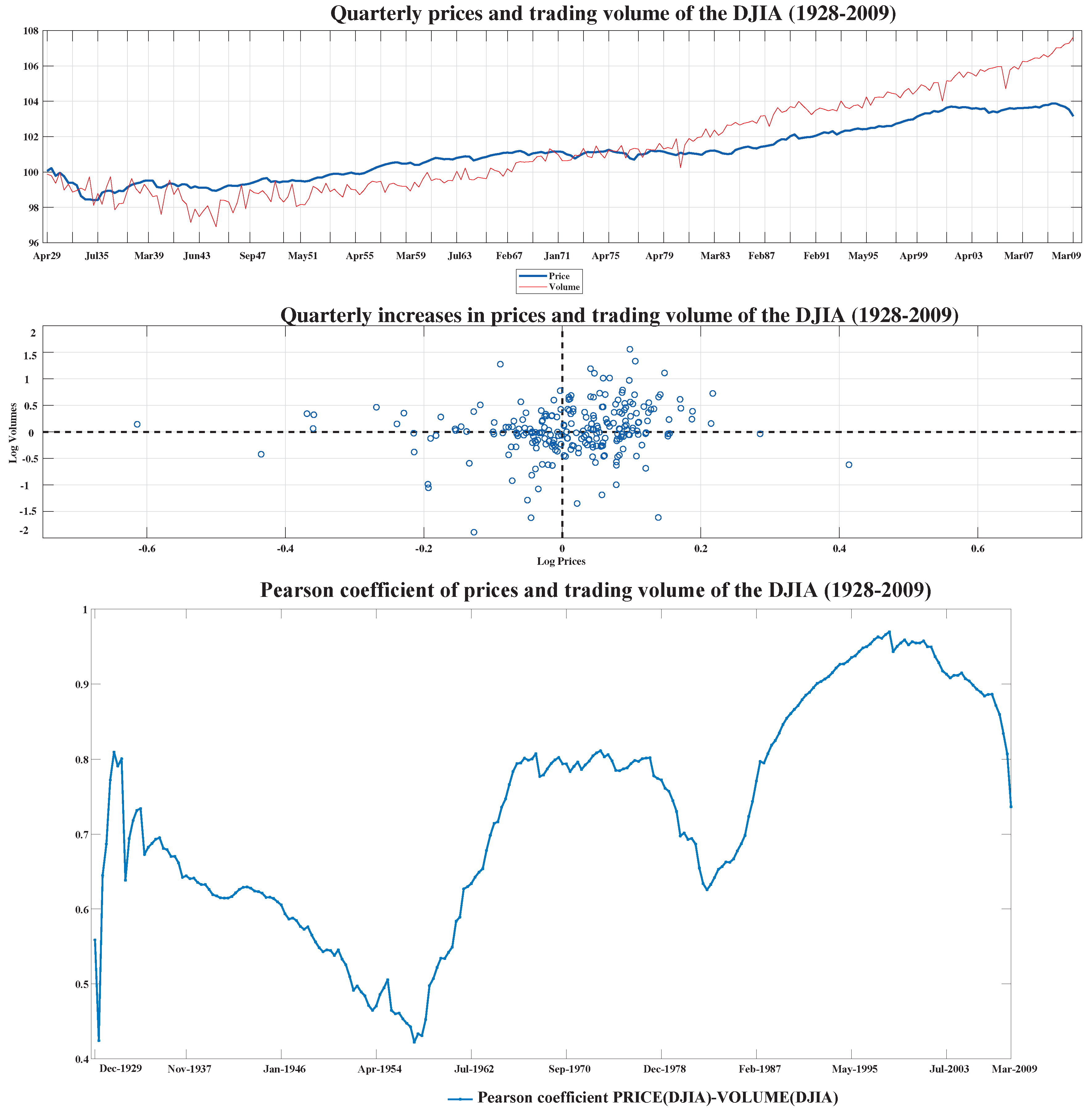
Figure 1 shows the huge level of dispersion and variability of both variables. The first two subfigures, elaborated according to Patton [29], exhibit a normalized time series plot of price (DJIA)–volume (DJIA) as well as a scatter plot of log-increments, both series normalized in base 100, according to the equality $100\times exp\left\{{\sum }_{i=1}^n\frac{ln{X}_i}{ln{X}_{i-1}}\right\}$. The third subfigure represents the Pearson regression coefficient of per se prices and volumes of the DJIA over the analyzed time horizon, showing a quasicyclical relationship between prices and transactional volume within this index, which a priori do not appear to be connected with the evolution of the economic cycle. Several phases or trends can be distinguished: relative decline (1934–1957, 1979–1984, and 2000 onwards), stabilization (1967–1977), and increase (1929–1933, 1958–1966, and 1985–1999) in the relationship between the variables in terms of Pearson’s linear correlation coefficient ($\rho$).

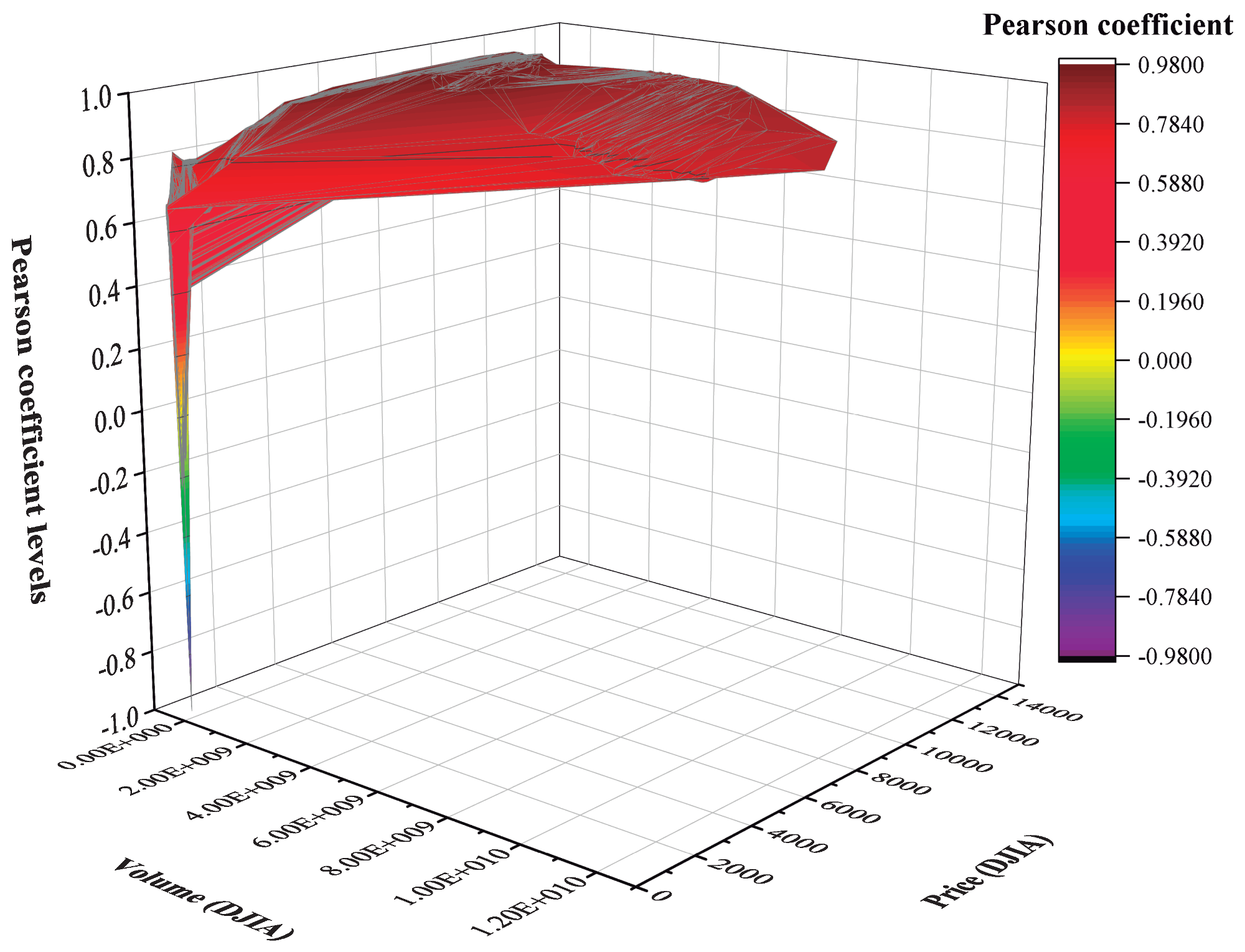
Considering per se magnitudes, Figure 2 presents a three-dimensional scatter plot of the DJIA index that links variables X (volume) and Y (price) to the Pearson linear correlation coefficient (Z = $\rho$). Simply, it can be observed that this chart mostly associates the highest correlation levels of P and V to high per se values of P. Low trading volume per se usually fluctuates within a range from 5.00 × 10${}^9$ to 15.00 × 10${}^9$, although sometimes a relatively high degree of correlation between price and low trading volume can be detected (close to 5.00 × 10${}^9$).

The aim of this paper is to highlight the key aspects of the SRA as an optimal methodological approach for the analysis of the PVR from an empirical perspective that is completely different from the rest of the predominant lines of research. In summary, this methodology can be characterized by: (1) the use of a high number of bivariate copulas (26, see

Table 2. Families of copulas used in this analysis, specifying their corresponding most common mathematical specifications.

Denomination	Mathematical Representation A	Parametric Range	Reference
Gaussian	${\displaystyle {\int }_{-\infty }^{{\varphi }^{-1}\left(u\right)}{\int }_{-\infty }^{{\varphi }^{-1}\left(v\right)}{\displaystyle \frac{1}{2\pi \sqrt{1-{\theta }^2}}}exp\left({\displaystyle \frac{2\theta xy-x^2-y^2}{2(1-{\theta }^2)}}\right)dxdy\mathit{B}}$	$\theta \in [-1,1]$	[102]
t	${\displaystyle {\int }_{-\infty }^{t_{{\theta }_2}^{-1}\left(u\right)}{\int }_{-\infty }^{t_{{\theta }_2}^{-1}\left(v\right)}{\displaystyle \frac{\mathsf{\Gamma }\left(\frac{{\theta }_2+2}{2}\right)}{\mathsf{\Gamma }\left(\frac{{\theta }_2}{2}\right)\pi {\theta }_2\sqrt{1-{\theta }_1^2}}}{\left(1+{\displaystyle \frac{x^2-2{\theta }_{1}xy+{\gamma }^2}{{\theta }_2}}\right)}^{\left(\frac{{\theta }_2+2}{2}\right)}dxdy\mathit{C}}$	${\theta }_1\in [-1,1]\mathrm{and}{\theta }_2\in (0,\infty )$	[102]
Clayton	${\displaystyle max{(u^{-\theta }+y^{-\theta }-1,0)}^{-\frac{1}{\theta }}}$	$\theta \in [-1,\infty )\setminus 0$	[103]
Frank	$-{\displaystyle \frac{1}{\theta }}ln\left[1+{\displaystyle \frac{(exp(-\theta u)-1)(exp(-\theta v)-1)}{exp(-\theta )-1}}\right]$	$\theta \in \mathbb{R}\setminus 0$	[102]
Gumbel	$exp\{-{[{(-ln\left(u\right))}^{\theta }+{(-ln\left(v\right))}^{\theta }]}^{\frac{1}{\theta }}\}$	$\theta \in [1,\infty )$	[102]
Independence	$uv$		[104]
Ali-Mikhail-Haq (AMH)	${\displaystyle {\displaystyle \frac{uv}{1-\theta (1-u)(1-v)}}}$	$\theta \in [-1,1)$	[105]
Joe	$1-{[{(1-u)}^{\theta }+{(1-v)}^{\theta }-{(1-u)}^{\theta }{(1-v)}^{\theta }]}^{\frac{1}{\theta }}$	$\theta \in [1,\infty )$	[102]
Farlie-Gumbel-Morgenstern (FGM)	$uv+\left[\theta \right(1-u\left)\right(1-v\left)\right]$	$\theta \in [-1,1]$	[18]
Gumbel-Barnett	$u+v-1+(1-u)(1-v)exp[-\theta ln(1-u)ln(1-v\left)\right]$	$\theta \in [0,1]$	[55,106]
Plackett	${\displaystyle \frac{1+(\theta -1)(u+v)-\sqrt{{[1+(\theta -1)(u+v)]}^2-4\theta (\theta -1)uv}}{2(\theta -1)}}$	$\theta \in (0,\infty )$	[107]
Cuadras-Auge	${[min(u,v)]}^{\theta }{\left(uv\right)}^{(1-\theta )}$	$\theta \in [0,1]$	[108]
Raftery	$$\left\{\begin{array}{cc}{\displaystyle u-{\displaystyle \frac{1-\theta }{1+\theta }}{u}^{\frac{1}{1-\theta }}(v^{\frac{-\theta }{1-\theta }}-v^{\frac{1}{1-\theta }})}\hfill & \mathrm{if}u\le v\hfill \\ {\displaystyle v-{\displaystyle \frac{1-\theta }{1+\theta }}{v}^{\frac{1}{1-\theta }}(u^{\frac{-\theta }{1-\theta }}-u^{\frac{1}{1-\theta }})}\hfill & \mathrm{if}v\le u\hfill \end{array}\right.$$	$\theta \in [0,1)$	[18]
Shih-Louis	$$\left\{\begin{array}{c}{\displaystyle (1-\theta )uv+\theta min(u,v),\mathrm{if}\theta \in (\theta ,\infty )}\hfill \\ (1+\theta )uv+\theta (u+v^{-1})\mathsf{\Psi }(u+v^{-1}),\mathrm{if}\theta \in (-\infty ,\theta ]\hfill \\ \mathsf{\Psi }\left(a\right)=1,\mathrm{if}a\ge 0\hfill \\ \mathsf{\Psi }\left(a\right)=0,\mathrm{if}a<0\hfill \end{array}\right.$$		[109]
Linear-Spearman	$$\left\{\begin{array}{c}{\displaystyle \left(\right[u+\theta (1-u)]v,\mathrm{if}v\le u\mathrm{and}\theta \in [0,1]}\hfill \\ [v+\theta (1-v\left)\right]u,\mathrm{if}u<v\mathrm{and}\theta \in [0,1]\hfill \\ (1+\theta )uv,\mathrm{if}(u+v)<1\mathrm{and}\theta \in [-1,0]\hfill \\ (uv+\theta (1-u\left)\right(1-v),\mathrm{if}(u+v)\ge 1\mathrm{and}\theta \in [-1,0]\hfill \end{array}\right.$$	$\theta \in [-1,1]$	[110]
Cubic	$uv[1+\theta (u-1\left)\right(v-1\left)\right(2u-1\left)\right(2v-1\left)\right]$	$\theta \in [-1,2]$	[111]
Burr	$u+v-1+{[{(1-u)}^{-\frac{1}{\theta }}+{(1-v)}^{-\frac{1}{\theta }}-1]}^{-\theta }$	$\theta \in (0,\infty )$	[50]
Nelse n	$-{\displaystyle \frac{1}{\theta }}log\left\{1+{\displaystyle \frac{[exp(-\theta u)-1][exp(-\theta v)-1]}{exp(-\theta )-1}}\right\}$	$\theta \in (0,\infty )$	[18]
Galambos	$uvexp{\{{(-ln\left(u\right))}^{-\theta }+{(-ln\left(v\right))}^{-\theta }\}}^{-\frac{1}{\theta }}$	$\theta \in (0,\infty )$	[12]
Marshall-Olkin	$min[u^{(1-{\theta }_1)}v,u{v}^{(1-{\theta }_2)}]$	${\theta }_1,{\theta }_2\in (0,\infty )$	[12]
Fischer-Hinzmann	${\{{\theta }_1{[min(u,v)]}^{{\theta }_2}+(1-{\theta }_1){\left[uv\right]}^{{\theta }_2}\}}^{\frac{1}{{\theta }_2}}$	${\theta }_1\in [0,1],{\theta }_2\in \mathbb{R}$	[112]
Roch-Alegre	$exp\{1-{[{({({(1-ln\left(u\right))}^{{\theta }_1}-1)}^{{\theta }_2}+{({(1-ln\left(v\right))}^{{\theta }_1}-1)}^{{\theta }_2})}^{\frac{1}{{\theta }_2}}+1]}^{\frac{1}{{\theta }_1}}\}$	${\theta }_1\in (0,\infty )$, ${\theta }_2\in [1,\infty )$	[113]
Fischer-Kock	$uv{[1+{\theta }_2(1-u^{\frac{1}{{\theta }_1}})(1-v^{\frac{1}{{\theta }_2}})]}^{{\theta }_1}$	${\theta }_1\in [1,\infty )$, ${\theta }_2\in [-1,1]$
BB1	${\{1+{[{(u^{-{\theta }_1}-1)}^{{\theta }_2}+{(v^{-{\theta }_1}-1)}^{{\theta }_2}]}^{\frac{1}{{\theta }_2}}\}}^{-\frac{1}{{\theta }_1}}$	${\theta }_1\in (0,\infty )$, ${\theta }_2\in (1,\infty )$	[4]
BB5	$exp\{-{[{(-ln\left(u\right))}^{{\theta }_1}+{(-ln\left(v\right))}^{{\theta }_1}-{({(-ln\left(u\right))}^{-{\theta }_1{\theta }_2}+{(-ln\left(v\right))}^{-{\theta }_1{\theta }_2})}^{-\frac{1}{{\theta }_2}}]}^{\frac{1}{{\theta }_1}}\}$	${\theta }_1\in [1,\infty )$, ${\theta }_2\in (0,\infty )$	[4]
Tawn	$exp\{ln\left(u^{(1-{\theta }_1)}\right)+ln\left(v^{(1-{\theta }_2)}\right)-{[{(-{\theta }_{1}ln\left(u\right))}^{{\theta }_3}+{(-{\theta }_{2}ln\left(v\right))}^{{\theta }_3}]}^{\frac{1}{{\theta }_3}}\}$	${\theta }_1,{\theta }_2\in [0$,1], ${\theta }_3\in$[1,∞)	[12]

A. The different formulations of this table do not necessarily have to be unique. B. $\varphi$ represents the distribution Gaussian or standard normal. C. $t_{\theta 2}$ denotes the t student distribution with ${\theta }_2$ degrees of freedom. Source: Specifically readapted to this study from [8].

), especially recommended to simultaneously represent different dependence structures and to conduct prospective inferences based on the chosen variables (not necessarily related to hydrology), such as the variables price and trading volume of a given financial asset or stock index. Notably, to the best of our knowledge, the large number of copulas jointly implemented in the SRA was employed for the first time in the investigation of the PVR. (2) This methodology is based on a unitary reference framework (Bayesian analysis, see Appendix A) in which the hybrid evolution algorithm of the Monte Carlo Markov Chain simulation (MCMCS) was introduced, focusing on the numerical estimation of the subsequent distribution of copula parameters within a context of uncertainty that is relatively similar to the uncertainty observable in financial markets, especially when the different volatility ranges can be conveniently delimited.

As stated by Johannes and Polson [114], the key aspect of the MCMCS is its ability to easily characterize the complete conditional distributions, $p\left(\theta \right|X,Y)$ and $p\left(X\right|\theta ,Y)$, instead of analyzing the higher-dimensional joint distribution $p(\theta ,X|Y)$. The SRA belongs to the class of econometric methods usually applied to the sampling of high-dimensional complex distributions, which implement a hybrid-evolution MCMCS algorithm to infer posterior parameter regions within a Bayesian context. This algorithm is considered a hybrid since it includes a combination of Gibbs steps and Metropolis–Hastings steps [114].

The hybrid-evolution MCMCS algorithm starts with an intelligent starting point selection, structured according to the use of adaptive metropolis (AM), differential evolution (DE), and snooker update.

Table 3. Description of the basis scheme of the hybrid MCMCS algorithm implemented in the SRA approach.

Intelligent prior sampling.

Draw $LN(\ge N)$ samples from prior $\left(p\right(\theta \left)\right)$ using Latin Hypercube Sampling (LHS).

Randomly assign the LHS samples to N complexes.

Selecting the best sample in each complex as the starting point of a Markov chain $\left(\mathit{CH}\right)$.

Snooker update (with a 10% of probability).

Drawing 3 samples, $r_{1-3}$, from parameter space {1 : $D\}\setminus \{i\}$.

Finding the update direction $Z={CH}_j-{CH}_{r_1}$.

Projecting ${CH}_{r2}$ and $\mathrm{C}{H}_{r_3}$ onto Z, to get $Z_{p_1}$ and $Z_{p_2}$.

Creating a proposal ${CH}^{\ast }={CH}_j+{\gamma }_1(Z_{p_2}-Z_{p_1})$.

Computing the Metropolis ratio (1)   ${\displaystyle MR=\frac{\mathcal{L}\left({CH}^{\ast }\right)\left|\right|{CH}^{\ast }-{CH}_{r_1}{\left|\right|}^{D-1}}{\mathcal{L}\left({CH}_i\right)\left|\right|{CH}_i-{CH}_{r_1}{\left|\right|}^{D-1}}}$.

Adaptive Metropolis and differential evolution updating (with a 90% of probability).

Randomly select d dimensions from D-dimensional parameter space to update (within Gibbs sampling).

Creating a proposal sample (1)   ${CH}^{\ast }\left(d\right)={CH}_i\left(d\right)+(1-\beta )N(0_d,{\gamma }_2^2{\mathsf{\Sigma }}_d)+\beta N(0_d,{\gamma }_3^2{I}_d)$.

Creating a proposal sample (2)   ${\displaystyle {CH}^{\ast }\left(d\right)={CH}_i\left(d\right)+{\gamma }_4({CH}_{r_2}\left(d\right)-{CH}_{r_1}\left(d\right))+e}$.

Computing the Metropolis ratio (2)  ${\displaystyle MR=\frac{\mathcal{L}{CH}^{\ast }}{\mathcal{L}{CH}_i}}$.

Accepting proposal $CH$ , with probability $max(MR,1)$, and update current chain, ${CH}_i$.

Checking for Gelman-Rubin $\widehat{R}$ convergence diagnostic.

$LN$ = number of samples drawn from the prior distribution $\left[p\right(\theta \left)\right]$, using Latin Hypercube Sampling (LHS) and N = number of Markov chains ($CH$). D = the dimension of the entire parameter space, d = the dimension of the subspace of the parameters randomly selected for update (Metropolis within Gibbs sampling), T = the total number of iterations, and $N_{AM}$ = the number of chains selected for the Adaptive Metropolis algorithm. ${\gamma }_1-{\gamma }_4$ = “jump factors”, where ${\gamma }_1$ is randomly selected, ${\gamma }_2=2.38/\sqrt{d},{\gamma }_3=0.1/\sqrt{d}$ and ${\gamma }_4=2.38/\sqrt{2d}$. ${\mathsf{\Sigma }}_d$ = adaptive covariance matrix, based on the last 50% samples of the Markov chains. Source: Specifically readapted to this study from [8].

summarizes, in descending order, the working schema implemented in the algorithm developed by Sadegh et al. [8]. For the sake of brevity, intermediate iterative conditions (i.e., end do, end if, etc.) have been omitted from the table.

4. Results

Despite the SRA employing a good number of new generation copulas, with some of them complex in mathematical terms (i.e., Plackett or Shih-Louis),

Table 4. Selection of copulas fitted to the DJIA index (1928–2009) based on three different criteria. Performance-criterion ranking amongst the implemented copulas.

Rank	Max-Likelihood	AIC	BIC	Criteria Coincidence
1	Joe	Joe	Joe	YES
2	Burr	Burr	Burr	YES
3	Fischer-Hinzmann	Fischer-Hinzmann	Fischer-Hinzmann	YES
4	Roch-Alegre	Roch-Alegre	Roch-Alegre	YES
5	Tawn	Tawn	Tawn	YES
6	Gumbel	Gumbel	Gumbel	YES
7	BB5	Galambos	Galambos	NO
8	BB1	BB5	BB5	NO
9	Galambos	BB1	BB1	NO
10	Marshal-Olkin	Marshal-Olkin	Marshal-Olkin	YES
11	Cuadras-Auge	Cuadras-Auge	Cuadras-Auge	YES
12	Nelsen	Nelsen	Nelsen	YES
13	Frank	Frank	Frank	YES
14	Linear-Spearman	Linear-Spearman	Linear-Spearman	YES
15	Shih-Louis	Shih-Louis	Shih-Louis	YES
16	$\mathit{t}$	t	t	YES
17	Gaussian	Gaussian	Gaussian	YES
18	Raftery	Raftery	Raftery	YES
19	Clayton	Clayton	Clayton	YES
20	Plackett	Plackett	Plackett	YES
21	AMH	AMH	AMH	YES
22	FGM	FGM	FGM	YES
23	Fischer-Kock	Fischer-Kock	Fischer-Kock	YES
24	Cubic	Cubic	Cubic	YES
25	Independence	Independence	Independence	YES
26	Gumbel-Barnet	Gumbel-Barnet	Gumbel-Barnet	YES

Souce: Own elaboration.

shows that two copulas with a not very analytically complex, Li et al. [102] and Frees and Valdez [50] best fit the price–volume time series of the DJIA during the considered period (1928–2009), emphasizing that, in all cases, the specified selection criteria coincide except for three copulas: Galambos, BB1, and BB5.

Complementarily,

Table 5. Copula parameters estimation: DJIA (1928–2009).

Copula Name	Rank	RMSE A	NSE B	Par#1-Local	Par#2-Local	Par#3-Local	Par#1-MCMC	95%-Par#1-Unc-Range	Par#2-MCMC	95%-Par#2-Unc-Range	Par#3-MCMC	95%-Par#3-Unc-Range
AMH	21	1.4462	0.9051	1.0000	NaN	NaN	1.0000	[0.9793;0.9998]	NaN	[NaN;NaN]	NaN	[NaN;NaN]
BB1	8	0.1864	0.9984	0.0001	6.8711	NaN	0.0012	[0.0007;0.0890]	6.8738	[6.3355;7.4168]	NaN	[NaN;NaN]
BB5	7	0.1864	0.9984	1.0075	6.1177	NaN	6.8666	[1.0085;7.2476]	0.0434	[0.0260;6.3875]	NaN	[NaN;NaN]
Burr	2	0.1564	0.9989	0.0884	NaN	NaN	0.0884	[0.0832;0.0948]	NaN	[NaN;NaN]	NaN	[NaN;NaN]
Clayton	19	0.2617	0.9969	2.6215	NaN	NaN	27.7501	[22.3225;34.3061]	NaN	[NaN;NaN]	NaN	[NaN;NaN]
Cuadras-Auge	11	0.1919	0.9983	0.9401	NaN	NaN	0.9401	[0.9327;0.9474]	NaN	[NaN;NaN]	NaN	[NaN;NaN]
Cubic	24	2.1634	0.7877	2.0000	NaN	NaN	1.9998	[1.3902;1.9954]	NaN	[NaN;NaN]	NaN	[NaN;NaN]
FGM	22	1.6844	0.8713	1.0000	NaN	NaN	1.0000	[0.9550;0.9999]	NaN	[NaN;NaN]	NaN	[NaN;NaN]
Fischer-Hinzmann	3	0.1653	0.9988	0.9745	−1.7302	NaN	0.9738	[0.9622;0.9814]	−1.7073	[−2.0944;−1.2435]	NaN	[NaN;NaN]
Fischer-Kock	23	1.6846	0.8713	1.0000	1.0000	NaN	1.0005	[1.0015;1.1530]	0.9996	[0.9498;0.9996]	NaN	[NaN;NaN]
Frank	13	0.2041	0.9981	20.1073	NaN	NaN	25.7416	[23.5320;28.7390]	NaN	[NaN;NaN]	NaN	[NaN;NaN]
Galambos	9	0.1865	0.9984	6.1687	NaN	NaN	6.1688	[5.6654;6.7940]	NaN	[NaN;NaN]	NaN	[NaN;NaN]
Gaussian	17	0.2131	0.9979	0.9140	NaN	NaN	0.9785	[0.9735;0.9827]	NaN	[NaN;NaN]	NaN	[NaN;NaN]
Gumbel	6	0.1864	0.9984	4.3567	NaN	NaN	6.8717	[6.3810;7.5823]	NaN	[NaN;NaN]	NaN	[NaN;NaN]
Gumbel-Barnet	26	2.2788	0.7645	0.0000	NaN	NaN	0.0000	[0.0003;0.0321]	NaN	[NaN;NaN]	NaN	[NaN;NaN]
Independence	25	2.2788	0.7645	NaN	NaN	NaN	NaN	[NaN;NaN]	NaN	[NaN;NaN]	NaN	[NaN;NaN]
Joe	1	0.1563	0.9989	12.0596	NaN	NaN	12.0583	[11.3142;12.9402]	NaN	[NaN;NaN]	NaN	[NaN;NaN]
Linear-Spearman	14	0.2079	0.9980	0.9238	NaN	NaN	0.9238	[0.9113;0.9340]	NaN	[NaN;NaN]	NaN	[NaN;NaN]
Marshal-Olkin	10	0.1893	0.9984	8.6736	0.1012	NaN	0.9484	[0.9382;0.9714]	0.9298	[0.9019;0.9410]	NaN	[NaN;NaN]
Nelsen	12	0.2041	0.9981	24.0724	NaN	NaN	25.7465	[23.6645;28.8592]	NaN	[NaN;NaN]	NaN	[NaN;NaN]
Plackett	20	0.4651	0.9902	35.0000	NaN	NaN	34.9994	[34.0284;34.9944]	NaN	[NaN;NaN]	NaN	[NaN;NaN]
Raftery	18	0.2602	0.9969	0.9522	NaN	NaN	0.9522	[0.6394;0.9791]	NaN	[NaN;NaN]	NaN	[NaN;NaN]
Roch-Alegre	4	0.1707	0.9987	0.0001	9.0334	NaN	0.0007	[0.0029;0.1435]	9.0521	[8.3601;9.7642]	NaN	[NaN;NaN]
Shih-Louis	15	0.2079	0.9980	0.9238	NaN	NaN	0.9237	[0.9128;0.9348]	NaN	[NaN;NaN]	NaN	[NaN;NaN]
t	16	0.2085	0.9980	0.9363	3.9764	NaN	0.9809	[0.9745;0.9849]	0.5611	[0.2827;30.9390]	NaN	[NaN;NaN]
Tawn	5	0.1793	0.9985	0.9787	0.9466	11.5247	0.9786	[0.9580;0.9957]	0.9457	[0.9233;0.9662]	11.6332	[8.4142;23.0476]

A. Root Mean Square Error. B. Nash-Sutcliff Efficiency. Source: Own elaboration.

provides estimations of the parameters of each copula (Par) by fixing a range of 95% of uncertainty in their estimation (Unc-Range) through the application of local optimization and MCMCS. The copulas with best performance (Rank) are defined in terms of the root mean square error (RMSE) and the Nash–Sutcliff Efficiency (NSE) criteria. At this point, the existing literature usually employs local optimization algorithms when estimating the parameters of copulas with the consequent risk of being trapped in local optima, thus often obtaining unbiased and nonsignificant results [8]. Conversely, the hybrid-evolution MCMCS algorithm used in the SRA overcomes this initial limitation by determining an efficient estimator of the global optimum as well as an accurate approximation of uncertainties in the content of a Bayesian conceptual framework in the form of isolines, which is another of the improvements provided by this methodology to PVR analysis.

The analysis of the SRA applied to the NIKKEI225, FTSE100, and IBEX35 indices using the Tawn’s copula is summarized in

Table 6. Tawn copula parameters estimation: NIKKEI225, IBEX35, and FTSE100 (2000–2018).

Index	RMSE	NSE	Par#1-Local	Par#2-Local	Par#3-Local	Par#1-MCMC	95%-Par#1-Unc-Range	Par#2-MCMC	95%-Par#2-Unc-Range	Par#3-MCMC	95%-Par#3-Unc-Range
NIKKEI 225	0.2621	0.9914	0.0744	0.2153	34.9816	0.0738	[0.0551–0.1248]	0.219	[0.0977–0.4725]	25.9197	[2.2342–34.4984]
IBEX 35	0.3901	0.9737	0.005	0.8691	11.1339	0.0049	[0.0000–0.9876]	0.9969	[0.0000–0.9969]	22.6851	[1.0000–34.4965]
FTSE 100	0.9005	0.8235	0.3857	0	13.1732	0.0097	[0.0000–0.9896]	0.5024	[0.0000–0.9881]	1	[1.0000–35.0000]

Source: Own elaboration.

, similarly to Table 5. The price–volume dependence structure of the per se NIKKEI225 index is optimal in accordance with the NSE criterion, as it is very close to unity (0.9914), indicating an almost perfect model fitting. The per se IBEX35 adjustment is relatively optimal (0.9737), being lower for the FTSE100 (0.8235). The range of uncertainty of the parameters defining the Tawn’s copula (${\theta }_1$, ${\theta }_2$, and ${\theta }_3$, Table 2) is considerably lower in the Nippon index than in the other two stock market indices.

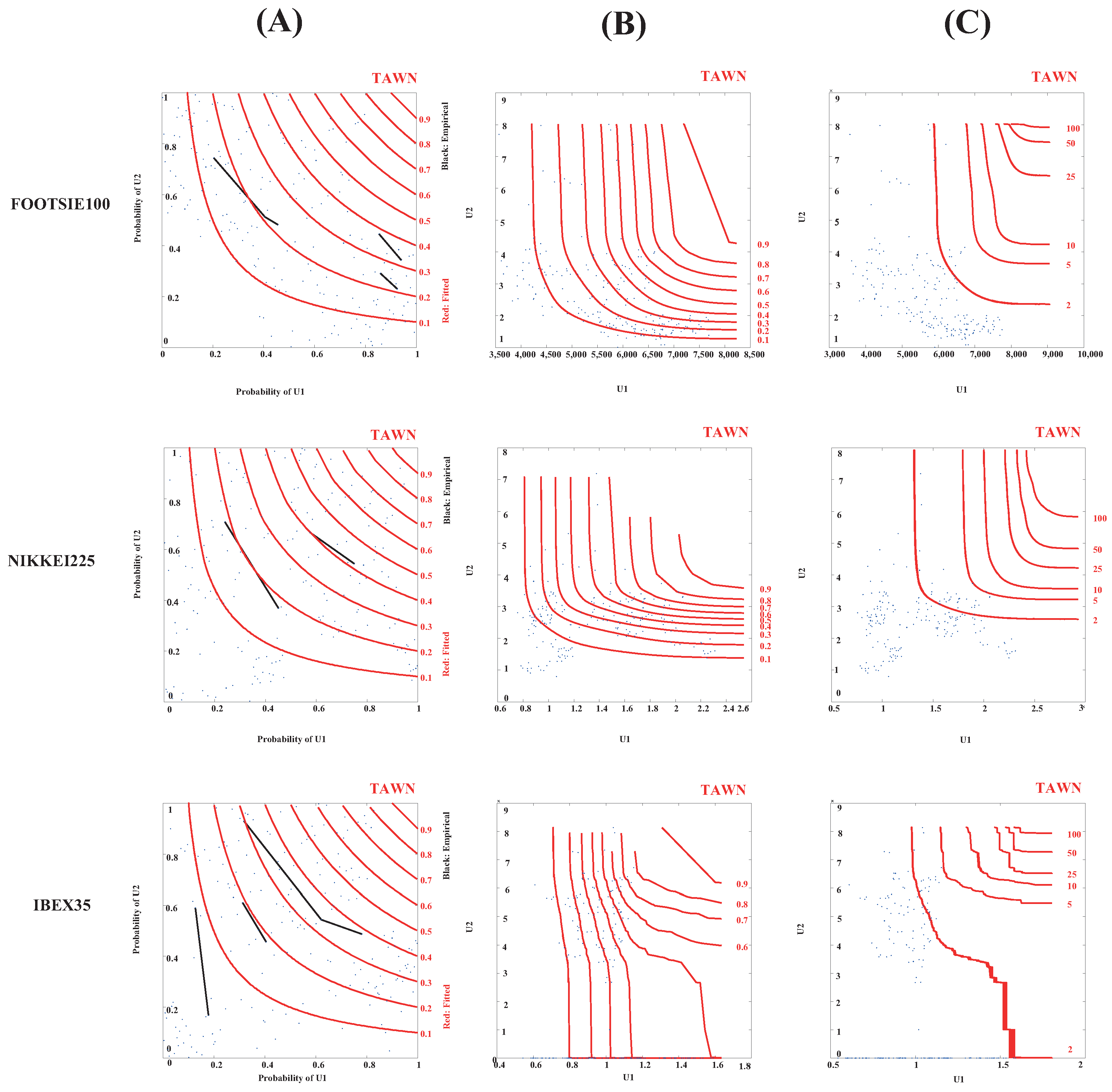
Figure 3 shows that each stock exchange index corresponds to a certain typology of its probability isolines. Rows 1 to 3 refer to the analyzed indices, whereas columns correspond to the following specifications: (A) fitted empirical copulas probabilities, (B) fitted empirical copulas, and (C) return period copulas, calculated according to [115] by considering the joint return $\left(\frac{1}{1-C(u,v)}\right)$ as a measure of the dependence structure between the observed price peaks and trading volumes.

The isolines derived from the application of Tawn’s copula are ostensibly biased toward the upper left corner, which seems to indicate a low probability of occurrence of the price ($U_1$) synchronously linked to a high probability of occurrence of the trading volume ($U_2$) (both measured in magnitudes per se). Likewise, given the joint representation of the probability isolines and the empirical estimates of the joint probability distributions, the trends of the FOOTSIE100 and NIKKEI225 indices are fairly similar, although in the former index, high prices use to be related to trading volumes lower than those shown in the Japanese stock market. The P—V relationship in the IBEX35, although following a similar pattern, differs to some extent from the analysis of the other two indices, as low prices seem to be more related to high trading volumes quotas. This type of asymmetric and skewed dependence structure can be considered a common pattern of the three indices analyzed, equally extrapolated to the analysis of the fitted empirical copulas and return period copulas.

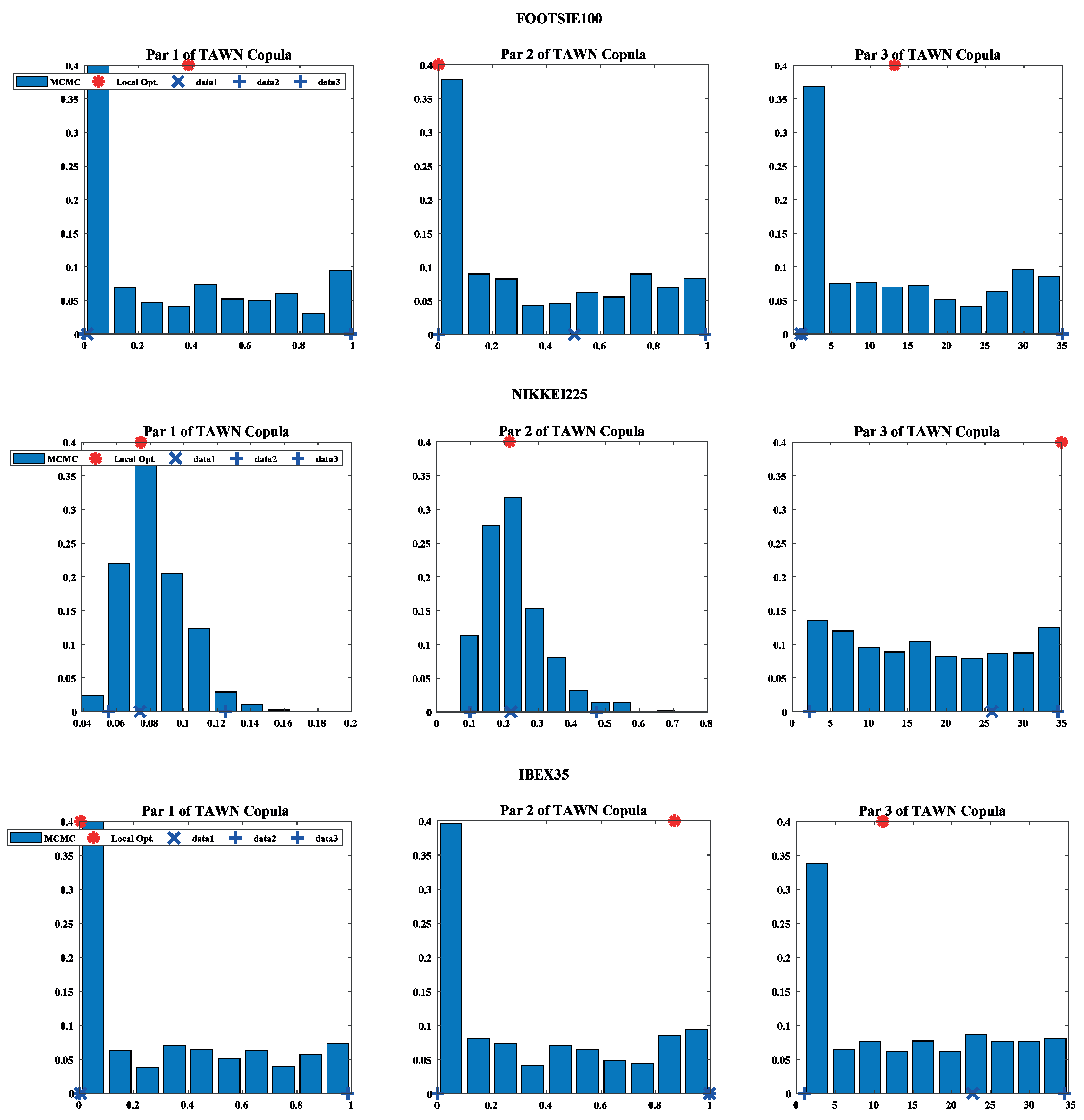
Figure 4 shows the degree of uncertainty associated with the three parameters defining the Tawn’s copula. Figure 4 exhibits the specification of the copula parameters generated by the MCMCS through a Bayesian framework. Blue bins represent the MCMC-obtained parameters, blue crosses (bottom of each plot) denote the maximum likelihood estimation parameters, and red asterisks (top of each plot) indicate the copula parameter value obtained by local optimization.

In a context characterized by minimal uncertainty when specifying the parameters of the copula in each market, the parameters obtained by the local optimization algorithm should coincide with the mode of the distribution calculated through the MCMCS. However, this was only observed in the NIKKEI225 (parameters 1 and 2) and IBEX35 (parameter 1) and was not contrastable for any of the three parameters obtained from the Tawn’s copula to the FOOTSIE100 index. These results are consistent with the previously calculated uncertainty ranges and with the delimitation of the degree of goodness of the adjustment performed by the NSE criteria (Table 6), according to which the NIKKEI225 index represented a quasiperfect fitting to this copula, followed by the IBEX35, and, to a lesser extent, the FOOTSIE100. This can be justified by the different range of variation of the parameters obtained for each index, where the FOOTSIE100 index is associated with a higher level of uncertainty compared with NIKKEI225 and IBEX35.

5. Discussion

The application of the SRA provides an alternative and innovative approach to PVR based on the simultaneous application of 26 copulas, which facilitated the analysis of their dependence structures and implicit morphology according with their probability isolines. Many of these copulas are dissimilar in form, although quite similar in performance. This also allowed us to model the relationship between prices and trading volumes from different points of view, quantifying the uncertainty underlying to the specification of the parameters defining each copula. The PVR, usually characterized by a markedly asymmetric relationship [13], is reinforced by the application of the SRA, since several of the copulas used in this methodology (e.g., Galambos, Bernstein, Tawn, etheory of copulas.) are especially effective in the study of phenomena with underlaying asymmetric skewed dependence structures.

From an empirical point of view, the joint implementation of the 26 copulas in the DJIA (generic scenario) confirmed that Joe’s copula is able to more efficiently model the dependence structures of this index. Framing our findings with the existing literature, the use of Tawn’s copula in the FOOTSIE100, NIKKEI225, and IBEX35 indices (specific scenario) confirms Ying [68]’s findings in their seminal analysis of the S&P 500 index. Similarly, our results confirm the analysis of the NIKKEI225 completed by Bremer and Kato [116], according to which an asymmetric relationship could be observed (negative correlation between past prices and current trading volume). This relationship was explained in the FOOTSIE100 by Huang and Masulis [117] based on the existence of a minority of informed-trading investors who simply sought immediate liquidity. The asymmetric PVR detected in the IBEX35 aligns with that already reported in the literature (see, for example, [118]). Its differentiated nature with respect to the other two indices is probably due to, according to [119] in the Spanish financial markets (Mercado Continuo), a strong linear causal relationship from returns to trading volume. Specifically, periods with high returns are usually followed by periods with particularly high trading volume. Such guidelines are comparable to those detected in other works [95,97], which explicitly used copulas in the study of PVR in the Asian financial markets, repeatedly verifying the existence of an inverse relationship between prices and volumes traded, in both cases foreseeably increased by the effects of the 1997 Asian financial crisis.

One of the improvements associated with the application of the SAR approach to the PVR is facilitating the analysis of both variables from a large number of copulas by defining the relationship based on ranges of uncertainty applying the RMSE and NSE criteria (see Table 5 and Table 6), independent of the degree or sign of the linear correlation exhibited by the Pearson correlation coefficient ($\rho$), which, to the best of our knowledge, is an entirely new application in the field of quantitative finance of future utility for researchers and investors.

6. Conclusions

The main contribution of this research is the analysis of the existing relationship between prices and trading volume from multiple copulas, which allowed us to comparatively abstract the underlying dependency structures of both variables to establish possible analogies or differences. One of the most important limitations related to the empirical application of copulas is solved, which is employing a limited number of standard copulas when, in reality, there are multiple copulas not yet well extended in the literature [11]. Through the empirical methodology introduced in this article, the versatility of copulas increases when they are simultaneously combined with the polyvalence of the Bayesian analysis and with the hybrid-evolution MCMCS algorithm proposed by Sadegh et al. [8]. We are the first to implement the SRA, not just in PVR analysis, but in the ambit of quantitative finance. More specifically, for practical purposes, PVR analysis is decisive for both academics and practitioners, since, following the scheme constructed by Karpoff [13], it has the following implications: (1) it generates additional information regarding the structure of financial markets; (2) from an empirical point of view, it is fundamental in the generation of case studies that jointly use prices and trading volume, facilitating the implementation of analyses and inferences; (3) it is a crucial element in the study of the empirical distribution of speculative prices; and (4) its research would be particularly indicated in the futures markets where, a priori, the variability of prices used to affect the trading volume.

Additionally, we tried to answer and reconcile three questions linked to the theory of copulas: which copula is the “right one” [120], which copula should be used [20], and why copulas have been successful in many practical applications [44]? Versatility is the key term that best defines a copula; therefore, the most appropriate copula for analyzing a particular issue is the one that best summarizes its implicit dependence structures. Hence, copulas have been so successful in different fields of study.

A first conclusion to be drawn from this work is that the potential of the theory of copulas could be significantly reduced if certain copulas-type are systematically used in the analysis of bivariate time series. Precisely, this was the factor that caused a certain reluctance toward the use of copulas when the Gaussian copula [10] was employed massively in almost any scientific field, without considering either the intrinsic nature of the phenomena analyzed or that the use of a large number of copulas can substantially improve the knowledge of the different relations of dependence observable in a given dataset [50]. Thus, the SRA is not simply limited to the task of choosing and fitting the copula [121], but following the transdisciplinary perspective of econophysics, it supposes a new framework in the analysis of the PVR, extrapolated from the field of hydrology, which is directly applicable to many other areas such as quantitative finance.

Since Karpoff [13], the PVR has been practically subsumed to the generalization of the significance of Pearson’s linear correlation coefficient of the price and trading volume variables. However, an alternative is provided in this methodology since the classical optimization methods applied to copulas often get trapped in local minima. The SRA is able to conveniently overcome this limitation by accurately describing the dependence structure of variables P and V and, importantly, by allowing the analysis of uncertainties given a determined time horizon (or length of record, see [8]). Another contribution of this work that may be important for future lines of research is the incorporation in the methodology of copula probability isolines in the analysis of PVR, which approximates this research to the multifractal models of Mandelbrot [22].

In our opinion, other future lines of research related to this work include, for example, the analysis of the role played by floating capital (outstanding shares vs. restricted shares) in the context of PVR, an aspect which has been often overlooked in the literature, or the rigorous enunciation and detailed compilation of those empirical stylized facts defining the price–volume time series, as well as the definitive consolidation of the works that have analyzed PVR from the perspective of the market microstructure of Garman [122]. This research could be gradually applied to the area of behavioral finance following the path of works such as Gomes [123], in which the analysis of PVR is directly connected to the prospective theory of Kahneman and Tversky [124].

References

1. Jovanovic, F.; Schinckus, C. The History of Econophysics’ Emergence: A New Approach in Modern Financial Theory. Hist. Political Econ. 2013, 45, 443–474. [Google Scholar] [CrossRef] [Green Version]
2. Schinckus, C.; Jovanovic, F. Towards a transdisciplinary econophysics. J. Econ. Methodol. 2013, 20, 164–183. [Google Scholar] [CrossRef] [Green Version]
3. Hurst, H.E. Long Term Storage Capacity of Reservoirs. Trans. Am. Soc. Civ. Eng. 1951, 116, 770–799. [Google Scholar]
4. Genest, C.; Favre, A.C. Everything You Always Wanted to Know about Copula Modeling but Were Afraid to Ask. J. Hydrol. Eng. 2007, 12, 347–368. [Google Scholar] [CrossRef]
5. Reiß, R.D.; Thomas, M. Statistical Analysis of Extreme Values: With Applications to Insurance, Finance, Hydrology and Other Fields; Birkhäuser: Basel, Switzerland, 2007. [Google Scholar]
6. Schweizer, B. Introduction to Copulas. J. Hydrol. Eng. 2007, 12, 346. [Google Scholar] [CrossRef] [Green Version]
7. Genest, C. Everything You Always Wanted to Know about Copula Modeling but Were Afraid to Ask. In Proceedings of the NIPS 2011 Workshop on Copulas in Machine Learning, Sierra Nevada, Spain, 16 December 2011; Technical Report. American Society of Civil Engineers: Reston, VA, USA, 2011. [Google Scholar]
8. Sadegh, M.; Ragno, E.; AghaKouchak, A. Multivariate Copula Analysis Toolbox (MvCAT): Describing dependence and underlying uncertainty using a Bayesian framework. Water Resour. Res. 2017, 53. [Google Scholar] [CrossRef]
9. Genest, C.; Gendron, M.; Bourdeau-Brien, M. The Advent of Copulas in Finance. Eur. J. Financ. 2009, 15, 609–618. [Google Scholar] [CrossRef]
10. Li, D.X. On Default Correlation: A Copula Function Approach. J. Fixed Income 2000, 9, 4. [Google Scholar] [CrossRef]
11. Nadarajah, S.; Afuecheta, E.; Chan, S. A Compendium of Copulas. In Probability and Statistics Group School of Mathematics, Research Reports; Technical Report 10; The University of Manchester: Manchester, UK, 2016. [Google Scholar]
12. Huynh, V.N.; Inuiguchi, M.; Denoeux, T. (Eds.) Integrated Uncertainty in Knowledge Modelling and Decision Making: Proceedings of the 4th International Symposium, IUKM 2015, Nha Trang, Vietnam, 15–17 October 2015; Lecture Notes in Artificial Intelligence; Springer International Publishing: Cham, Switzerland, 2015; Volume 9376. [Google Scholar]
13. Karpoff, J.M. The Relation between Price Changes and Trading Volume: A Survey. J. Financ. Quant. Anal. 1987, 22, 109–126. [Google Scholar] [CrossRef]
14. Martín Cervantes, P.A. Hacia un Modelo Estocástico Eficiente Para la Valoración de Activos Financieros Basado en el Volumen de Negociación: Fundamentos Teóricos e Implementación Práctica. Ph.D. Thesis, Universidad de Almería, Almería, Spain, 2017. [Google Scholar]
15. Sklar, A. Fonctions de répartition à n dimensions et leurs marges. Publ. L’Institut Stat. L’Université Paris 1959, 8, 229–231. [Google Scholar]
16. Quesada, J.J.; Rodríguez, J.A.; Úbeda, M. What are copulas? In Monografías del Seminario Matemático García de Galdeano; Universidad de Zaragoza: Zaragoza, Spain, 2003; pp. 499–506. [Google Scholar]
17. Joe, H. Multivariate Models and Multivariate Dependence Concepts; Chapman & Hall/CRC Monographs on Statistics & Applied Probability; Springer Science & Business Media: Berlin/Heidelberg, Germany, 1997; Volume 73. [Google Scholar]
18. Nelsen, R.B. An Introduction to Copulas, 1st ed.; Lecture Notes in Statistics; Springer: New York, NY, USA, 1999; Volume 139. [Google Scholar]
19. Durante, F.; Sempi, C. Principles of Copula Theory; CRC Press: Boca Raton, FL, USA, 2015. [Google Scholar]
20. Embrechts, P. Copulas: A Personal View. J. Risk Insur. 2009, 76, 639–650. [Google Scholar] [CrossRef]
21. Daníelsson, J. Financial Risk Forecasting: The Theory and Practice of Forecasting Market Risk with Implementation in R and Matlab; The Wiley Finance Series; John Wiley & Sons: Chichester, UK, 2011. [Google Scholar]
22. Mandelbrot, B.B. Heavy Tails in Finance for Independent or Multifractal Price Increments. In Handbook of Heavy Tailed Distributions in Finance; Rachev, S.T., Ed.; North-Holland: Amsterdam, The Netherlands, 2003; Volume 1, Chapter 1; pp. 1–34. [Google Scholar]
23. Rachev, S.T.; Menn, C.; Fabozzi, F.J. Copulas. In Fat-Tailed & Skewed Asset Return Distributions: Implications for Risk Management, Portfolio Selection, and Option Pricing; Chapter 6; John Wiley & Sons: Hoboken, NJ, USA, 2005; pp. 71–80. [Google Scholar]
24. Junker, M.; Szimayer, A.; Wagner, N. Nonlinear term structure dependence: Copula functions, empirics, and risk implications. J. Bank. Financ. 2006, 30, 1171–1199. [Google Scholar] [CrossRef]
25. Ning, C.; Xu, D.; Wirjanto, T.S. Modeling Asymmetric Volatility Clusters Using Copulas and High Frequency Data; Technical Report 6, Working Papers; Ryerson University, Department of Economics: Toronto, ON, Canada, 2009. [Google Scholar]
26. Ibragimov, R.; Mo, J.; Prokhorov, A. Fat Tails and Copulas: Limits of Diversification Revisited; Technical Report 2015-06, Working Papers; University of Sydney Business School, Discipline of Business Analytics: Sydney, Australia, 2015. [Google Scholar]
27. Patton, A.J. Copula-Based Models for Financial Time Series. In Handbook of Financial Time Series; Andersen, T.G., Davis, R.A., Kreiß, J.P., Mikosch, T.V., Eds.; Mathematics and Statistics; Springer Science & Business Media: Berlin/Heidelberg, Germany, 2009; pp. 767–786. [Google Scholar]
28. Patton, A.J. A review of copula models for economic time series. J. Multivar. Anal. 2012, 110, 4–18. [Google Scholar] [CrossRef] [Green Version]
29. Patton, A.J. Copula Methods for Forecasting Multivariate Time Series. In Handbook of Economic Forecasting; Elliott, G., Timmermann, A., Eds.; Elsevier/North Holland: Amsterdam, The Netherlands, 2013; Volume 2, Chapter 16; pp. 899–960. [Google Scholar]
30. Giacomini, E.; Härdle, W.; Spokoiny, V. Inhomogeneous Dependence Modeling with Time-Varying Copulae. J. Bus. Econ. Stat. 2009, 27, 224–234. [Google Scholar] [CrossRef]
31. Manner, H.; Reznikova, O. A Survey on Time-Varying Copulas: Specification, Simulations, and Application. Econom. Rev. 2012, 31, 654–687. [Google Scholar] [CrossRef]
32. Patton, A.J. Modelling asymmetric exchange rate dependence. Int. Econ. Rev. 2006, 47, 527–556. [Google Scholar] [CrossRef]
33. Patton, A.J. On the out-of-sample importance of skewness and asymmetric dependence for asset allocation. J. Financ. Econom. 2004, 2, 130–168. [Google Scholar] [CrossRef] [Green Version]
34. Embrechts, P.; Höing, A.; Juri, A. Using copulae to bound the Value-at-Risk for functions of dependent risks. Financ. Stochastics 2003, 7, 145–167. [Google Scholar] [CrossRef]
35. Cherubini, U.; Luciano, E. Bivariate option pricing with copulas. Appl. Math. Financ. 2002, 9, 69–85. [Google Scholar] [CrossRef]
36. Van den Goorbergh, R.W.; Genest, C.; Werker, B.J. Bivariate option pricing using dynamic copula models. Insur. Math. Econ. 2005, 37, 101–114. [Google Scholar] [CrossRef]
37. Chiou, S.C.; Tsay, R.S. A copula-based approach to option pricing and risk assessment. J. Data Sci. 2008, 6, 273–301. [Google Scholar]
38. Morillas, P.M. A method to obtain new copulas from a given one. Metrika 2005, 61, 169–184. [Google Scholar] [CrossRef]
39. Chen, X.; Fan, Y. Estimation and model selection of semiparametric copula-based multivariate dynamic models under copula misspecification. J. Econom. 2006, 135, 125–154. [Google Scholar] [CrossRef] [Green Version]
40. García, C.; Herrerías, J.M.; Trinidad, J.E. Making Copulas Under Uncertainty. In Distribution Models Theory; Herrerías, R., Callejón, J., Herrerías, J.M., Eds.; World Scientific Publishing: Singapore, 2006; Chapter 2; pp. 27–53. [Google Scholar]
41. Genest, C.; Remillard, B.; Beaudoin, D. Goodness-of-fit tests for copulas: A review and a power study. Insur. Math. Econ. 2009, 44, 199–213. [Google Scholar] [CrossRef]
42. Joe, H.; Kurowicka, D. Dependence Modeling: Vine Copula Handbook; World Scientific Publishing: Singapore, 2011. [Google Scholar]
43. Kiatmanaroch, T.; Sriboonchitta, S. Relationship between Exchange Rates, Palm Oil Prices, and Crude Oil Prices: A Vine Copula Based GARCH Approach. In Modeling Dependence in Econometrics: Selected Papers of the 7th International Conference of the Thailand Econometric Society, Faculty of Economics, Chiang Mai University, Thailand, 8–10 January 2014; Huynh, V.N., Kreinovich, V., Sriboonchitta, S., Eds.; Advances in Intelligent Systems and Computing; Springer International Publishing: Cham, Switzerland, 2014; Volume 251, pp. 399–413. [Google Scholar]
44. Kreinovich, V.; Nguyen, H.T.; Sriboonchitta, S.; Kosheleva, O. Why Copulas Have Been Successful in Many Practical Applications: A Theoretical Explanation Based on Computational Efficiency. In Integrated Uncertainty in Knowledge Modelling and Decision Making: Proceedings of the 4th International Symposium, IUKM 2015, Nha Trang, Vietnam, 15–17 October 2015; Huynh, V.N., Inuiguchi, M., Denoeux, T., Eds.; Lecture Notes in Artificial Intelligence; Springer International Publishing: Cham, Switzerland, 2015; Volume 9376, pp. 112–126. [Google Scholar]
45. Embrechts, P.; Mcneil, A.J.; Straumann, D. Correlation and dependence in risk management. In Proceedings of the ASTIN Colloquium, Tokyo, Japan, 22–25 August 1999; Cambridge University Press: Cambridge, UK, 1999; pp. 176–223. [Google Scholar]
46. McNeil, A.J.; Frey, R.; Embrechts, P. Quantitative Risk Management: Concepts, Techniques, and Tools: Concepts, Techniques, and Tools; Princeton Series in Finance; Princeton University Press: Princeton, NJ, USA, 2005. [Google Scholar]
47. Schweizer, B.; Sklar, A. Probabilistic Metric Spaces; North Holland Series in Probability and Applied Mathematics; North Holland: Amsterdam, The Netherlands, 1983. [Google Scholar]
48. Genest, C.; Nešlehová, J. A Primer on Copulas for Count Data. Astin Bull. 2007, 37, 475–515. [Google Scholar] [CrossRef] [Green Version]
49. Mayor, G.; Suñer, J.; Torrens, J. Sklar’s Theorem in Finite Settings. IEEE Trans. Fuzzy Syst. 2007, 15, 410–416. [Google Scholar] [CrossRef]
50. Frees, E.; Valdez, E. Understanding Relationships Using Copulas. N. Am. Actuar. J. 1998, 2, 1–25. [Google Scholar] [CrossRef]
51. Bouyé, E.; Durrleman, V.; Nikeghbali, A.; Riboulet, G.; Roncalli, T. Copulas for Finance—A Reading Guide and Some Applications; Technical Report; Crédit Lyonnais, Groupe de Recherche Opérationnelle: Paris, France, 2000. [Google Scholar]
52. Mikosch, T. Copulas: Tales and facts. Extremes 2006, 9, 3–20. [Google Scholar] [CrossRef]
53. Shiller, R.J. Irrational Exuberance; New York Times Bestseller, Broadway Books: New York, NY, USA, 2001. [Google Scholar]
54. Donnelly, C.; Embrechts, P. The Devil is in the Tails: Actuarial Mathematics and the Subprime Mortgage Crisis. Astin Bull. J. Int. Actuar. Assoc. 2010, 40, 1–33. [Google Scholar] [CrossRef] [Green Version]
55. Gumbel, E.J. Bivariate Exponential Distributions. J. Am. Stat. Assoc. 1960, 55, 698–707. [Google Scholar] [CrossRef]
56. Embrechts, P.; Mcneil, A.J.; Straumann, D. Correlation and dependence in risk management: Properties and pitfalls. In RISK Management: Value at Risk and Beyond; Cambridge University Press: Cambridge, UK, 2002; pp. 176–223. [Google Scholar]
57. Schachermayer, W. Mathematics and Finance. In Proceedings of the 7th European Congress of Mathematics (7ECM), Berlin, Germany, 18–22 July 2016. Technical report, The German Mathematical Society (DMV), the International Association of Applied Mathematics and Mechanics (GAMM), the Research Center Matheon, the Einstein Center ECMath and the Berlin Mathematical School (BMS). [Google Scholar]
58. Daníelsson, J. The emperor has no clothes: Limits to risk modelling. J. Bank. Financ. 2002, 26, 1273–1296. [Google Scholar] [CrossRef]
59. Zimmer, D.M. The Role of Copulas in the Housing Crisis. Rev. Econ. Stat. 2012, 94, 607–620. [Google Scholar] [CrossRef]
60. Salmon, F. The formula that killed Wall Street. Significance 2012, 9, 16–20. [Google Scholar] [CrossRef]
61. Rogers, L.C.G. Document in response to questions posed by Lord Drayson, UK Science and Innovation Minister. Financ. Math. Credit. Crisis 2009. [Google Scholar]
62. Osborne, M.F.M. Brownian Motion in the Stock Market. Oper. Res. 1959, 7, 145–173. [Google Scholar] [CrossRef]
63. Samuelson, P.A. Rational Theory of Warrant Pricing. Ind. Manag. Rev. 1965, 6, 13–39. [Google Scholar]
64. Granger, C.W.J.; Morgenstern, O. Spectral analysis of New York stock market prices. Kyklos 1963, 16, 1–27. [Google Scholar] [CrossRef]
65. Godfrey, M.D.; Granger, C.W.J.; Morgenstern, O. The Random Walk Hypothesis of Stock Market Behavior. Kyklos 1964, 17, 1–30. [Google Scholar] [CrossRef]
66. Morgenstern, O. Demand Theory Reconsidered. Q. J. Econ. 1948, 62, 165–201. [Google Scholar] [CrossRef]
67. Granger, C.W.J. Investigating Causal Relations by Econometric Models and Cross-Spectral Methods. Econometrica 1969, 37, 424–438. [Google Scholar] [CrossRef]
68. Ying, C.C. Stock Market Prices and Volumes of Sales. Econometrica 1966, 34, 676–685. [Google Scholar] [CrossRef]
69. Clark, P.K. A Subordinated Stochastic Process Model with Finite Variance for Speculative Prices. Econometrica 1973, 41, 135–155. [Google Scholar] [CrossRef]
70. Epps, T.W. Security Price Changes and Transaction Volumes: Theory and Evidence. Am. Econ. Rev. 1975, 65, 586–597. [Google Scholar]
71. Epps, T.W.; Epps, M.L. The Stochastic Dependence of Security Price Changes and Transaction Volumes: Implications for the Mixture-of-Distributions Hypothesis. Econometrica 1976, 44, 305–321. [Google Scholar] [CrossRef]
72. Tauchen, G.E.; Pitts, M. The Price Variability-Volume Relationship on Speculative Markets. Econometrica 1983, 51, 485–505. [Google Scholar] [CrossRef] [Green Version]
73. Andersen, T.G. Return volatility and trading volume: An information flow interpretation of stochastic volatility. J. Financ. 1996, 51, 169–204. [Google Scholar] [CrossRef]
74. García, J. Volumen y volatilidad en mercados financieros: El caso del mercado de futuros español. Rev. Espa NOla Financ. Contab. 1998, XXVII, 367–393. [Google Scholar]
75. Lamoureux, C.G.; Lastrapes, W.D. Heteroskedasticity in Stock Return Data: Volume versus GARCH Effects. J. Financ. 1990, 45, 221–229. [Google Scholar] [CrossRef]
76. Lamoureux, C.G.; Lastrapes, W.D. Endogenous Trading Volume and Momentum in Stock-Return Volatility. J. Bus. Econ. Stat. 1994, 12, 253–260. [Google Scholar]
77. Bollerslev, T. Generalized Autoregressive Conditional Heteroskedasticity. J. Econom. 1986, 31, 307–327. [Google Scholar] [CrossRef] [Green Version]
78. Copeland, T.E. A Model of Asset Trading under the Assumption of Sequential Information Arrival. J. Financ. 1976, 31, 1149–1168. [Google Scholar] [CrossRef]
79. Copeland, T.E. A Probability Model of Asset Trading. J. Financ. Quant. Anal. 1977, 12, 563–578. [Google Scholar] [CrossRef]
80. Darrat, A.F.; Zhong, M.; Cheng, L.T. Intraday volume and volatility relations with and without public news. J. Bank. Financ. 2007, 31, 2711–2729. [Google Scholar] [CrossRef]
81. Chen, Z.; Daigler, R.T. An Examination of the Complementary Volume-volatility Information Theories. J. Futur. Mark. 2008, 28, 963–992. [Google Scholar] [CrossRef]
82. DeLong, J.B.; Shleifer, A.; Summers, L.H.; Waldmann, R.J. Positive Feedback Investment Strategies and Destabilizing Rational Speculation. J. Financ. 1990, 45, 379–395. [Google Scholar] [CrossRef] [Green Version]
83. Black, F. Noise. Papers and Proceedings of the Forty-Fourth Annual Meeting of the America Finance Association. J. Financ. 1986, 41, 529–543. [Google Scholar]
84. Harris, M.; Raviv, A. Differences of Opinion Make a Horse Race. Rev. Financ. Stud. 1993, 6, 473–506. [Google Scholar] [CrossRef]
85. Shalen, C.T. Volume, Volatility, and the Dispersion of Beliefs. Rev. Financ. Stud. 1993, 6, 405–434. [Google Scholar] [CrossRef]
86. Gurgul, H.; Syrek, R. Archimedean copulas for price-volume dependencies of DAX companies. Syst. Sci. 2006, 32, 63–90. [Google Scholar]
87. Gurgul, H.; Mestel, R.; Syrek, R. Polish stock market and some foreign markets—Dependence analysis by copulas. Oper. Res. Decis. 2008, 2, 17–35. [Google Scholar]
88. Gurgul, H.; Mester, R.; Syrek, R. The testing of causal Stock returns-trading Volume Dependencies with the Aid of copulas. Manag. Econ. 2013, 13, 21–44. [Google Scholar] [CrossRef]
89. Bouezmarni, T.; Rombouts, J.V.; Taamouti, A. Nonparametric Copula-Based Test for Conditional Independence with Applications to Granger Causality. J. Bus. Econ. Stat. 2012, 30, 275–287. [Google Scholar] [CrossRef] [Green Version]
90. Gurgul, P.; Syrek, R. Testing of Dependencies between Stock Returns and Trading Volume by High Frequency Data. Manag. Glob. Transit. 2013, 11, 353–373. [Google Scholar]
91. Gurgul, H.; Syrek, R. The structure of contemporaneous price-volume relationships in financial markets. Manag. Econ. 2013, 14, 39–60. [Google Scholar] [CrossRef] [Green Version]
92. Rossi, E.; de Magistris, P.S. Long memory and tail dependence in trading volume and volatility. J. Empir. Financ. 2013, 22, 94–112. [Google Scholar] [CrossRef] [Green Version]
93. Gurgul, H.; Syrek, R.; Mitterer, C. Price duration versus trading volume in high-frequency data for selected DAX companies. Manag. Econ. 2016, 17, 241–260. [Google Scholar] [CrossRef] [Green Version]
94. Joe, H.; Xu, J.J. The Estimation Method of Inference Functions for Margins for Multivariate Models; Technical Report #166; University of British Columbia, Department of Statistics: Vancouver, BC, Canada, 1996. [Google Scholar]
95. Ning, C.; Wirjanto, T.S. Extreme Return-Volume Dependence in East-Asian Stock Markets: A Copula Approach. Financ. Res. Lett. 2009, 6, 202–209. [Google Scholar] [CrossRef]
96. Gallant, A.R.; Rossi, P.E.; Tauchen, G.E. Stock Prices and Volume. Rev. Financ. Stud. 1992, 5, 199–242. [Google Scholar] [CrossRef] [Green Version]
97. Naeem, M.; Hao, J.; Brunero, L. Negative return-volume relationship in Asian stock markets: FIGARCH-Copula Approach. Eurasian J. Econ. Financ. 2014, 2, 1–20. [Google Scholar] [CrossRef]
98. Larkin, M.; Shaw, R.; Flowers, P. Multiperspectival designs and processes in interpretative phenomenological analysis research. Qual. Res. Psychol. 2019, 16, 182–198. [Google Scholar] [CrossRef]
99. McKee, T.B.; Doesken, N.J.; Kliest, J. The relationship of drought frequency and duration to time scales. In Proceedings of the Eighth Conference on Applied Climatology, Anaheim, CA, USA, 17–22 January 1993; pp. 179–184. [Google Scholar]
100. Khoudraji, A. Contributions à L’etude des Copules et à la Modélisation de Valeurs Extrêmes Bivariées. Ph.D. Thesis, Université de Laval, Laval, QC, Canada, 1995. [Google Scholar]
101. Frey, R.; McNeil, A.J.; Nyfeler, M. Modelling Dependent Defaults: Asset Correlations Are Not Enough! Technical Report, Working Papers; ETH Zürich, Department of Mathematics: Zürich, Switzerland, 2001. [Google Scholar]
102. Li, C.; Singh, V.P.; Mishra, A.K. A bivariate mixed distribution with a heavy-tailed component and its application to single-site daily rainfall simulation. Water Resour. Res. 2013, 49, 767–789. [Google Scholar] [CrossRef] [Green Version]
103. Clayton, D.G. A Model for Association in Bivariate Life Tables and Its Application in Epidemiological Studies of Familial Tendency in Chronic Disease Incidence. Biometrika 1978, 65, 141–151. [Google Scholar] [CrossRef]
104. Nelsen, R.B. Properties and applications of copulas: A brief survey. In Proceedings of the First Brazilian Conference on Statistical Modeling in Insurance and Finance, Maresias, Brazil, 25–30 March 2003; Dhaene, J., Kolev, N., Morettin, P.A., Eds.; University of Sao Paulo: Sao Paulo, Brazil, 2003; pp. 10–28. [Google Scholar]
105. Ali, M.M.; Mikhail, N.N.; Haq, M.S. A class of bivariate distributions including the bivariate logistic. J. Multivar. Anal. 1978, 8, 405–412. [Google Scholar] [CrossRef] [Green Version]
106. Barnett, V. Some bivariate uniform distributions. Commun. Stat. Theory Methods 1980, 9, 453–461. [Google Scholar] [CrossRef]
107. Plackett, R.L. A Class of Bivariate Distributions. J. Am. Stat. Assoc. 1965, 60, 516–522. [Google Scholar] [CrossRef]
108. Cuadras, C.M.; Augé, J. A Continuous General Multivariate Distribution and its Properties. Commun. Stat. Theory Methods 1981, 10, 339–353. [Google Scholar] [CrossRef]
109. Shih, J.H.; Louis, T.A. Inferences on the Association Parameter in Copula Models for Bivariate Survival Data. Biometrics 1995, 51, 1384–1399. [Google Scholar] [CrossRef]
110. Joe, H. Dependence Modeling with Copulas; CRC Press: Boca Raton, FL, USA, 2014. [Google Scholar]
111. Durrleman, V.; Nikeghbali, A.; Roncalli, T. A Note about the Conjecture about Spearman’s rho and Kendall’s Tau; Technical Report; Crédit Lyonnais, Groupe de Recherche Opérationnelle: Paris, France, 2000. [Google Scholar]
112. Fischer, M.J.; Hinzmann, G. A New Class of Copulas With Tail Dependence and a Generalized Tail Dependence Estimator; Discussion Papers; Friedrich-Alexander University Erlangen-Nuremberg: Nuremberg, Germany, 2006. [Google Scholar]
113. Roch, O.; Alegre, A. Testing the bivariate distribution of daily equity returns using copulas. An application to the Spanish stock market. Comput. Stat. Data Anal. 2006, 51, 1312–1329. [Google Scholar] [CrossRef] [Green Version]
114. Johannes, M.; Polson, N. MCMC Methods for Continuous-Time Financial Econometrics. In Handbook of Financial Econometrics: Applications; Aït-Sahalia, Y., Hansen, L.P., Eds.; Handbooks in Finance; Elsevier: Amsterdam, The Netherlands, 2010; Volume 2, Chapter 13; pp. 1–72. [Google Scholar]
115. AghaKouchak, A. Water Resources Research. J. Hydrometeorol. 2014, 15, 1944–1973. [Google Scholar]
116. Bremer, M.; Kato, H.K. Trading Volume for Winners and Losers on the Tokyo Stock Exchange. J. Financ. Quant. Anal. 1996, 31, 127–142. [Google Scholar] [CrossRef]
117. Huang, R.D.; Masulis, R. Trading activity and stock price volatility: Evidence from the London Stock Exchange. J. Empir. Financ. 2003, 10, 249–269. [Google Scholar] [CrossRef]
118. Quiroga García, R.; Sánchez Álvarez, I. Intraday volatility and information arrival in the IBEX-35 futures markets. Span. J. Financ. Account. Rev. EspañOla Financ. Contab. 2006, 35, 523–540. [Google Scholar]
119. Zárraga Alonso, A. Análisis de causalidad entre rendimiento y volumen. Investig. EconÓmicas 1998, XXII, 45–67. [Google Scholar]
120. Durrleman, V.; Nikeghbali, A.; Roncalli, T. Which Copula Is the Right One? Technical Report; Crédit Lyonnais, Groupe de Recherche Opérationnelle: Paris, France, 2000. [Google Scholar]
121. Rebonato, R.; Denev, A. Choosing and fitting the copula. In Portfolio Management under Stress: A Bayesian-Net Approach to Coherent Asset Allocation; Cambridge University Press: Cambridge, UK, 2014; Chapter 19; pp. 278–290. [Google Scholar]
122. Garman, M.B. Market microstructure. J. Financ. Econ. 1976, 3, 257–275. [Google Scholar] [CrossRef]
123. Gomes, F. Portfolio Choice and Trading Volume with Loss-Averse Investors. J. Bus. 2005, 78, 675–706. [Google Scholar] [CrossRef]
124. Kahneman, D.; Tversky, A. Prospect Theory: An Analysis of Decision under Risk. Econometrica 1979, 47, 263–291. [Google Scholar] [CrossRef] [Green Version]
125. Rachev, S.T.; Hsu, J.S.J.; Bagasheva, B.S.; Fabozzi, F.J. Bayesian Methods in Finance; The Frank J. Fabozzi Series; John Wiley & Sons: Hoboken, FL, USA, 2008; Volume 163. [Google Scholar]
126. Jacquier, E.; Polson, N. Bayesian Methods in Finance. In The Oxford Handbook of Bayesian Econometrics; Geweke, J., Koop, G., van Dijk, H., Eds.; Oxford Handbooks in Economics, Oxford University Press: Oxford, UK, 2011. [Google Scholar]
127. Rebonato, R. Coherent Stress Testing: A Bayesian Approach to the Analysis of Financial Stress; The Wiley Finance Series; John Wiley & Sons: Chichester, UK, 2010. [Google Scholar]
128. Ardia, D. Financial Risk Management with Bayesian Estimation of GARCH Models: Theory and Applications; Lecture Notes in Economics and Mathematical Systems; Springer: Berlin/Heidelberg, Germany, 2008; Volume 612. [Google Scholar]
129. Sekerke, M. Bayesian Risk Management: A Guide to Model Risk and Sequential Learning in Financial Markets; Wiley Finance, John Wiley & Sons: Hoboken, NJ, USA, 2015. [Google Scholar]
130. Shemyakin, A.; Kniazev, A. Introduction to Bayesian Estimation and Copula Models of Dependence; John Wiley & Sons: Hoboken, NJ, USA, 2017. [Google Scholar]
131. Barnard, G.A.; Jenkins, G.M.; Winsten, C.B. Likelihood Inference and Time Series. J. R. Stat. Soc. Ser. 1962, 125, 321–372. [Google Scholar] [CrossRef]
132. Akaike, H. A new look at the statistical model identification. IEEE Trans. Autom. Control 1974, 19, 716–723. [Google Scholar] [CrossRef]
133. Akaike, H. Information theory and an extension of the maximum likelihood principle. In Selected Papers of Hirotugu Akaike; Parzen, E., Tanabe, K., Kitagawa, G., Eds.; Springer Series in Statistics; Springer Science+Business Media: New York, NY, USA, 1998; Chapter 4; pp. 199–213. [Google Scholar]
134. Schwarz, G. Estimating the dimension of a model. Ann. Stat. 1978, 6, 416–464. [Google Scholar] [CrossRef]
135. Sempi, C. An introduction to Copulas. Technical report. In Proceedings of the 33rd Finnish Summer School on Probability Theory and Statistics, Tampere, Finland, 6–10 June 2011. [Google Scholar]
136. Fréchet, M.R. Sur les Tableaux de Corrélation Dont les Marges Sont Données; Annales de l’Université de Lyon, Sciences: Lyon, France, 1951; pp. 13–84. [Google Scholar]
137. Hoeffding, W. Schriften des Mathematischen Instituts und des Instituts für Angewandte Mathematik der Universität Berlin (Reprinted in english as “Scale-invariant correlation theory” in The Collected Works of Wassily Hoeffding, pp. 57–108, 1994). In Maszstabinvariante Korrelationstheorie; Fisher, N.I., Sen, P.K., Eds.; Springer Series in Statistics; Perspectives in Statistics; Springer: Berlin/Heidelberg, Germany, 1940; Volume 5, pp. 179–233. [Google Scholar]
138. Galambos, J. The Asymptotic Theory of Extreme Order Statistics; John Wiley & Sons: New York, NY, USA, 1978. [Google Scholar]
139. Molanes, E.M.; Romera, R. Copulas in Finance and Insurance; Technical Report ws086321, Universidad Carlos III. UC3M Working Papers, Statistics and Econometrics 08-21; Universidad Carlos III de Madrid, Departamento de Estadística: Madrid, Spain, 2008. [Google Scholar]
Figure 1. Three different representations of DJIA price-volume evolution and variability during the period 1928–2009. Source: Own elaboration.
Mathematics 08 01864 g001
Figure 2. Scatter plot of ρ vs. Price (DJIA)-Volume (DJIA). Source: Own elaboration.
Mathematics 08 01864 g002
Figure 3. Probability isolines of Tawn’s copula for FOOTSIE100, NIKKEI225, and IBEX35 indices. Source: Own elaboration.
Mathematics 08 01864 g003
Figure 4. Posterior distribution of fitted Tawn’s copula on FOOTSIE100, NIKKEI225, and IBEX35 indices obtained by the MCMCS. Source: Own elaboration.
Mathematics 08 01864 g004