1. Introduction
A chaos system is a special kind of nonlinear system, and chaos will occur in many aspects [
1]. The chaos phenomenon is generally caused by disturbances and the system parameters satisfying certain conditions. Thus, to improve the operation reliability of the system, sometimes this chaos phenomenon should be avoided [
2]. Discussions on the relation between the chaos and bifurcation phenomenon and the nonlinear oscillation of the system are very popular [
3]. Most scholars study how to ensure stable operation of the system. This research is also of significance for the abovementioned chaos control of one class of system in practice.
Now, plentiful methods have been proposed for chaos control, including adaptive control [
4], sliding mode control [
5,
6], fuzzy control [
7], the backstepping method [
8], PID control [
9], optimal control [
10], linear feedback control [
11], neural network intelligent control [
12], and pulse control [
13]. Most of the implemented methods are based on the Lyapunov method. Firstly, a proper Lyapunov function is designed. Secondly, if the computed derivative is negative, then the system is asymptotically stable as a whole [
14]; however, this method cannot determine whether the system is exponentially stable as a whole and the convergence speed cannot be simply and easily adjusted.
This paper proposes a control method called the accurate exponential solution method of the differential equation. This method is used to control one class of system, quickly controls the chaos phenomenon, and makes the system stable. Compared to the Lyapunov method, this method can determine if the system is exponentially stable as a whole and easily adjust convergence speed. Based on this method, the system proposed in this paper is deduced, validated, and simulated using some algorithms. The results show the effectiveness of this method and the feasibility of the controller. The designed parameters of some nonlinear systems are diversified and the complicated application environment results in parameter fluctuation and uncertainty. Thus, it is necessary to control the chaotic system with unknown parameters [
15]. This paper also gives an unknown parameter control process based on the above method, which not only makes the system’s global exponent stable at the origin but also identifies unknown parameters according to the adaptation law of unknown parameters. For the ship’s electric chaotic system, rolling chaotic system, course keeping chaotic system, and so on, which have similar system models to the model mentioned in this paper under certain conditions, this is significant in application.
The main contents of this paper are structured as follows. Part 1 describes one class of chaotic system and analyzes its chaos. Part 2 describes controlling the class of chaotic system with the known parameters by using the accurate exponential solution method of the differential equation, describes the strengths of this method, and simulates and validates it. Part 3 describes controlling the class of chaotic system with unknown parameters by using the accurate exponential solution method of the differential equation, gives the identification method of unknown parameters, and simulates and validates the method. In Part 4, the similarity between the ship’s electric system model and this class of model is expounded. Finally, Part 5 gives some conclusions.
2. Analysis of One Class of Chaos Phenomenon
2.1. Introduction to System Model
In this paper, we first analyze one class of nonlinear system and prove that it is a chaotic system under certain conditions. The model is as follows:
where
and
are the state variables,
are the system parameters,
is the system disturbance term,
is the disturbance amplitude, and
is the disturbance frequency.
2.2. Simulation Analysis
The following shows that the system is chaotic under certain conditions, which is simulated by using MATLAB. The initial values and parameters are taken as
[
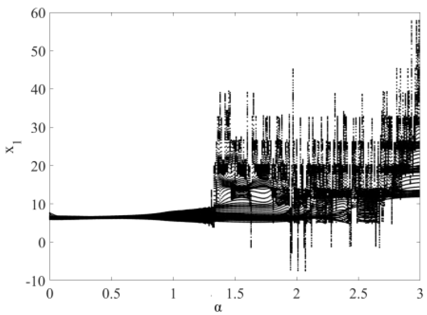
16], and step = 0.01 s. The bifurcation diagram of the disturbance amplitude
when the disturbance frequency does not change is shown in
Figure 1. The chaos phenomenon occurs in the system in cases where
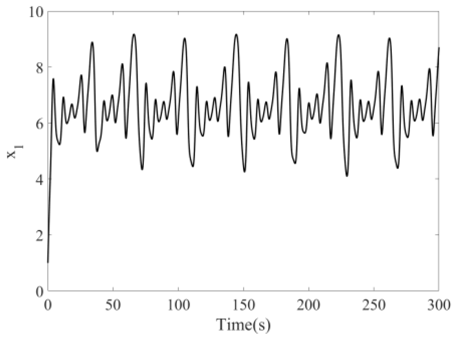
. The above initial values and parameters are still taken and
is used in the simulation to obtain
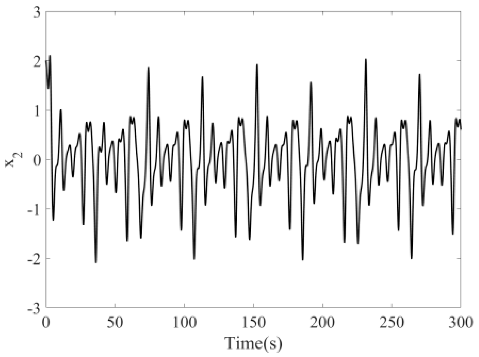
Figure 2 and
Figure 3, which show the time response diagrams of the state variables
and
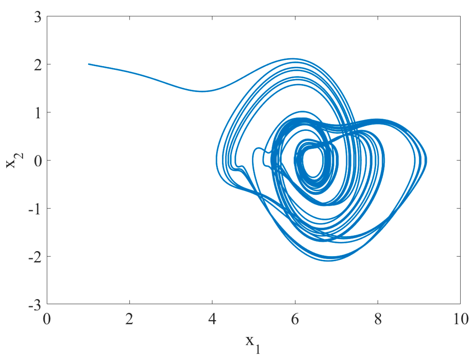
. As shown, the system is under an irregular operation state at this time. The phase diagram in
Figure 4 shows visible chaos status. The above information fully indicates that the system is under a chaotic status at this time.
This affects the operation reliability of the system and should be controlled. The following sections propose specific methods and strengths to control this chaos phenomenon.
3. The Application of Accurate Exponential Solution of a Differential Equation in Stability Control of One Class of Chaotic System with Known Parameters
This section describes an accurate exponential solution method of the differential equation, which can stably control one class of chaotic system with known parameters, make the global exponent of the system stable at the origin, and make it so that the convergence rate is easily adjusted. This method can eliminate the influences of the chaos phenomenon on the system.
3.1. Methods Proposed
Firstly, the disturbance term
of the system is removed from System
to obtain System
. We control System
firstly.
To control System
, the controller
is added as follows:
Before the system is controlled, one definition is given below. Definition 1 is a common sense definition.
Definition 1. Ifandexist andis satisfied, then Systemremains stable at the origin for any initial global exponent.
Theorem 1 is given according to the accurate exponential solution method of the differential equation.
Theorem 1. For the differential equation expressed by System, if the controller is The global exponent of System
remains stable at the origin, where
and
,
are the eigenvalues of the closed loop system given by Equations
and
.
Proof 1. To let System
make the global exponent stable at the origin, the solution of System
is assumed to be
where
and
are the constants related to the initial values.
because
and
. Since
, thus
and
is evident.
is obtained from System
Based on the above description, if the controller
exists in the form of Equation
, then System
has the following solution:
The solution of System is unique, Equation is the solution of System , and and ; thus, the global exponent of System remains stable at the origin.
is expressed as
and
in the following section. With Cramer’s Rule [
17], the following results are obtained from Equation
:
and
where the following results are found:
and
. They are substituted into Equation
, and the following equation is obtained:
which is the same as Equation
.
Take and let under the condition . According to Definition 1, the global exponent of System remains stable at the origin and the convergence speed is related to . The bigger the absolute value of is, the quicker the system’s convergence speed is. This cannot be embodied by a general control method and is one of the issues described in this paper along with the strength of this control algorithm. Theorem 1 is proved. □
3.2. Simulation Result
System
is simulated and validated according to Theorem 1. The initial values and parameters are defined as follows:
, and the step is 0.01 s.
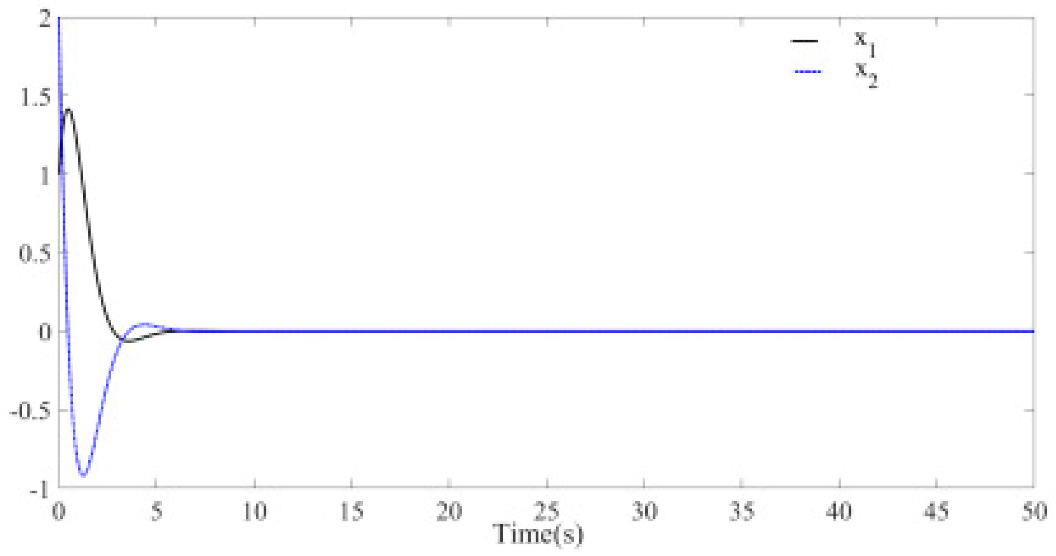
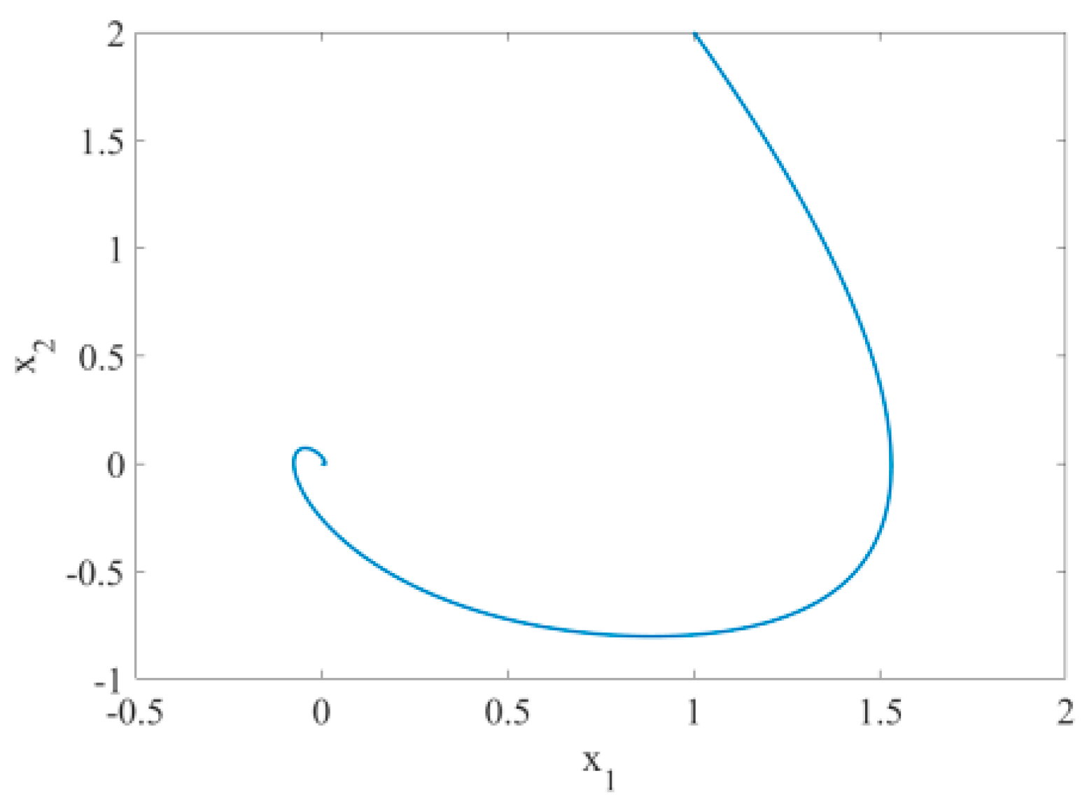
Figure 5 is the time response diagrams of the state variables
and
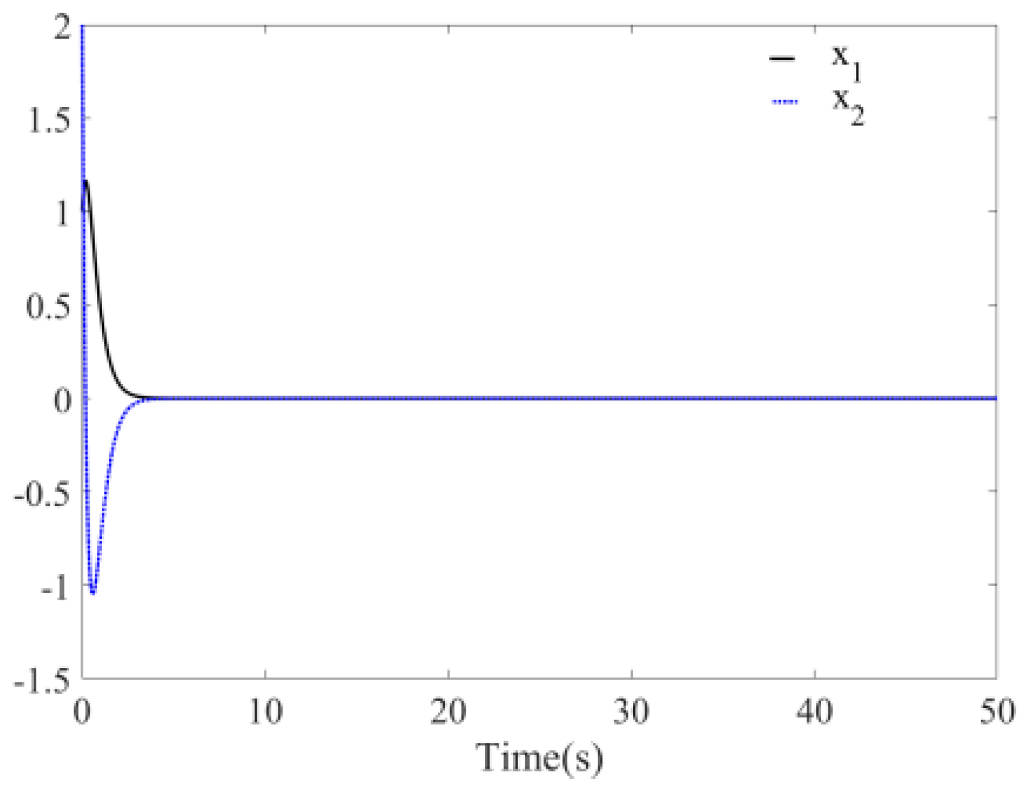
before disturbance is added to the system. The figure shows that the system remains stable at the origin at this time and the convergence time is about 8 s. If
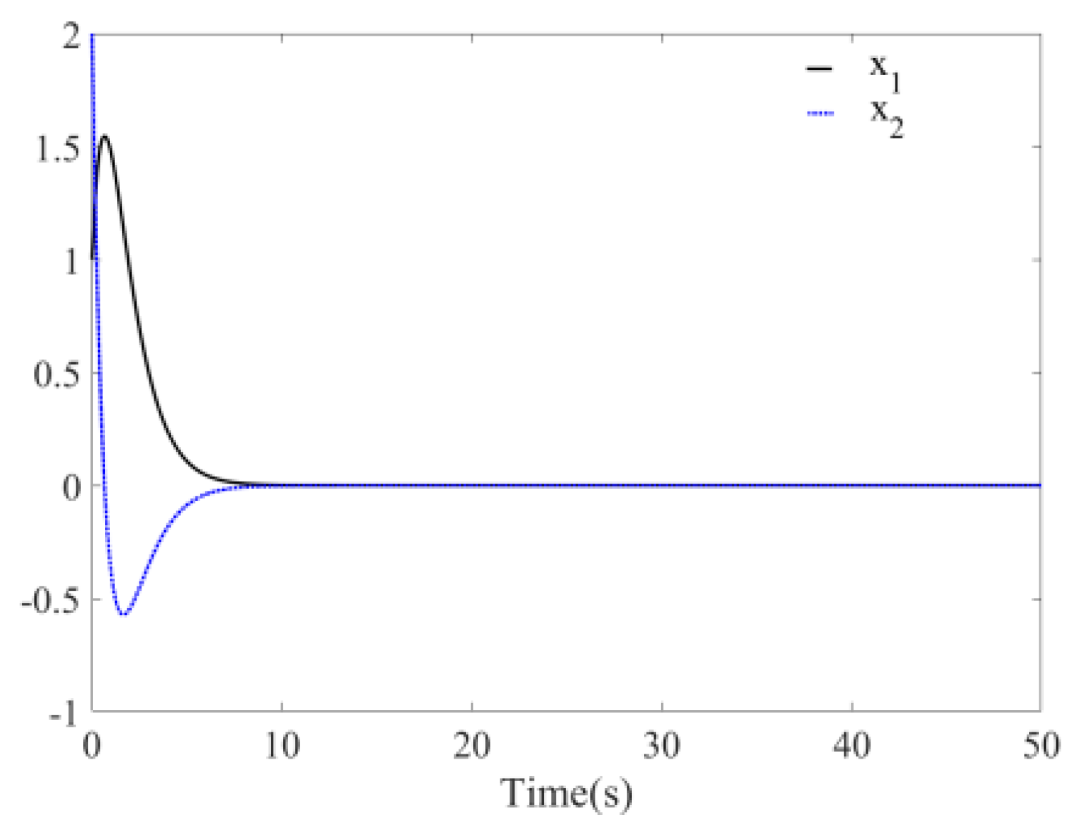
, the simulation figure changed to
Figure 6, the convergence time is 5 s. It can be seen that the convergence time can be controlled by parameters
and
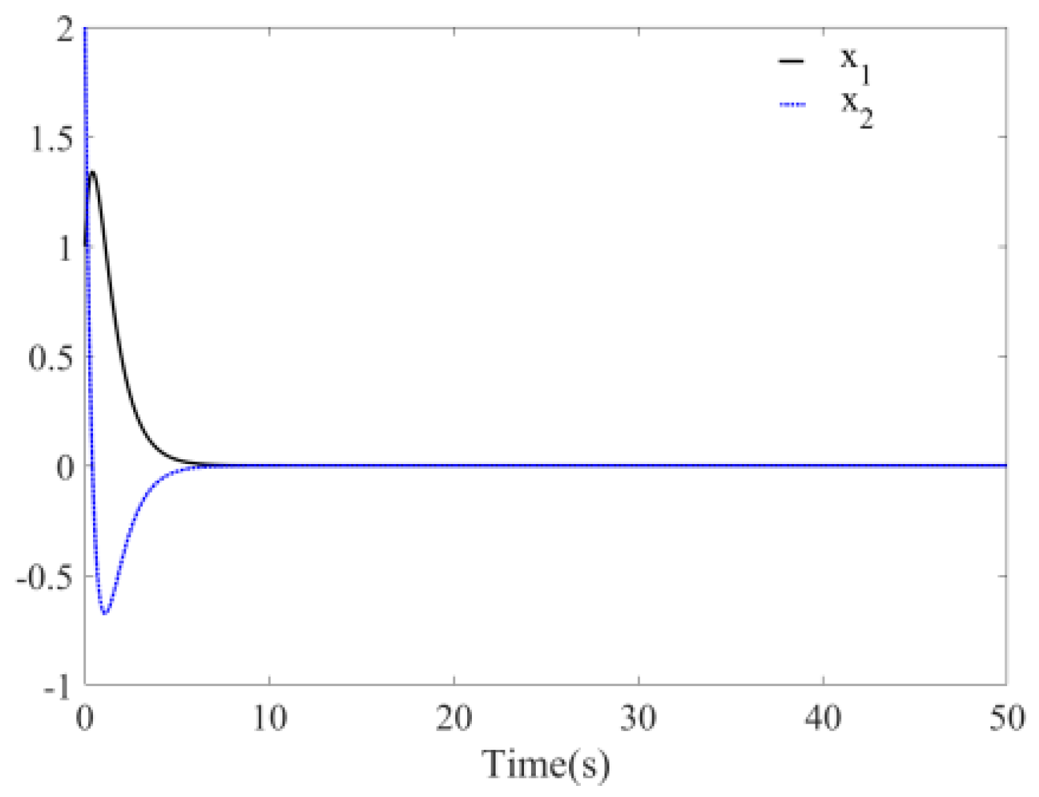
. The absolute value is bigger and the convergence time is smaller. From the phase diagram
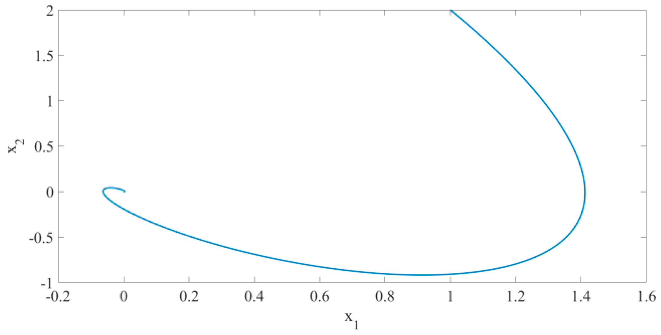
Figure 7, it is evident that the chaos phenomenon disappears and the system quickly remains stable at the origin. The above analysis indicates that the system without disturbance is globally exponentially stable at the origin.
In fact, the disturbance
has been removed in System
, and now we added it to the system as follows:
System
is simulated and validated according to above method. The initial values and parameters are defined as follows:
,
,
and the step is 0.01 s.
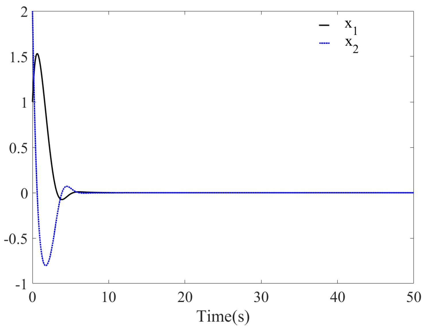
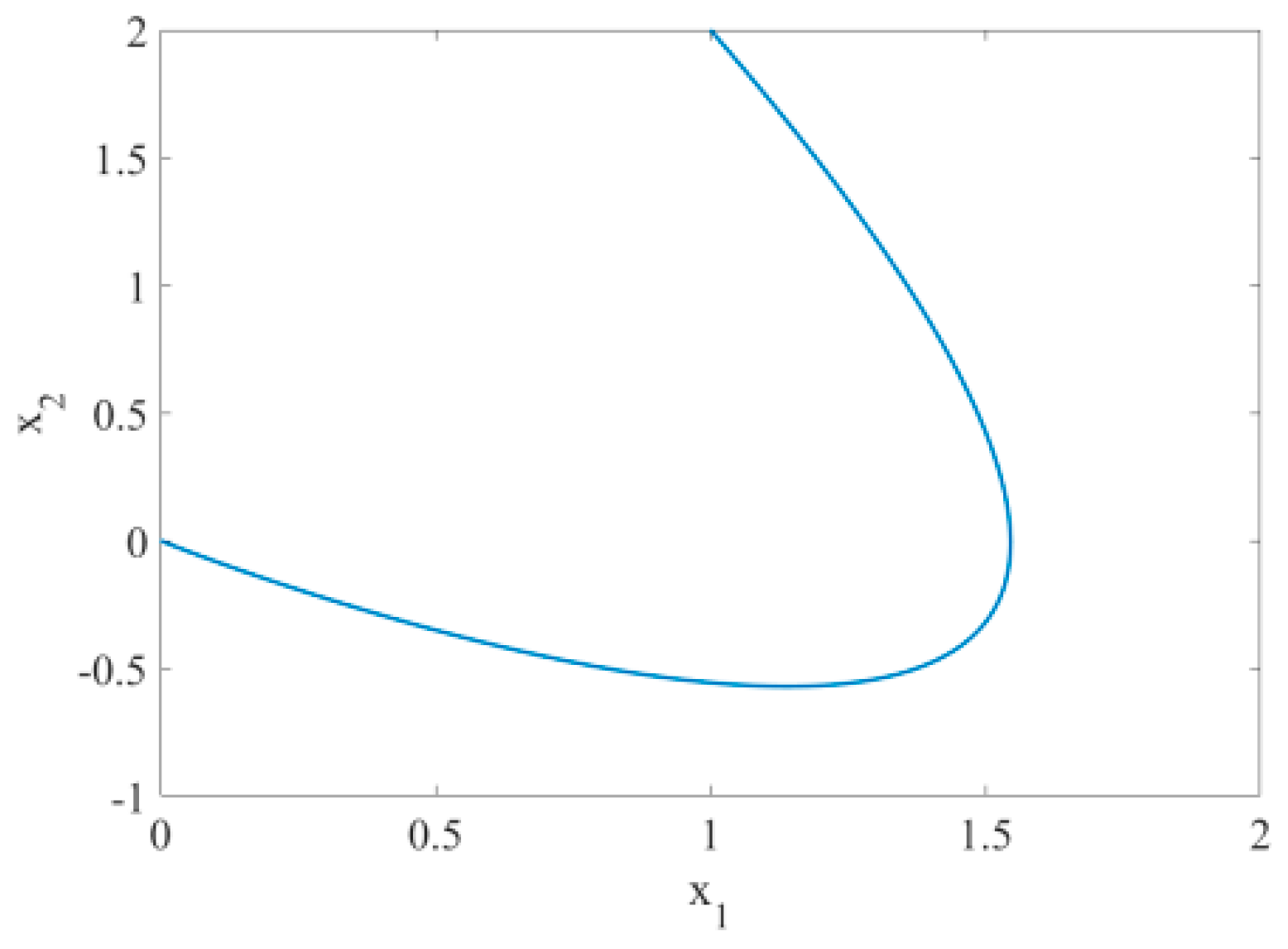
Figure 8 is the time response diagrams of the state variables
and
after disturbance is added to the system. The figure shows that the system still remains stable at the origin at this time and the convergence time is about 9 s. Compared with
Figure 5, the convergence time is 1 s more, the convergence trajectory is almost same, and the error can be accepted by one. From the phase diagram
Figure 9, it is evident that the system still remains stable at the origin. The above analysis indicates that the system with disturbance is globally exponentially stable at the origin, and it has good robustness.
Remark 1. The above controller depends greatly onand differenthave different controllers.
Remark 2. The Lyapunov function can be used to prove Theorem 1. The Lyapunov function is taken as follows:
, after Equations , , and are substituted, the following can be obtained: .
From the Lyapunov stability theorem, we can know that System remains globally stable at the origin. However, it is unknown whether the system converges at the origin exponentially in this case and whether the convergence rate is easy to adjust.
Remark 3. Many papers provide a control or synchronization method for the chaotic system, and the section above also proposed some control methods, but some common methods, such as a nonlinear method [18], an intermittent control method [19], and a state feedback control method [20], do not indicate whether the system converges at the origin exponentially and no method is given to adjust the convergence rate. However, the method in this paper gives conclusions. 4. The Application of Accurate Exponential Solution of a Differential Equation in Stability Control of One Class of Chaotic System with Unknown Parameters
Most research on chaos control is for known parameters, but some system parameters are generally designed based on complicated factors in the actual design and the system parameters vary in the actual system operation. Thus, control over the chaos system with unknown parameters is significant in practice. An accurate exponential solution control method of the differential equation is proposed for the chaos phenomenon with unknown parameters in the following section.
4.1. Methods Proposed
When unknown parameters exist in System
, the form is as follows:
where
and
indicate unknown parameters in the system.
Firstly, the system disturbance term
is removed from System
to obtain System
. We control System
firstly.
Theorem 2. After the controlleris added into System, the form is changed as follows:wherefor the differential equation in System, we use the controller:andwhereandare the estimated values ofand. At this time, Systemremained globally stable at the origin. Proof 2. From System
, one could obtain
Substituting Equation
to Equation
obtains
Take the Lyapunov function as
and then,
Substituting Equations
and
to Equation
obtains
System remains globally stable at the origin according to the Lyapunov stability theorem. Theorem 2 is proved. □
4.2. Simulation Result
System is simulated and validated according to Theorem 2 in the following part. The initial values and parameters are defined as follows:
,
, and the step is 0.01 s.
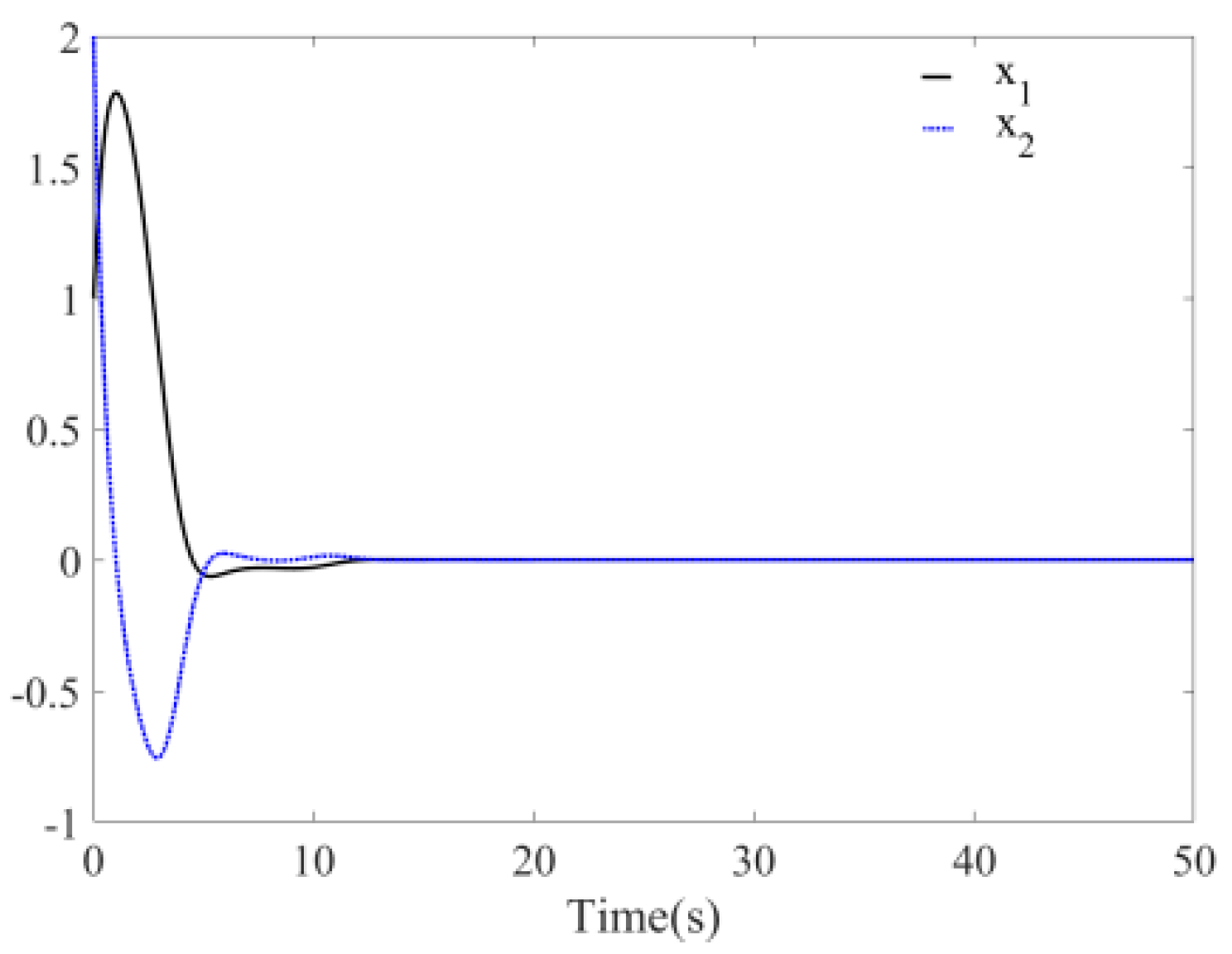
Figure 10 is the time response diagrams of the state variables
and
before disturbance is added to the system with unknown parameters. The figure shows that the system remains stable at the origin at this time and the convergence time is about 10 s. If
, the simulation figure changed to
Figure 11 and the convergence time is 8 s. It can be seen that the convergence time can be controlled by parameters
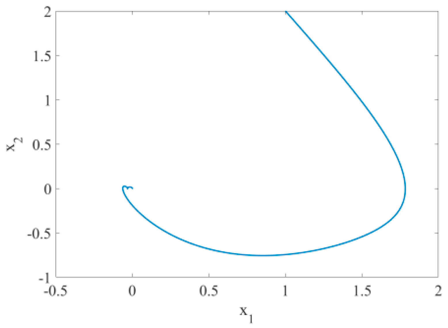
. The absolute value is bigger and the convergence time is smaller. From phase diagram
Figure 12, it is evident that the chaos phenomenon disappears and the system quickly remains stable at the origin.
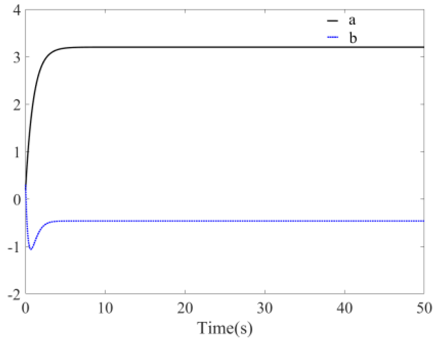
Figure 13 is the time response diagram of the two unknown parameters. The figure shows that two unknown parameters could quickly converge to the boundary values within 5 s.
The above information fully indicates that the system is free of the chaotic state and the global exponent remains stable at the origin. The unknown parameters identified the boundary values under the adaptation law. This indicates that the system is under control and the related unknown parameters are identified, which is significant in practice.
In fact, the disturbance
has been removed in System
, and now, we add it to the system as follows:
where
and
indicate unknown parameters in the system.
System
is simulated and validated according to above method. The initial values and parameters are defined as follows:
,
,
, and the step is 0.01 s.
Figure 14 is the time response diagrams of the state variables
and
after disturbance is added to the system with unknown parameters. The figure shows that the system still remains stable at the origin at this time and the convergence time is about 13 s. Compared with
Figure 10, the convergence time is 3 s more and the convergence trajectory and the error can be accepted by one. From the phase diagram
Figure 15, it is evident that the system still remained stable at the origin.
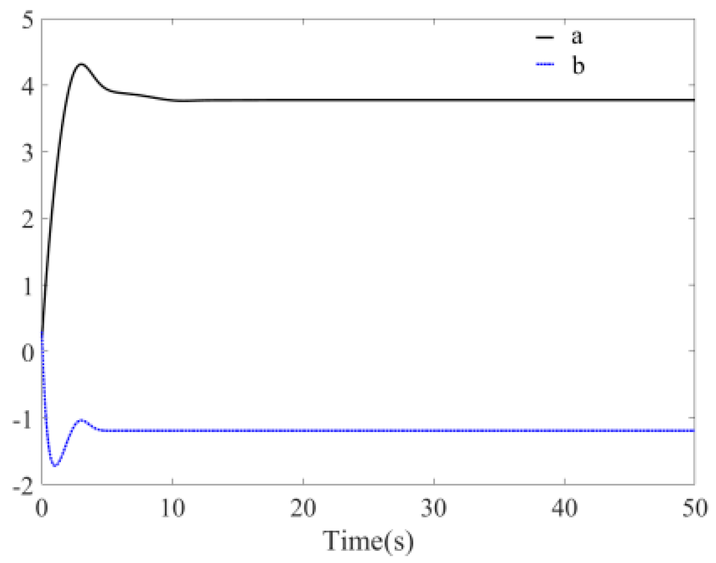
Figure 16 is the time response diagram of the two unknown parameters. The figure shows that two unknown parameters could quickly converge to the boundary values within 8 s.
The above analysis indicates that the chaotic system with disturbance and unknown parameters is globally exponentially stable at the origin, the unknown parameters can be identified, the convergence rate can be adjusted by parameter , and it has good robustness.
5. The Application of Ship’s Electric Chaotic System
The following is a brief introduction to the application of the model mentioned above, taking the ship’s electric chaotic system as an example.
The ship’s electric system is an enclosed system in most cases and has no association with the outside world. Two machines are connected in parallel, which is the foundation of multi-machine complicated systems. The multi-machine system analysis can be extended from the two-machine system and plentiful complicated systems can be discussed as equivalent two-machine systems. Thus, chaos control of the two-machine system has universal meaning [
21]. When electronic disturbances exist, assuming that a machine is an infinite bus system, the basic model is as follows:
where
is the operating angle of the generator rotor,
is the operating angular velocity of the motor rotor,
is the input mechanical power,
is the output electric power,
is the damped coefficient,
is the moment of inertia,
is the amplitude of electromagnetic power disturbance, and
is the disturbance frequency of the electromagnetic power [
16].
Let
and then,
where
, let
and
, and then,
It can be seen that Formula is the same as Formula , so the method mentioned in this paper can be applied to a ship’s electric chaos control and can be further studied.
6. Conclusions
In this paper, an accurate exponential solution method of the differential equation is used to study the exponential stabilization of one class of chaotic system; control the chaos phenomenon under certain conditions; avoid harming systems, such as splitting and crash-down; and guarantee reliable operation. The method used in this paper has the following strengths: the solution can be designed to exponentially converge to the origin and the convergence rate can be easily adjusted, namely, several known parameters can be adjusted and set with proper values in advance for quick convergence. The simulation data show that the chaos phenomenon of the controlled chaotic system disappears and the system quickly converges to the origin in an exponential manner. Based on this, the chaotic system with unknown parameters is stably controlled, unknown parameters are identified, and the system could quickly converge to the boundary values under control of the adaptation law. The above analysis fully proves that the proposed control method is effective. It is found that the ship’s electric system has the same model, which has more practical significance.
Author Contributions
Conceptualization, C.G.; methodology, H.J.; software, H.J.; validation, H.J.; formal analysis, H.J.; resources, H.J.; data curation, H.J.; writing—original draft preparation, H.J.; writing—review and editing, H.J.; supervision, C.G.; project administration, C.G.; funding acquisition, C.G. All authors have read and agreed to the published version of the manuscript.
Funding
This research was funded by the National Natural Science Foundation of China, grant number 51809028, grant number 51579024, and grant number51879027.
Conflicts of Interest
The authors declare no conflict of interest.
References
- Junhai, H.; Yunjie, W.U. Survey on Chaos control. Comput. Simul. 2006, 23, 6–8. [Google Scholar]
- Chen, L. Ship Power System Prediction Model Based on Chaos Theory. Master’s Thesis, The Wuhan University, Wuhan, China, 2011; pp. 21–23. [Google Scholar]
- Ma, M. Research on Chaos Control of Ship Power System. Master’s Thesis, The Harbin Engineering University, Harbin, China, 2010; pp. 6–8. [Google Scholar]
- Li, Y.; Wang, H.; Tian, Y. Fractional-order adaptive controller for chaotic synchronization and application to a dual-channel secure communication system. Mod. Phys. Lett. B 2019, 33. [Google Scholar] [CrossRef]
- Mohanty, N.P.; Dey, R.; Roy, B.K. Switching synchronisation of a 3-D multi-state-time-delay chaotic system including externally added memristor with hidden attractors and multi-scroll via sliding mode control. Eur. Phys. J. Spec. Top. 2020, 229, 1231–1244. [Google Scholar] [CrossRef]
- Wang, J.; Liu, L.; Liu, C.; Li, X. Adaptive sliding mode control based on equivalence principle and its application to chaos control in a seven-dimensional power system. Math. Probl. Eng. 2020, 2020, 1565460. [Google Scholar] [CrossRef]
- Wang, B.; Chen, L.L. New results on fuzzy synchronization for a kind of disturbed memristive chaotic system. Complex 2018, 2018, 3079108. [Google Scholar] [CrossRef]
- El-Gohary, A. Optimal synchronization of Rössler system with complete uncertain parameters. Chaos Solitons Fractals 2006, 27, 345–355. [Google Scholar] [CrossRef]
- Ablay, G. Chaos in PID controlled nonlinear systems. J. Electr. Eng. Technol. 2015, 10, 1843–1850. [Google Scholar] [CrossRef] [Green Version]
- Panaitescu, F.; Panaitescu, M.; Deleanu, D.; Anton, I.A. Analysis of environmental risk and extreme roll motions for a ship in waves. J. Environ. Prot. Ecol. 2019, 20, 1204–1213. [Google Scholar]
- Yao, Q.; Su, Y.; Li, L. Application of Negative Feedback Control Algorithm in Controlling Nonlinear Rolling Motion of Ships. In Proceedings of the 7th International Conference on Advanced Materials and Computer Science (ICAMCS 2018), Dalian, China, 21–22 December 2018; pp. 88–94. [Google Scholar]
- Nara, S.; Soma, K.-I.; Yamaguti, Y.; Tsuda, I. Constrained chaos in three-module neural network enables to execute multiple tasks simultaneously. Neurosci. Res. 2020, 156, 217–224. [Google Scholar] [CrossRef] [PubMed]
- Chen, Y.S.; Hwang, R.R.; Chang, C.C. Adaptive impulsive synchronization of uncertain chaotic systems. Phys. Lett. A 2010, 374, 2254–2258. [Google Scholar] [CrossRef]
- Geiselhart, R. Lyapunov functions for discontinuous difference inclusions. 10th IFAC Symposium on Nonlinear Control Systems (NOLCOS). IFAC PapersOnLine 2016, 49, 223–228. [Google Scholar] [CrossRef]
- Zhou, L.; Chen, F. Subharmonic bifurcations and chaotic dynamics for a class of ship power system. J. Comput. Nonlinear Dyn. 2018, 13, 031011. [Google Scholar] [CrossRef]
- Huang, J. Study on Chaos of Ship Power System. Master’s Thesis, The Shanghai Maritime University, Shanghai, China, 2005; pp. 29–34. [Google Scholar]
- Song, G.-J.; Yu, S.-W. Cramer’s rule for the general solution to a restricted system of quaternion matrix equations. Adv. Appl. Clifford Algebras 2019, 29, 91. [Google Scholar] [CrossRef]
- Mukherjee, M.; Halder, S. Stabilization and control of chaos based on nonlinear dynamic inversion. Energy Procedia 2017, 117, 731–738. [Google Scholar] [CrossRef]
- Sang, H.; Zhao, J. Exponential Synchronization and L2-Gain Analysis of Delayed Chaotic Neural Networks Via Intermittent Control WITH Actuator Saturation. Transactions on Neural Networks and Learning Systems; Institute of Electrical and Electronics Engineers (IEEE): Piscataway, NJ, USA, 2019; Volume 30, pp. 3722–3734. [Google Scholar]
- Ding, K. Master-Slave Synchronization of Chaotic Φ6 Duffing Oscillators by Linear State Error Feedback Control. Complex 2019, 2019, 1–10. [Google Scholar] [CrossRef] [Green Version]
- Cheng, P.; Liang, N.; Li, R.; Lan, H.; Cheng, Q. Analysis of Influence of Ship Roll on Ship Power System with Renewable Energy. Energies 2020, 13, 1. [Google Scholar] [CrossRef] [Green Version]
Figure 1.
Bifurcation diagram of chaotic System ().
Figure 1.
Bifurcation diagram of chaotic System ().
Figure 2.
Time response of .
Figure 2.
Time response of .
Figure 3.
Time response of .
Figure 3.
Time response of .
Figure 4.
Phase diagram of chaotic System .
Figure 4.
Phase diagram of chaotic System .
Figure 5.
Time response of system with known parameters (without disturbance, ).
Figure 5.
Time response of system with known parameters (without disturbance, ).
Figure 6.
Time response of system with known parameters (without disturbance, ).
Figure 6.
Time response of system with known parameters (without disturbance, ).
Figure 7.
Phase diagram of system with known parameters (without disturbance, ).
Figure 7.
Phase diagram of system with known parameters (without disturbance, ).
Figure 8.
Time response of system with known parameters (with disturbance, ).
Figure 8.
Time response of system with known parameters (with disturbance, ).
Figure 9.
Phase diagram of system with known parameters (with disturbance, ).
Figure 9.
Phase diagram of system with known parameters (with disturbance, ).
Figure 10.
Time response of system with unknown parameters (without disturbance, ).
Figure 10.
Time response of system with unknown parameters (without disturbance, ).
Figure 11.
Time response of system with unknown parameters (without disturbance, ).
Figure 11.
Time response of system with unknown parameters (without disturbance, ).
Figure 12.
Phase diagram of system with unknown parameters (without disturbance, ).
Figure 12.
Phase diagram of system with unknown parameters (without disturbance, ).
Figure 13.
Identification of unknown parameters and (without disturbance, ).
Figure 13.
Identification of unknown parameters and (without disturbance, ).
Figure 14.
Time response of system with unknown parameters (with disturbance, ).
Figure 14.
Time response of system with unknown parameters (with disturbance, ).
Figure 15.
Phase diagram of system with unknown parameters (with disturbance, ).
Figure 15.
Phase diagram of system with unknown parameters (with disturbance, ).
Figure 16.
Identification of unknown parameters and (with disturbance, ).
Figure 16.
Identification of unknown parameters and (with disturbance, ).
© 2020 by the authors. Licensee MDPI, Basel, Switzerland. This article is an open access article distributed under the terms and conditions of the Creative Commons Attribution (CC BY) license (http://creativecommons.org/licenses/by/4.0/).


