Predicting Primary Energy Consumption Using Hybrid ARIMA and GA-SVR Based on EEMD Decomposition

Abstract

Forecasting energy consumption is not easy because of the nonlinear nature of the time series for energy consumptions, which cannot be accurately predicted by traditional forecasting methods. Therefore, a novel hybrid forecasting framework based on the ensemble empirical mode decomposition (EEMD) approach and a combination of individual forecasting models is proposed. The hybrid models include the autoregressive integrated moving average (ARIMA), the support vector regression (SVR), and the genetic algorithm (GA). The integrated framework, the so-called EEMD-ARIMA-GA-SVR, will be used to predict the primary energy consumption of an economy. An empirical study case based on the Taiwanese consumption of energy will be used to verify the feasibility of the proposed forecast framework. According to the empirical study results, the proposed hybrid framework is feasible. Compared with prediction results derived from other forecasting mechanisms, the proposed framework demonstrates better precisions, but such a hybrid system can also be seen as a basis for energy management and policy definition.

1. Introduction

Research on energy supply and demand has become critical since the 1973 oil crisis. In the past decades, the average annual worldwide energy consumption grew due to the rapid economic growth of major economies. Based on the forecast by BP [1], the worldwide energy consumption will increase by 34% between 2014 and 2035. Over 90% of the world’s energy consumption comes from coal, oil, natural gas, and nuclear sources [1]. Furthermore, energy consumption always plays a dominant role in countries’ long-term sustainability. For most industries, e.g., heavy industries, much more energy will be required for sustainable growth. Therefore, the understanding and prediction of energy consumption in general, and of a specific economy in particular, are critical from an economic perspective.

Recently, scholars have started to forecast the demand and supply of energy by integrating various models into a hybrid one [2,3,4]. In general, such hybrid forecasting methods can be divided into two: causal models and time series models. On the one hand, causal models are mainly constructed based on one or more independent variables. Then the dependent variables can be predicted. Strict assumptions and theoretical bases are required for constructing such causal models. On the other hand, time series models are based on historical data. Whether linear or nonlinear, such models are used for estimating future values. These approaches are always regarded as the most feasible ways to predict energy consumption. The fundamental purpose of time series is to derive trends or patterns that can be modeled by econometric methods such as the autoregressive integrated moving average (ARIMA). However, the models for nonlinear time series predictions are always difficult to realize due to the uncertainty and volatility of the time series. Since the linear models cannot be used to predict complex time series, nonlinear approaches are more suitable for such purpose. Thus, this study aims to predict energy consumption by using integrated methods that incorporate linear and nonlinear methods. Due to issues that arise in time series forecasting, accurate predictions are essential. Conventional linear approaches are effective in the event of forecasting issues. However, more studies are finding that, compared to nonlinear methods, such as support vector machines (SVMs) and tree-based algorithms, linear methods do not perform well in the event of various time series problems, especially complex time sequences. This is because linear methods cannot be used to detect the complex implicit patterns in time series. This study adopts a hybrid model by incorporating linear and nonlinear methods to predict energy consumption and overcome this problem.

However, in accordance with previous studies, no single prediction model is applicable to all scenarios. Therefore, many researchers have introduced hybrid models for predicting time series; such models incorporate both linear and nonlinear models or combine two linear models [5]. Earlier works have also revealed that such hybridization of prediction frameworks not only shows the complementary nature of the frameworks with respect to predictions but also enhances the accuracy of predictions. Thus, models in hybrid forms have become a common practice in forecasting. However, noise and unknown factors exist in time series. These factors influence the volatility of time series and cannot be easily solved by hybridizing linear and nonlinear patterns only. Such hybridization probably produces an overfitting problem; thus, the optimal parameters required to model a prediction framework cannot be derived. Fortunately, such difficulties can be partially solved by leveraging the ensemble empirical mode decomposition (EEMD) proposed by Wu and Huang [6] because the EEMD can solve the noise problems and enhance the prediction performance. Noises, such as trend, seasonality, and unknown factors, which often exist in time series, influence forecasting performance. To make the prediction more precise, noise problems should be carefully dealt with. There are several ways to approach noise problems and enhance forecasting performance. One way is to tune the hyperparameter for algorithms (such as the support vector regression, SVR). As a result, the prediction’s performance will improve. Another way is to first deal with the time sequence using a decomposition method, such as the EEMD method. If a decomposition approach is used, the time series can be split into several stable sequences for prediction. The more stable the sequences, the better the model’s prediction performance. The feasibility of EEMD has been verified by various works (e.g., [7,8]) in solving nonstationary time series and complex signals.

Given the abovementioned advantages regarding the advantages of the hybrid prediction system as well as the EEMD for time series, this research proposes a novel hybrid framework integrating the EEMD, ARIMA, genetic algorithm (GA), and the SVR to predict primary energy consumption. The concept of the proposed model comes from several sources. First, in conventional time series methods, ARIMA is popular and powerful. It has been extensively used to deal with various forecasting issues. Therefore, the ARIMA method is suitable for this study. Second, based on past research, univariate or single methods used to deal with forecasting problems cannot yield a high forecasting performance when compared to hybrid methods. Therefore, this study simultaneously uses another nonlinear method, SVR, to enhance the prediction performance. In past decades, SVR has been useful in a wide variety of prediction domains. Therefore, SVR is suitable for this study. Although SVR has obtained several important prediction records, it has a significant problem: hyperparameter tuning. Hyperparameter tuning will affect forecasting performance. It is thus necessary to find a way to select the ideal hyperparameter for SVR. Due to computing speed, the authors cannot spend much time searching for the ideal hyperparameters. Consequently, the greedy algorithm (grid search) will be abandoned. Instead, the authors intend to adopt a heuristic algorithm, such as the GA approach, to find the best hyperparameters in SVR. Finally, decomposition methods’ effectiveness in enhancing models’ forecasting performance has been verified by past literature. The EEMD, Wavelet, and other methods have been hugely successful in the signal processing field. Due to the innovativeness and power of EEMD, recent studies have widely adopted the method in signal processing research.

Based on above-mentioned reasons, the authors attempt to combine the EEMD, ARIMA, GA, and SVR into a prediction model for energy consumption. First, the time series of energy consumption is divided into several intrinsic mode functions (IMFs) and a residual term. Here, IMFs stand for different frequency bands of time series, which range from high to low, while each IMF represents a series of oscillatory functions [9,10]. That way, each time series component can be identified and modeled accordingly. The characteristics of the time series can also be captured in detail. The ARIMA is then introduced to predict the future values of all extracted IMFs and the residue independently. Since the accuracy of the nonlinear time series derived using the ARIMA may be unacceptable, the SVR is utilized based on the nonlinear pattern to further improve prediction performance. In addition, the accuracy of the SVR-based prediction models completely depends on the control parameters, and the parameters should be optimized. Therefore, the GA is leveraged to derive the optimal parameters. In general, the prediction model fuses EEMD, ARIMA, SVR, and GA into a hybrid prediction framework. The predicted IMFs and the residue will be split into a final ensemble result. The proposed hybrid framework will be verified by a prediction of Taiwanese primary energy consumption for the next four years. Meanwhile, the accuracy of the prediction results will be compared with the ones derived by other forecast methods, which include ARIMA, ARIMA-SVR, ARIMA-GA-SVR, EEMD-ARIMA, EEMD-ARIMA-SVR, and EEMD-ARIMA-GA-SVR. Based on the empirical study results, the effectiveness of the prediction framework can be verified.

The remaining part of this work is structured as follows. Section 2 reviews the related literature regarding the consumption and forecasting methods of energy. Section 3 introduces the methods used in this paper, which include ARIMA, SVR, and GA. Section 4 describes the background of the empirical study case, the dataset, and the empirical study process. Section 5 concludes the whole work, with major findings and opportunities for future studies.

2. Literature Review

For decision-makers to effectively understand the trend of energy fluctuation, which may generate far-reaching implications, the precise forecasting of primary energy consumption is indispensable. On the one hand, with an accurate forecasting of energy consumption, the government can establish energy plans for fluctuations in oil supply. On the other hand, energy predictions can be useful for the investment of firms. Albeit important, predicting energy consumption is not always simple. Therefore, a robust forecasting model will be necessary.

In the literature on energy prediction, several researchers have completed accurate predictions [2,3,4,11,12]. Some researchers adopted economic indicators by mixing various energy indicators for predicting energy consumption. Other researchers used only time series data for forecasting. While these forecast methods are different, the prediction results of the two categories of models can serve as solid foundations for further investigations on energy consumption.

Furthermore, to enhance the accuracy of predictions, some authors employed hybrid models. Of such models, linear and nonlinear ones were integrated. The fusion of linear and nonlinear models can overcome the shortage of adopting only one kind of method and provide more accurate results [3,5,13]. In addition to the hybrid methods involving both linear and nonlinear models, some studies have attempted to transform the data by integrating data preprocessing and post-processing procedures [14,15]. By doing so, the forecasting capabilities of the hybrid models with data preprocessing and postprocessing procedures can show superior performance in energy predictions.

Further, several studies have proposed machine learning methods for predicting energy consumption. Al-Garni, Zubair, and Nizami [16] used weather factors as explanatory variables of a regression model for predicting the consumption of electric energy in eastern Saudi Arabia. Azadehet al. [12] modeled Turkey’s electricity consumption on the sector basis by utilizing the artificial neural network (ANN). Wong, Wan, and Lam [17] developed an ANN-based model for analyzing the energy consumption of office buildings. Fumo and Biswas [11] employed simple and multiple regression models as well as the quadratic regression model to predict residential energy consumption. Ahmadet al. [13] attempted to review the applications of ANN and the SVM for energy consumption prediction and found that both seem to show better performance in energy forecasting [13]. Ardakani and Ardehali [3] applied regressive methods consisting of linear, quadratic, and ANN models by incorporating an optimization algorithm into the model to achieve better performance in predicting long-term energy consumption.

Although many scholars have empirically verified the effectiveness of machine learning methods for dealing with time series problems, no single prediction model seems applicable to all scenarios. That is, even if the machine learning model outperforms other traditional linear methods, using a single machine learning model to address all time series issues would be problematic and unrealistic.

Many researchers have thus employed hybrid time series forecasting models, which incorporate linear with nonlinear models or combine two kinds of linear models [5]. Previous studies have also revealed that such hybrid frameworks not only complement each other in prediction but also enhance prediction accuracy. Thus, models in hybrid forms have become a common practice in forecasting.

For example, Yuan and Liu [2] proposed a composite model that combined ARIMA and the grey forecasting model, GM (1,1), to predict the consumption of primary energy in China. Based on their findings, the results obtained when using the hybrid model were far superior to those obtained when only using the ARIMA or GM (1,1) models. Zhang [18] developed a hybrid prediction model consisting of both ARIMA and ANN. Zhu et al. [4] developed a hybrid prediction model of energy demands in China, which employed the moving average approach by integrating the modified particle swarm optimization (PSO) method for enhancing prediction performance. Wang, Wang, Zhao, and Dong [19] combined the PSO with the seasonal ARIMA method to forecast the electricity demand in mainland China and obtain a more accurate prediction. Azadeh, Ghaderi, Tarverdian, and Saberi [20] also adopted the GA and ANN models to predict energy consumption based on the price, value-add, number of customers, and energy consumption. Lee and Tong [21] proposed a model that combined ARIMA and genetic programming (GP) to improve prediction efficiency by adopting the ANN and ARIMA models.

Further, Yolcuet et al. [5] developed a linear and nonlinear ANN model with the modified PSO approach for time series forecasting. They achieved prediction results superior to those of conventional forecasting models. According to the analytical results, the hybrid model is more effective because it adopts a single prediction method and can thus improve the prediction accuracy.

Though hybrid models based on ARIMA and ANN have achieved great success in various fields, they have several limitations. First, this hybrid approach requires sufficient data to build a robust model. Second, the parameter control, uncertainties in weight derivations, and the possibility of overfitting must often be discussed when using ANN models. Because of these limitations, more researchers started to adopt SVR in forecasting since it can mitigate the disadvantages of ANN models. SVR is suitable for forecasts based on small datasets.

Pai and Lin’s [22] work is a representative example of adopting SVR methods in hybrid models for forecasting. They integrated ARIMA and SVR models for stock price predictions. Patel, Chaudhary, and Garg [23] also adopted the ARIMA-SVR for predictions and derived optimal results based on historical data. Alwee, Hj Shamsuddin, and Sallehuddin [24] optimized an ARIMA-SVR-based model, using the PSO for crime rate predictions. Fan, Pan, Li, and Li [25] employed independent component analysis (ICA) to examine crude oil prices and then used an ARIMA-SVR-based model to predict them.

Based on the results of the literature review, hybrid models, including both the SVR and the ANN, have achieved higher prediction accuracies than traditional prediction techniques. However, the invisible and unknown factors which can influence the volatility of time series cannot be addressed easily by hybridizing linear and nonlinear patterns. The problem of overfitting can emerge; thus, the optimal parameters cannot be derived.

Fortunately, such difficulties can be partially resolved by leveraging the EEMD proposed by Wu and Huang [6]. The method has been feasible and effective in solving problems consisting of nonstationary time series and complex signals [7,8]. Wang et al. [7] integrated the EEMD method with the least square SVR (LSSVR) and successfully predicted the time series of nuclear energy consumption. Prediction performance has increased significantly and outperformed some well-recognized approaches based on level forecasting and directional prediction. Zhang, Zhang, and Zhang [26] predicted the prices of crude oil by hybridizing PSO-LSSVM and EEMD decomposition. The work demonstrated that the EEMD technique can decompose the nonstationary and time-varying components of times series of crude oil prices. The hybrid model can be beneficial to model the different components of crude oil prices and enhance prediction performance.

The previous studies in the literature review section aimed to develop a model that could effectively and accurately predict energy consumption and demand. In their methodologies, these works being reviewed attempted to use linear or nonlinear methods to predict energy consumption. Furthermore, they tried to use the parameter search algorithm in their model to enhance its prediction accuracy. Based on the review results, complex time series can be split by the EEMD into several relatively simple subsystems. The hidden information behind such complex time series can be explored more easily. Thus, in the following section, a hybrid analytical framework consisting of ARIMA, SVR, and GA will be proposed. The framework will be adopted to predict primary energy consumption.

3. Research Methods

This section first introduces the data processing method. Next, the individual models including ARIMA and SVR will be introduced. Afterward, the optimization approach based on GA will be introduced. Finally, the analytical process of the proposed hybrid model will be described.

3.1. EEMD

Empirical mode decomposition (EMD), an adaptive approach based on the Hilbert–Huang transformation (HHT), is often used to deal with time series data including ones with nonlinear and nonstationary forms [8]. Since such time series are complicated, various fluctuation modes may coexist. The EMD technique can be used to decompose the original time series into several simple IMFs, which correspond to different frequency bands of the time series and range from high to low; each IMF stands for a series of oscillatory functions [9,10]. Moreover, the IMFs must satisfy two conditions [6]: (1) in the whole data series, the number of extrema and zero crossings must either be equal or differ at most by 1; and (2) at any point, the mean value of the envelope (envelope, in mathematics, is a curve that is tangential to each one of a family of curves in a plane) defined by the local minima is 0.

Based on the above definitions, IMFs can be extracted from the time series $y(t)$ according to the following shifting procedures [27]: (1) identify the local maxima and the minima; (2) connect all local extrema points to generate an upper envelope $e_{max}(t)$ and connect all minima points to generate a lower envelope $e_{min}(t)$ with the spline interpolation, respectively; (3) compute the mean of the envelope, $a(t)$, from the upper and lower envelopes, where $a(t)=(e_{max}(t)+e_{min}(t))/2$; (4) extract the mean from the time series and define the difference between $y(t)$ and $a(t)$ as $c(t)$, where $c(t)=y(t)-a(t)$; (5) check the properties of $c(t)$: (i) if $c(t)$ satisfies the two conditions illustrated above, an IMF will be extracted and replace $y(t)$ with the residual, $r(t)=y(t)-c(t)$; (ii) if $c(t)$ is not an IMF, then $y(t)$ will be replaced by $c(t)$; and (6) the residue $r_1(t)=y(t)-c_1(t)$ is regarded as the new data subjected to the same shifting process, which was described above for the next IMF from $r_1(t)$. When the residue $r(t)$ becomes a monotonic function or at most has one local extrema point from which no more IMF can be extracted [27], the shifting processes can be terminated.

Through the abovementioned shifting process, the original data series $y(t)$ can be expressed as a sum of IMFs and a residue, $y(t)={\displaystyle \sum _{i=1}^m{c}_i(t)}+r_m(t)$, where $m$ is the number of IMFs, $r_m(t)$ is the final residue, and $c_i(t)$ is the ith IMF. All the IMFs are nearly orthogonal to each other, and all have nearly zero means.

Although the EMD has been widely adopted in handling data series, the mode-mixing problem still exists. The problem can be defined as either a single IMF consisting of components of widely disparate scales or a component of a similar scale residing in different IMFs. To overcome this problem, Wu and Huang [6] proposed the ensemble EMD (EEMD), which adds white noise to the original data, and thus the data series of different scales can be automatically assigned to proper scales of reference built by the white noise [7]. The core concept of the EEMD method is to add the white noise into the data processing. White noise can be viewed as a sequence with zero mean value; this sequence does not fall under any distribution. Based on different algorithms, the white noise can be assigned to specific distributions for calculation. In EEMD, the purpose of this method is to make the original sequence the stable sequence. Hence, this method employs simulation, using the original sequence to generate various sequences of normal distributions—this is the white noise concept. With this method, the original sequence can be split into several different sequences. Meanwhile, the sum of the decomposed sequences equals the original sequence. These decomposed sequences are called IMFs. This way, the mode-mixing problem can be easily solved. The EEMD procedure is developed as follows [6]: (1) add a white noise series to the original data; (2) decompose the data with added white noise into IMFs; (3) repeat steps 1 and 2 iteratively, but with different white noise each time; and (4) obtain ensemble means of corresponding IMFs as the final results.

In addition, Wu and Huang [6] established a statistical rule to control the effect of added white noise: $e_n=\epsilon /\sqrt{n}$, where $n$ is the number of ensemble members, $\epsilon$ represents the amplitude of the added noise, and $e_n$ is the final standard deviation of error, which is defined as the difference between the input signal and the corresponding IMFs. Based on previous studies, the number of ensemble members is often set to 100, and the standard deviation of white noise is set to 0.2.

3.2. The ARIMA Model

The ARIMA model for forecasting time series was proposed by Box, Jenkins, and Reinsel [28]. The model consists of the autoregressive (AR) and the moving average (MA) models. The AR and MA models were merged into the ARMA model, which has already become matured in predictions. The future value of a variable is a linear function of past observations and random errors. Thus, the ARMA can be defined as

$$y_t={\varphi }_1{y}_{t-1}+{\varphi }_2{y}_{t-2}+\cdots +{\varphi }_p{y}_{t-p}+{\epsilon }_t-{\theta }_1{\epsilon }_{t-1}-{\theta }_2{\epsilon }_{t-2}-\cdots -{\theta }_q{\epsilon }_{t-q}$$

(1)

where $y_t$ is the forecasting value; ${\varphi }_i$ is the coefficient of the ith observation; $y_{t-i}$ is the ith observation; ${\theta }_i$ is the parameter associated with the ith white noise; ${\epsilon }_t$ is the white noise, whose mean is zero; and ${\epsilon }_{t-i}$ is the noise terms.

The ARMA model can satisfactorily fit the original data when the time series data is stationary. However, if the time series are nonstationary, the series will be transformed into a stationary time series using the dth difference process, where $d$ is usually set as 0, 1, or 2. ARIMA is used to model the differenced series. The process is called ARIMA $(p,d,q)$, which can be expressed as

$$w_t={\varphi }_1{w}_{t-1}+{\varphi }_2{w}_{t-2}+\cdots +{\varphi }_p{w}_{t-p}+{\epsilon }_t-{\theta }_1{\epsilon }_{t-1}-{\theta }_2{\epsilon }_{t-2}-\cdots -{\theta }_q{\epsilon }_{t-q}$$

(2)

where $w_t$ is denoted as ${\nabla }^d{y}_t$. When d equals zero, the model is the same as Equation (1) of ARMA.

The ARIMA model was developed by using the Box–Jenkins method. The procedure of the ARIMA involves three steps: (1) Model identification: Since the stationary series is indispensable for the ARIMA model, the data needs to be transformed from a nonstationary one to a stable one. For the stability of the series, the difference method is essential for removing the trends of the series. This way, the d parameter is determined. Based on the autocorrelation function (ACF) and the partial autocorrelation function (PACF), a feasible model can be established. Through the parameter estimation and diagnostic checking process, the proper model will be established from all the feasible models. (2) Parameter estimation: Once the feasible models have been identified, the parameters of the ARIMA model can be estimated. The suitable ARIMA model based on Akaike’s information criterion (AIC) and Schwarz’s Bayesian information criterion (BIC) can be further determined. (3) Diagnostic checking: After parameter estimation, the selected model should be tested for statistical significance. Meanwhile, hypothesis testing is conducted to examine whether the residual sequence of the model is a white noise. Based on the above procedures, the forecasting model will be determined. The derived model will be appropriate as the training model for predictions.

In this research, the ARIMA models will be built by feeding each decomposed data. The separated ARIMA models will then be integrated with an SVR model for further analysis. Fitting performance is expected to be enhanced further.

3.3. SVR

SVR was proposed by Vapnik [29], who thought that theoretically, a linear function $f$ exists to define the nonlinear relationship between the input and output data in the high-dimensional-feature space. Such a method can be used to solve the function with respect to fitting problems. Based on the concepts of SVR, the basis function can be described as

$$f(\mathit{x})={\mathit{w}}^T\cdot \phi (\mathit{x})+b,$$

(3)

where $f(\mathit{x})$ denotes the forecasting values, $\mathit{x}$ is the input vector, $\mathit{w}$ is the weight vector, $b$ is the bias, and $\phi (\mathit{x})$ stands for a mapping function to transform the nonlinear inputs into a linear pattern in a high-dimensional-feature space.

Conventional regression methods take advantage of the square error minimization method for modeling the forecasting patterns. Such a process can be regarded as an empirical risk in accordance with the loss function [29]. Therefore, the $\epsilon -\mathrm{insensitive}$ loss function $(T_{\epsilon })$ is adopted in the SVR and can be defined as

$$T_{\epsilon }(f(\mathit{x}),y)=\left\{\begin{array}{l}\left|f(\mathit{x})-y\right|-\epsilon \\ 0\end{array}\right\}\begin{array}{cc}\begin{array}{l}\\ \end{array}& \begin{array}{l}\mathrm{if}\left|f(\mathit{x})-y\right|\ge \epsilon \\ \mathrm{otherwise}\end{array}\end{array},$$

(4)

where $y$ is the target output and $\epsilon$ is expressed as the region of $\epsilon -\mathrm{insensitive}$. When the predicted value falls into the band area, the loss is equal to the difference between the predicted value and the margin [30]. $T_{\epsilon }(f(\mathit{x}),y)$ is leveraged to derive an optimum hyperplane on the high-feature space to maximize the distance which can divide the input data into two subsets. The weight vector $(\mathrm{w})$ and constant $(b)$ in Equations (4) can be estimated by minimizing the following regularized risk function:

$$P(c)=c\frac{1}{n}{\displaystyle \sum _{i=1}^n{T}_{\epsilon }}(f(x_i),y_i)+\frac{1}{2}{\Vert \mathrm{w}\Vert }^2,$$

(5)

where $T_{\epsilon }(f({\mathit{x}}_i),y_i)$ is the $\epsilon -\mathrm{insensitive}$ loss function in Equation (5). Here,$1/2{\Vert \mathrm{w}\Vert }^2$ plays the regularizer role, which tackles the problem of trade-off between the complexity and approximation accuracy of the regression model.

Equation (5) above aims to ensure that the forecasting model has an improved generalized performance. In the regularization process, $c$ is used to specify the trade-off between the empirical risk and the regularization terms. Both $c$ and $\epsilon$ can be defined by hyper-parameter search algorithms and users. These parameters significantly determine the prediction performance of the SVR.

In addition, based on the concept of the tube regression, if the predicted value is within the $\epsilon -\mathrm{tube}$, the error will be zero. However, if the predicted value is located outside the $\epsilon -\mathrm{tube}$, the error will be produced. Such an error, the so-called $\epsilon -\mathrm{insensitive} \mathrm{error}$, is calculated in terms of the distance between the predicted value and the boundary of the tube. Since some predicted values exist outside the tube, the slack variables $(\xi +{\xi }_i^{*})$ are introduced and defined as tuning parameters. These variables stand for the distance from actual values to the corresponding boundary values of the tube. Given the synchronous structural risk, Equation (5) is transformed into the following constrained form by using the slack variables:

Minimize $\frac{1}{2}{\Vert \mathit{w}\Vert }^2+c{\displaystyle \sum _{i=1}^n(\xi +{\xi }_i^{*})}$

Subject to

$$\left\{\begin{array}{l}{y}_i-({\mathrm{w}}^T\cdot \phi ({\mathrm{x}}_i))-b\le \epsilon +{\xi }_i\\ ({\mathrm{w}}^T\cdot \phi ({\mathrm{x}}_i))+b-y_i\le \epsilon +{\xi }_i^{*}\\ {\xi }_i,{\xi }_i^{*}\ge 0,\begin{array}{cc}& \begin{array}{cc}\mathrm{for}& i=1,\dots ,n\end{array}\end{array}\end{array}\right\}$$

(6)

The constant $c$ determines the trade-off between the flatness of $f$ and the amount up to which deviations larger than $\epsilon$ are tolerated. To solve the above problem, the Lagrange multiplier and the Karush–Kuhn–Tucker (KKT) conditions will be leveraged. After the derivation, the general form of the SVR function can be expressed as

$$f(\mathrm{x},\mathrm{w})=f(\mathrm{x},{\alpha }_i,{\alpha }_i^{*})={\displaystyle \sum _{i=1}^n({\alpha }_i-{\alpha }_i^{*})}\times K(\mathrm{x},{\mathrm{x}}_i)+b$$

(7)

where ${\alpha }_i$ and ${\alpha }_i^{*}$ are the Lagrange multipliers, and $K(\mathrm{x},{\mathrm{x}}_i)$ is the inner product of two vectors in the feature space, $\phi ({\mathrm{x}}_i)$ and $\phi ({\mathrm{x}}_j)$. Here, $K(\mathrm{x},{\mathrm{x}}_i)$ is called the kernel function. In general, the most popular kernel function is the Gaussian radial basis function (RBF), which can be defined as $K({\mathrm{x}}_i,{\mathrm{x}}_j)=\exp (-{\Vert {\mathrm{x}}_i-{\mathrm{x}}_j\Vert }^2/2{\sigma }^2)$ [29]. In this work, the RBF is employed for predictions. In addition, since $\sigma$ is a free parameter, the RBF kernel can be described as $K({\mathrm{x}}_i,{\mathrm{x}}_j)=\exp (-\gamma {\Vert {\mathrm{x}}_i-{\mathrm{x}}_j\Vert }^2)$, where $\gamma$ is a parameter of the RBF kernel.

3.4. Optimization by GA

While defining a prediction model, the enhancement of prediction accuracy and the avoidance of overfitting are the most important tasks. By doing so, the training model can achieve far better performance in predictions when testing data are inputted. In the SVR-based models, the c, $\epsilon$, and $\gamma$ parameters play a dominant role in determining modeling performance. That is, if these parameters can be defined correctly and appropriately, the forecasting model will be efficient. To select the best parameters, the method for searching these parameters will be indispensable. In this work, GA will be adopted in selecting the optimal values for these three SVR parameters.

GA, a concept first proposed by Holland [31], is a stochastic search method based on the ideas of natural genetics and the principle of evolution [32,33]. GA works with a population of individual strings (chromosomes), each of which stands for a possible solution to a given problem. Each chromosome is assigned a fitness value based on the result of the fitness function [34]. GA allows more opportunities to fit chromosomes to reproduce the shared features originating from their parent generation. It has been regarded as a useful tool in many applications and has been extensively applied to derive global solutions to optimization problems. The algorithm is also applicable to large-scale and complicated nonlinear optimal problems [35]. The GA procedure is summarized below based on the work by [36]:

Step 1: Randomly generate an initial population of $n$ agents; each agent is an $n-\mathrm{bit}$ genotype (chromosome).

Step 2: Evaluate the fitness of each agent.

Step 3: Repeat the following procedures until $n$ offspring has been created.

(a)

Select a pair of parents for mating: A proportion of the existing population is selected to create a new generation. Thus, the most appropriate members of the population survive in this process while the least appropriate ones are eliminated.

(b)

Apply variation operators (crossover and mutation): Such operators are inspired by the crossover of the deoxyribonucleic acid (DNA) strands that occur in the reproduction of biological organisms. The subsequent generation is created by the crossover of the current population.

Step 4: Replace the current population with the new one.

Step 5: The whole process is finished when the stopping condition is satisfied. Then the best solution is returned to the current population. Otherwise, the process will go back to Step 2 until the terminating condition can be satisfied.

3.5. The Proposed Hybrid Model

The abovementioned prediction approaches including ARIMA and SVR deliver good performance in general since these methods deal with regression problems effectively. For linear models, ARIMA performs quite well in forecasting time series. However, its prediction performance is limited since it cannot appropriately predict highly nonlinear and nonstationary time series. Therefore, the data stabilization technique based on EEMD decomposition is introduced to handle nonlinear data; the nonstationary process is introduced as well. Complexities such as randomness and intermittence often exist in the time series. Even if the series have been proceeded by the EEMD, unknown factors that influence the series remain. To enhance the forecasting accuracy of the EEMD-ARIMA, the SVR method is integrated. SVR based on the nonlinear method is good at coping with small data and unstable data series. Thus, the EEMD-ARIMA, integrated with the SVR, will be useful in predicting nonlinear time series generally and energy consumption specifically. Meanwhile, GA is adopted to derive the best parameters for SVR, which can improve the performance of the hybrid model.

In general, the proposed EEMD-ARIMA-GA-SVR prediction framework (Figure 1) is composed of the following steps:

Step 1: The original time series of primary energy consumptions, $y_t$, $t=1,2,\dots ,n$, is decomposed into $m$ IMF components $c_i(t)$, $i=1,2,\dots ,m$, and a residual component $r_m(t)$ using the EEMD method.

Step 2: ARIMA and SVR are introduced as stand-alone prediction methods to extract the IMFs and residual of the time series, respectively. Meanwhile, GA is introduced to optimize the parameters associated with SVR. Accordingly, the corresponding prediction results for all components can be obtained.

Step 3: The independent prediction results of all the IMFs and the residual are aggregated as an output, which can be regarded as the final prediction results of the original time series $y(t)$.

Thus, the fitted values can be accordingly derived from this proposed hybrid prediction framework. Further, to demonstrate the effectiveness of the proposed hybrid EEMD-ARIMA-GA-SVR framework, the time series of Taiwanese primary energy consumption will be adopted to verify the feasibility of the proposed framework. Meanwhile, the prediction results based on ARIMA, ARIMA-SVR, ARIMA-GA-SVR, EEMD-ARIMA, and EEMD-ARIMA-SVR will be introduced for comparison.

3.6. Performance Measures for Predictions

Different measures for prediction errors will be adopted to evaluate the accuracy of the prediction models. In this research, the mean absolute error (MAE), mean absolute percentage error (MAPE), mean square error (MSE), and root mean square error (RMSE) will be adopted. The four metrics are used here to evaluate the forecasting performance. The MAPE and RMSE metrics can be useful to explain the performance of predictions. To yield more accurate evaluation results, we further provide results being derived by MAE and MSE as references. These performance measures are defined below:

$$\mathrm{MAE}=\frac{1}{n}{\displaystyle \sum _{i=1}^n\left|y_t-{\widehat{y}}_t\right|}$$

(8)

$$\mathrm{MAPE}=\frac{1}{n}{\displaystyle \sum _{i=1}^n\left|\frac{y_t-{\widehat{y}}_t}{y_t}\right|}\times 100$$

(9)

$$\mathrm{MSE}=\frac{1}{n}{\displaystyle \sum _{i=1}^n{\left(y_t-{\widehat{y}}_t\right)}^2}$$

(10)

$$\mathrm{RMSE}=\sqrt{\frac{1}{n}{\displaystyle \sum _{i=1}^n{\left(y_t-{\widehat{y}}_t\right)}^2}}$$

(11)

where $n$ stands for the size of the test data and $y_t$ as well as ${\widehat{y}}_t$ denote the actual value and the predicted value. Based on these measures, the lower values of all performance measures represent superior forecasting. The MAE reveals how similar the predicted values are to the observed values while the MSE and RMSE measure the overall deviations between the fitted and predicted values. Generally, the MAPE value should be less than 10%. To prove the effectiveness of the proposed hybrid EEMD-ARIMA-GA-SVR model in forecasting, alternative methodologies consisting of ARIMA, ARIMA-SVR, ARIMA-GA-SVR, EEMD-ARIMA, and EEMD-ARIMA-SVR will be used as benchmark models to compare with proposed model.

To test the differences of means between fitted and actual values, the paired-sample Wilcoxon signed-rank test is introduced in this research, where ${\mu }_1$ stands for the mean of the actual data while ${\mu }_2$ represents the mean of the fitted data. The null hypothesis is defined as $H_0$: ${\mu }_1-{\mu }_2=0$ while the alternative hypothesis is defined as $H_1$: ${\mu }_1-{\mu }_2\ne 0$. The null hypothesis cannot be rejected while the result of the subtraction between the mean value of the actual data and the mean value of the fitted data is 0. Such a case means that there is no mean difference between the fitted data and the actual data. In other words, the training model is suitable as a prediction model since it is consistent with the real situation.

4. Forecasting Taiwan’s Primary Energy Consumption

In this section, an empirical case based on Taiwanese primary energy consumption is presented to verify the feasibility and effectiveness of the proposed hybrid framework. Comparisons with other benchmark models will be provided to demonstrate the forecasting capabilities of the proposed framework. The background of the Taiwanese primary energy consumption will be presented first. Then the raw data and analytic process will be introduced in Section 4.2. Afterward, the time series will be decomposed by the EEMD for the predictions in Section 4.3. Modeling via ARIMA will be introduced in Section 4.4. The predictions of energy consumptions using the EEMD-ARIMA-SVR model optimized by the GA method will be discussed in Section 4.5. Finally, the evaluations of hybrid models and forecasting results will be described in Section 4.6.

4.1. Background

Because of its shortage of natural resources, Taiwan relies heavily on energy imports. In managing energy imports, energy consumption predictions are indispensable. Such energy predictions can help the government sector define relevant energy policies for sustainable development.

4.2. Raw Data and Modeling Method

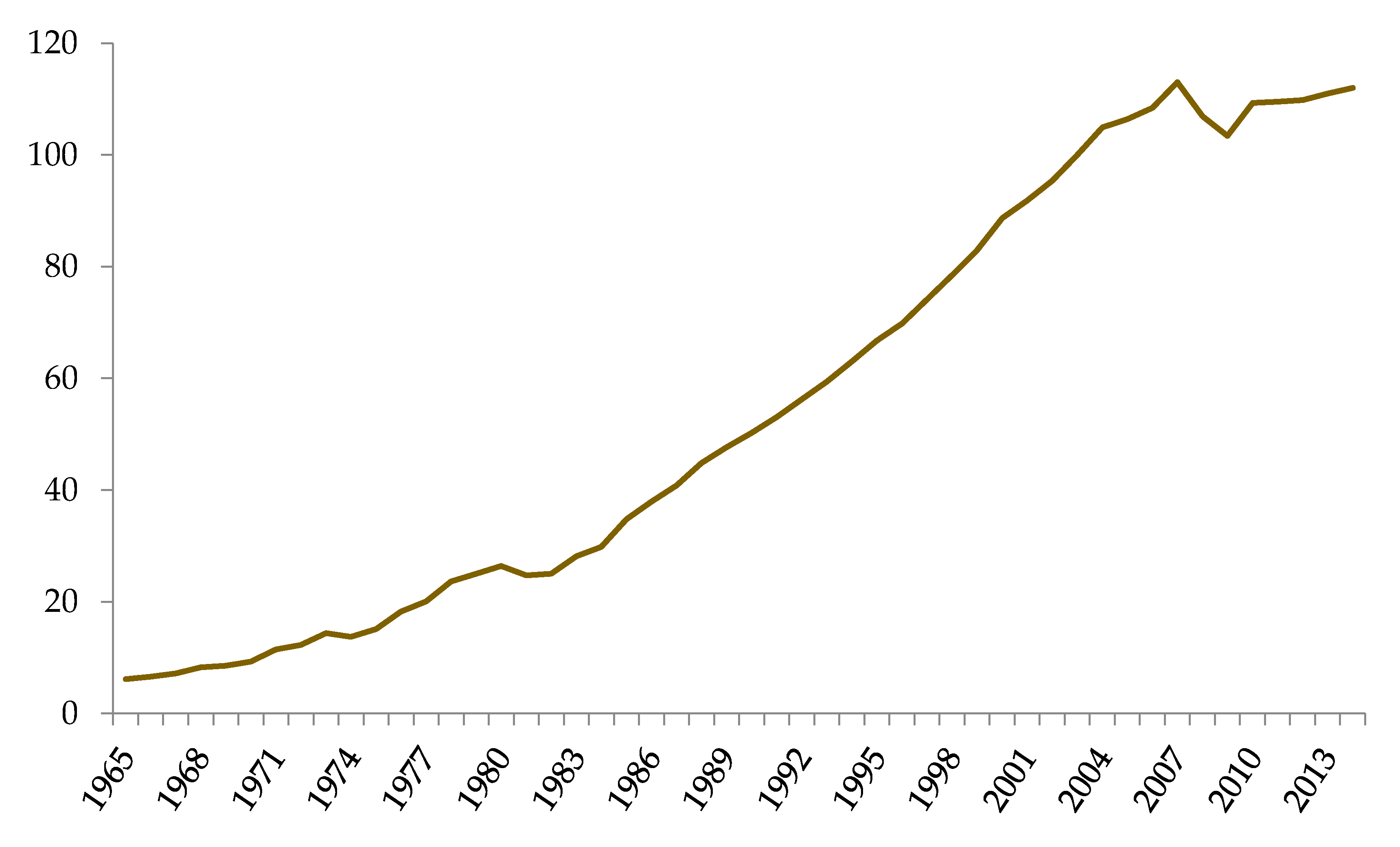
In this study, the time series of the Taiwanese primary energy consumption (Figure 2) was adopted to verify the effectiveness of the prediction models. Annual primary energy consumption from 1965 to 2014 was provided by BP [1]. The time series was separated into two subsets where 90% (46 samples) of the dataset were chosen as the training set while the remaining 10% (4 samples) were selected as the test set for verifying the prediction efficiency.

For accurate predictions, the original dataset will be transformed by the EEMD method. After the decomposition of the time series, the results of decompositions can be further predicted by the ARIMA method. Then, the prediction results derived from the ARIMA method will be aggregated as the final prediction results for energy consumption.

Meanwhile, such procedures can be extended by adopting SVR. Moreover, to help build the training model and avoid overfitting risks, the k-fold cross-validation was introduced into model construction within the prediction process. The k-fold cross-validation is used in SVR prediction error examinations based on selected hyperparameters from GA. In this study, the authors adopt five-fold cross-validation. A five-fold validation entails that all samples are divided into five portions; four of the five portions are used for training, and one of the five portions is for testing. The process is repeated five times. At first, the GA algorithm generates a set of hyperparameters. Through the five-fold cross-validation, we can obtain a performance. Next, the GA algorithm will continue to generate different hyperparameters based on cross-validation, thus obtaining a performance. Finally, we can select the best hyperparameters in terms of the best performances. The training data was randomly divided into $k$ subsamples. Among the $k$ samples, the $k-1$ subsamples were selected as the training data, and the remaining subsample was considered as validation data for testing the model. This research adopted 5-fold cross-validation into the model construction process.

4.3. Data Preprocessing Using EEMD Decomposition

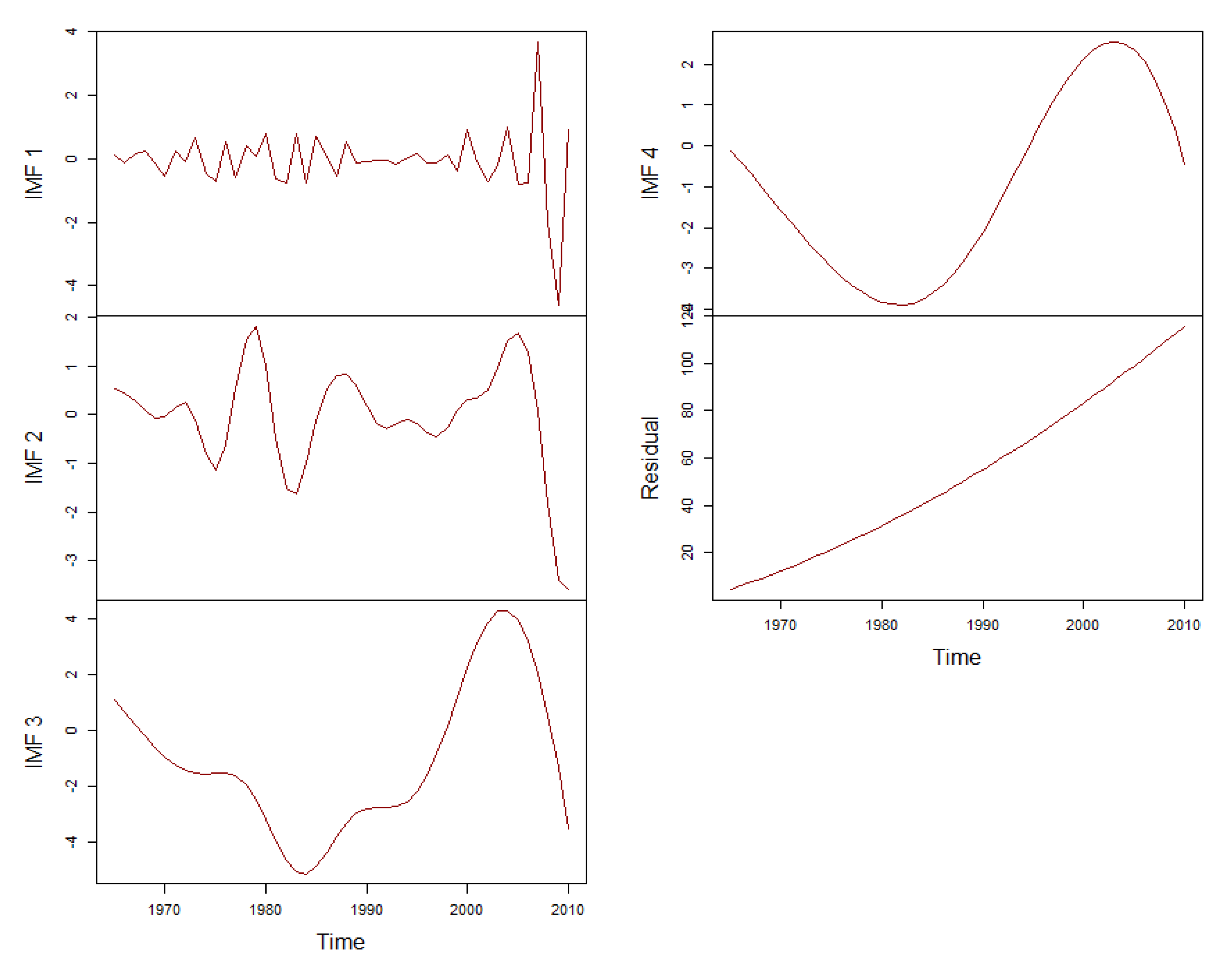
Before conducting the prediction using the proposed hybrid framework, the time series of energy consumptions will be processed using the EEMD decomposition method, which separates the original time series into several IMFs and a residue. The results are depicted in Figure 3. The four independent IMF components correspond to different frequency bands of the time series, which range from high to low.

In Figure 3, the IMFs stand for changing frequencies, amplitudes, and wavelengths. IMF₁ represents the highest frequency, maximum amplitude, and the shortest wavelength. The frequencies and amplitudes associated with the rest of the IMFs are lower while the wavelengths are longer. The residue represents a mode slowly varying around the long-term average.

4.4. Forecasting with the ARIMA Model

To establish the prediction model of primary energy consumption in terms of the historical time series dataset, the ARIMA method is introduced. Since the ARIMA model must be built into the series stationarity, the $d$ times difference needs to be obtained to have an ARIMA ($p,d,q$) model with $d$ as the order of differencing used. To test the stationarity of $d$ times differencing, the augmented Dickey–Fuller (ADF) test is utilized.

The construction of the ARIMA model depends on model identification. Here, differencing will be important for solving non-stationarity. Moreover, the order of AR ($p$) and MA ($q$) needs to be identified. Through ACF and PACF, the order of AR ($p$) and MA ($q$) can further be determined [28]. However, the ACF and PACF method may not be useful when performing hybrid ARMA processes. Commonly, AIC or BIC measures can be used to easily inspect the appropriateness of the ARMA model. In this research, the best forecasting model is determined based on AIC measures and statistically significant results. Once the forecasting model has been selected, the nonlinear method based on the optimization approach will be integrated into this model.

First, the stationary test for the decomposed data series and the first difference of the original time series derived from the ADF test is implemented and shown in

Table 1. Stationary analysis of primary energy consumption in Taiwan.

Difference and Decomposition	Specification	t-Value	Critical Value
			1%	5%	10%
First difference of original values	Trend	−4.267	−4.150	−3.500	−3.180
	Drift	−2.869	−3.580	−2.930	−2.600
	None	−1.792	−2.620	−1.950	−1.610
IMF1	Trend	−10.045	−4.150	−3.500	−3.180
	Drift	−10.000	−3.580	−2.930	−2.600
	None	−10.022	−2.620	−1.950	−1.610
IMF2	Trend	−9.793	−4.150	−3.500	−3.180
	Drift	−9.954	−3.580	−2.930	−2.600
	None	−10.066	−2.620	−1.950	−1.610
IMF3	Trend	−4.431	−4.150	−3.500	−3.180
	Drift	−4.797	−3.580	−2.930	−2.600
	None	−4.801	−2.620	−1.950	−1.610
IMF4	Trend	−46.468	−4.150	−3.500	−3.180
	Drift	−20.728	−3.580	−2.930	−2.600
	None	−7.099	−2.620	−1.950	−1.610

. According to the results of the ADF test, all the data series belonged to the stationary. That is, all the transformed data can be used to model constructions.

To further determine the parameters of the ARIMA order, ACF and PACF will be utilized. Likewise, such a procedure can also be followed for the decomposed data set using EEMD. To simplify the analytical procedure of EEMD-ARIMA, the corresponding ACF and PACF diagrams are not presented here.

Through the AIC and the statistical significance test, the suitable ARIMA models can be derived for the first difference time series and decomposed time series via the EEMD. Then the optimal form is specified as ARIMA(1,1,1). Table 1 shows the test results in the first difference of the original sequence. The original sequence is not stationary. Based on the first difference in the original difference, the sequence shows a stable status. Therefore, the difference $d$ will be set as 1. IMF1 ~ IMF4 and the residual are derived from the original sequence using the EEMD method. The sum of the IMFs and the residual is equal to the original sequence. 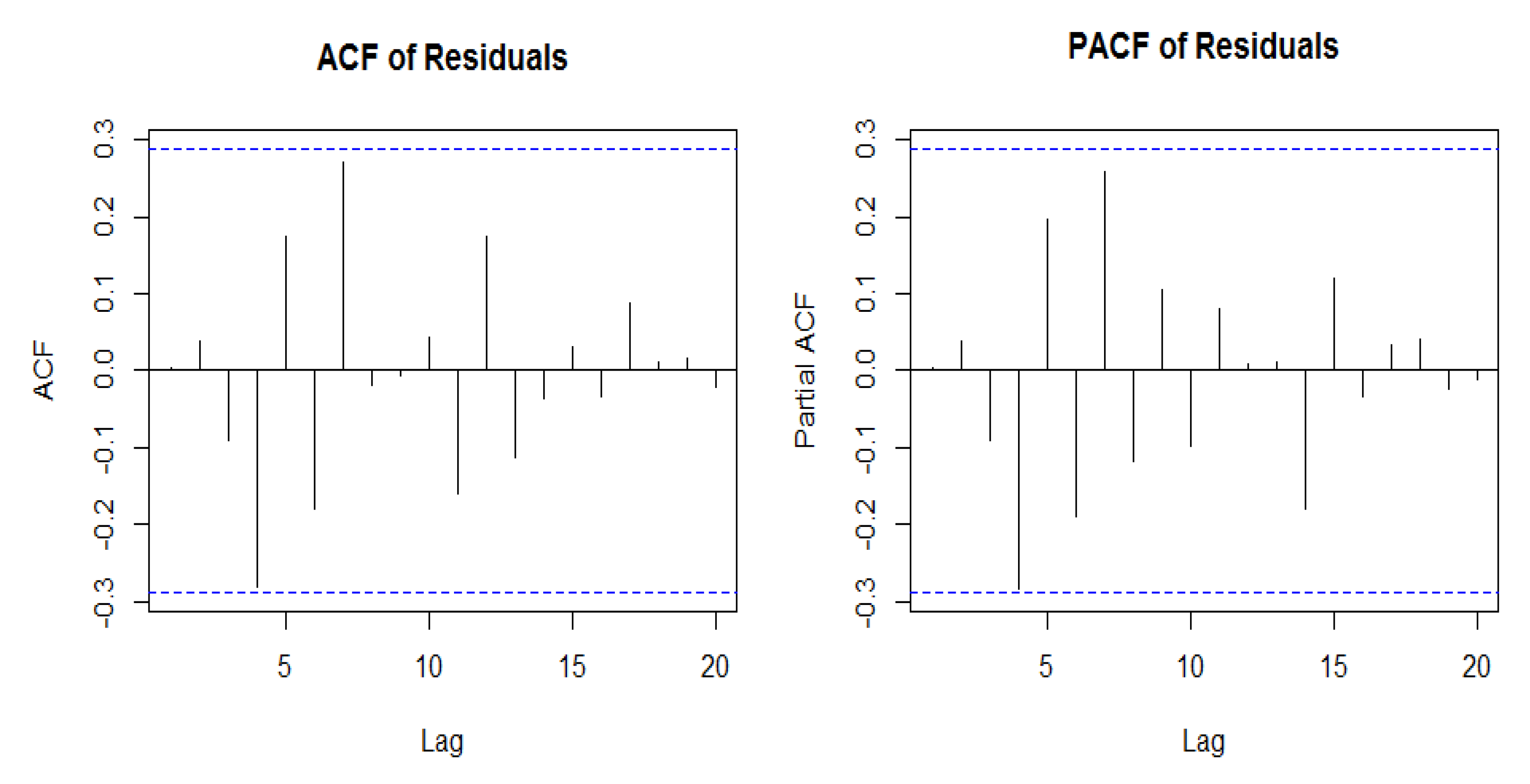The rationality has already been explained in the fourth paragraph of Section 3.1, where the original sequence was split into several different sequences. The sum of decomposed sequences equals to original sequence. Finally, after determining the proper parameters of the ARIMA models, whether the residual of the selected model possesses the autocorrelation problem should be confirmed. Therefore, the ACF and PACF tests were conducted to verify the selected model. Figure 4 demonstrates the estimated residuals using the ACF and PACF tests. According to the test results, no autocorrelation and partial autocorrelation exist within the residuals.

4.5. Forecasting with the EEMD-ARIMA-SVR Model Optimized by the GA Method

After building the EEMD-ARIMA model, the SVR method will be introduced to reduce the errors produced by ARIMA and enhance forecasting accuracy. According to earlier works, the prediction performance of the SVR method is outstanding; further, it can be fused with other nonlinear or linear methods successfully. Thus, after building the EEMD-ARIMA model, the SVR method will be introduced to reduce the errors produced by ARIMA and enhance forecasting accuracy.

Regarding the hybrid models in this research, the ARIMA initially served as a preprocessor to filter the linear pattern of the decomposed data series. Then, the error terms of the ARIMA model were fed into the SVR model to improve prediction accuracy. Generally, three parameters, $c, \epsilon , \mathrm{and} \gamma$, can influence the accuracy of the SVR model. Currently, no clear definition and standard procedure are available for determining the above three parameters [21]. However, the improper selection of the three parameters will cause either overfitting or underfitting. To prevent these, the GA method with cross-validation will be introduced to derive the best parameters for constructing the forecasting model. Meanwhile, some studies have pointed out that the utilization of the RBF can yield better prediction performance [21,22]. Thus, the RBF kernel with the 5-fold cross-validation based on the RMSE measure is adopted to help derive the best parameters of the SVR using GA. The above procedures will be applied to the ARIMA-SVR and EEMD-ARIMA-SVR models.

In GA, the number of iterations is set as 100, the population size is defined as 50, and the maximum number of iterations is defined as 50. The search boundaries for $c, \epsilon , \mathrm{and} \gamma$ are within the intervals $[\begin{array}{cc}{10}^{-4},& {10}^2\end{array}]$, $[\begin{array}{cc}{10}^{-4},& 2^{}\end{array}]$, and $[\begin{array}{cc}{2}^{-4},& 2^2\end{array}]$, respectively. The optimal values for $c, \epsilon , \mathrm{and} \gamma$ can thus be 0.441, 3.813, and 0.219, respectively. Further, the $c, \epsilon , \mathrm{and} \gamma$ parameters of the decomposed time series belonging to the four independent IMFs and the residual (Figure 3) are summarized in

Table 2. The parameter selection of forecasting model optimized by GA.

Models		c	γ	ε
ARIMA-GA-SVR		0.441	3.813	0.219
EEMD-ARIMA-GA-SVR	IMF1	0.995	1.072	0.195
	IMF2	4.775	0.852	0.100
	IMF3	0.751	1.134	0.461
	IMF4	0.304	3.308	0.470
	Residuals	0.022	1.501	0.352

. Once the parameters have been derived using GA, the optimal hybrid prediction model can be established.

4.6. Evaluations of Hybrid Models and Forecasting Results

After the construction of the hybrid models, the effectiveness of predictions will be compared further with those of different models including ARIMA, ARIMA-SVR, ARIMA-GA-SVR, EEMD-ARIMA, and EEMD-ARIMA-SVR. The superiority of the proposed EEMD-ARIMA-GA-SVR model of forecasting capability will be verified accordingly. The parameters derived using the GA with the fivefold cross-validation will be utilized to construct the SVR model. The parameters can yield better forecasting performances in related ARIMA-SVR models.

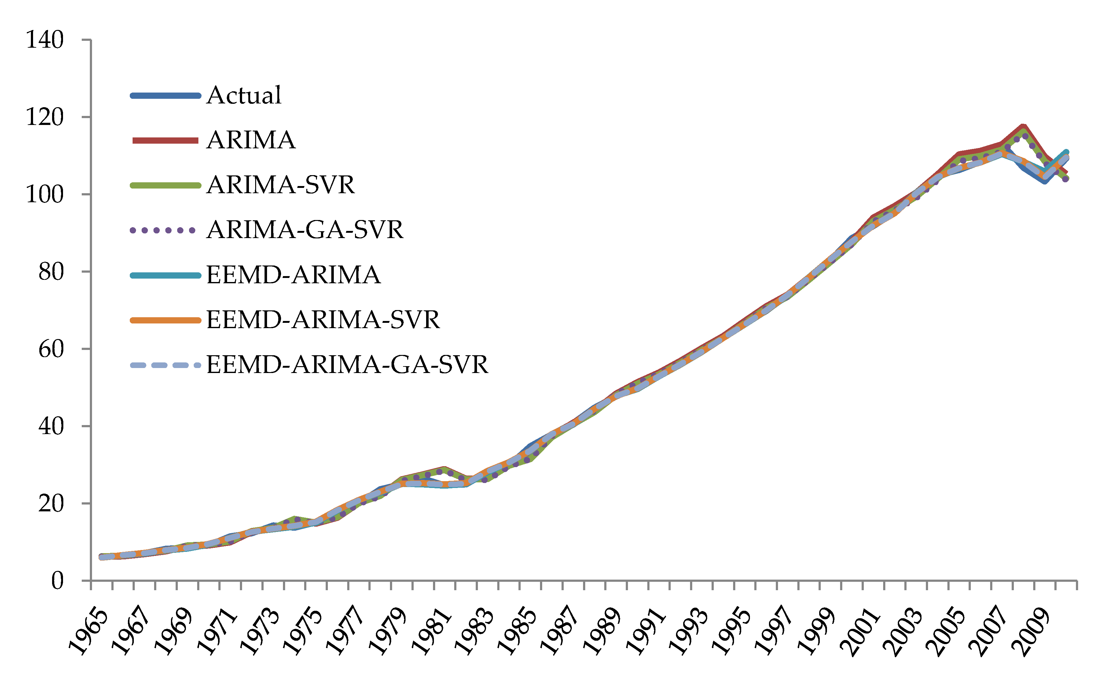
Based on the proposed hybrid framework and the five models for comparisons, the primary energy consumption in Taiwan for 2010–2014 is predicted and summarized in

Table 3. Data Test by four sample ranging from 2011 to 2014.

Year	2011	2012	2013	2014
Actual	109.542	109.797	110.959	112.019
ARIMA	111.896	114.527	117.200	119.914
ARIMA-SVR	110.579	113.137	115.735	118.372
ARIMA-GA-SVR	110.071	112.591	115.160	117.777
EEMD-ARIMA	113.174	110.733	111.934	115.542
EEMD-ARIMA-SVR	112.222	110.112	110.809	115.061
EEMD-ARIMA-GA-SVR	112.057	110.075	110.678	114.912

. According to the prediction results, EEMD-ARIMA-SVR and EEMD-ARIMA-GA-SVR outperformed the other four models. Meanwhile, the prediction results derived using ARIMA and ARIMA-SVR were unsatisfactory from the aspect of inconsistencies between predicted versus actual values. The four prediction performance measures, MAE, MAPE, MSE, and RMSE, derived from the six training models versus the actual values are illustrated in Figure 5 and summarized in

Table 4. Comparison of forecasting indices.

Models	Training				Testing
	MAE	MAPE (*)	MSE	RMSE	MAE	MAPE (*)	MSE	RMSE
ARIMA	1.397	3.704	5.669	2.381	5.305	4.782	32.301	5.683
ARIMA-SVR	1.285	3.467	4.535	2.130	3.877	3.491	18.851	4.342
ARIMA-GA-SVR	1.257	3.408	4.246	2.061	3.320	2.988	14.723	3.837
EEMD-ARIMA	0.499	1.429	0.611	0.781	2.266	2.048	6.856	2.618
EEMD-ARIMA-SVR	0.425	1.351	0.388	0.623	1.547	1.396	4.139	2.034
EEMD-ARIMA-GA-SVR	0.413	1.308	0.381	0.617	1.492	1.346	3.711	1.926

Remark: *: numbers in percentage.

. Based on the results of comparisons, the proposed model outperformed ARIMA. MAE and MSE decreased by 70.43% and 93.28% in the training stage, respectively; further, the two measures decreased by 71.89% and 88.51% in the testing stage, respectively. From the aspects of MAPE and RMSE, both measures improved by 64.68% and 74.07% in the training stage, respectively; they also improved by 71.85% and 66.10% in the testing stage, respectively.

The proposed model outperformed ARIMA-SVR. MAE and MSE decreased by 67.85% and 91.59% in the training stage, respectively; further, the two measures decreased by 61.52% and 80.31% in the testing stage, respectively. Meanwhile, MAPE and RMSE improved by 62.26% and 71.01% in the training stage and by 61.44% and 55.63% in the testing stage, respectively.

Compared with ARIMA-GA-SVR, the proposed model performed better as well. MAE and MSE decreased by 67.14% and 91.02%, in the training stage and by 55.08% and 74.79% in the testing stage, respectively. Further, MAPE and RMSE improved by 61.61% and 70.04% in the training stage and by 54.96% and 49.79% in the testing stage, respectively. Based on the above comparison results, the hybrid model integrated with the EEMD method showed better forecasting performance than other models without the data decomposition process.

The proposed model also outperformed EEMD-ARIMA. MAE and MSE decreased by 17.17% and 37.57% in the training stage and by 34.19% and 45.87% in the testing stage, respectively. Meanwhile, MAPE and RMSE were enhanced by 8.41% and 20.98% in the training stage and by 34.27% and 26.43% in the testing stage, respectively.

Compared with EEMD-ARIMA-SVR, the proposed framework performed better. From the aspect of MAE and MSE, the proposed framework outperformed EEMD-ARIMA-SVR by reducing both measures by 2.76% and 1.80% in the training stage and by 3.57% and 10.33% in the testing stage, respectively. At the same time, MAPE and RMSE were enhanced by 3.19% and 0.91% in the training stage and by 3.58% and 5.30% in the testing stage, respectively.

More specifically, from the aspect of training models, the hybrid models including EEMD-ARIMA-SVR and EEMD-ARIMA-GA-SVR performed better, with relatively smaller residual errors in comparison with results derived from any stand-alone or hybrid models. The predictions based on the models without the EEMD decomposition show the limited forecasting capability of the training models. Similarly, from the perspective of the testing model, the proposed model achieved better performance in predicting primary energy consumption. In this study, the comparison results show that the hybrid models with EEMD decomposition can significantly reduce overall forecasting errors. That is, the EEMD method is useful in manipulating the nonstationary time series; thus, better prediction results can be derived by integrating other forecasting methods. Further, GA can reduce forecasting errors by ARIMA-SVR. Based on the analytical results, the proposed EEMD-ARIMA-GA-SVR is a powerful tool and model for energy consumption prediction.

Finally, to identify the significant differences between the prediction results of any two models adopted in this work, the Wilcoxon signed-rank test is performed. This test was adopted extensively in examining the prediction results of two different models and justifying whether these results are significantly different based on small samples [37,38]. The null and alternative hypotheses are described as follows:

$$H_0: {\mu }_1-{\mu }_2=0 (\mathrm{null} \mathrm{hypothesis}) \mathrm{and}$$

$$H_1: {\mu }_1-{\mu }_2\ne 0 (\mathrm{alternative} \mathrm{hypothesis}),$$

where ${\mu }_1$ represents the mean of the actual data and ${\mu }_2$ stands for the mean of the predicted data. The Wilcoxon test can easily determine whether the mean differences are significant or not. All the $p$-values derived from the testing of the six pairs of methods were higher than 0.05. That is, no mean differences are observed between the test and predicted values derived from each method.

5. Conclusions

This study presented a hybrid prediction model consisting of ARIMA, SVR, EEMD, and GA. The empirical results have verified the feasibility of the proposed method. Such a hybrid model that combines linear and nonlinear patterns based on the ARIMA and the SVR models as well as adopts data preprocessing and parameter optimization for time series predictions can produce more precise prediction results. From the aspect of limitations and future research possibilities, different datasets on energy consumption can be used at the same time to evaluate whether the forecasting performance of the proposed model will be the best among all prediction models. The data post-processing procedure can be integrated; the differences of the prediction results derived from the proposed model and the framework consisting of the post-processing procedure can be compared. In the future, a dynamic procedure in terms of multiple-step-ahead forecasting can be adopted to replace the one-step-ahead forecasting techniques being used in this work. Much more meaningful and valuable information can be derived for decision-makers in energy predictions.